↗ arXiv ↗ Hugging Face ↗ Papers with Code
TL;DR#
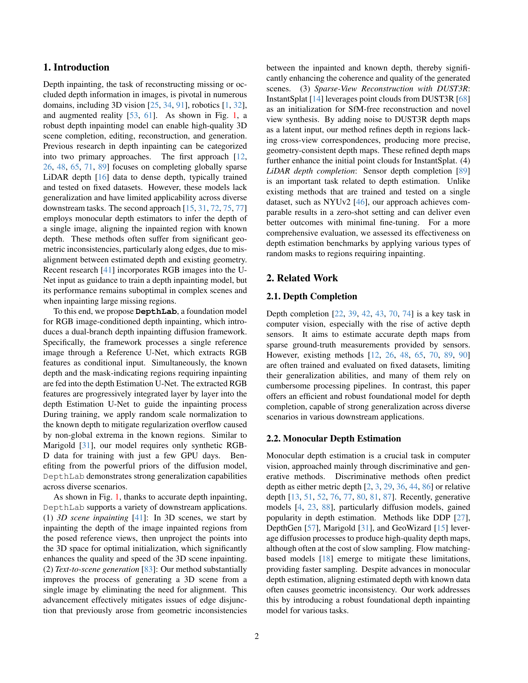
Many computer vision tasks involve incomplete depth information. Existing depth inpainting methods struggle with complex scenes, limited generalization, and geometric inconsistencies. This paper introduces DepthLab, a novel foundation model that addresses these issues. DepthLab uses a dual-branch diffusion framework that incorporates both RGB image features and known depth information. It processes data via a Reference U-Net for RGB features and a Depth Estimation U-Net that integrates RGB features for guided inpainting, and employs a novel masking strategy and random scale normalization.
DepthLab outperforms existing methods on multiple benchmarks for various applications including 3D scene inpainting, text-to-scene generation, and LiDAR depth completion. Its strength lies in reliable completion of both continuous and isolated missing depth regions while preserving scale consistency. The availability of source code makes DepthLab a valuable tool for broader research and development in depth-related tasks.
Key Takeaways#
Why does it matter?#
This paper is important because it introduces DepthLab, a novel and robust foundation model for depth inpainting that significantly improves upon existing methods. Its ability to generalize across diverse downstream tasks, its resilience to depth-deficient regions, and its ability to preserve scale consistency makes it a valuable tool for researchers in 3D vision and related fields. Furthermore, the availability of source code is vital for facilitating further research and development in depth completion methods.
Visual Insights#

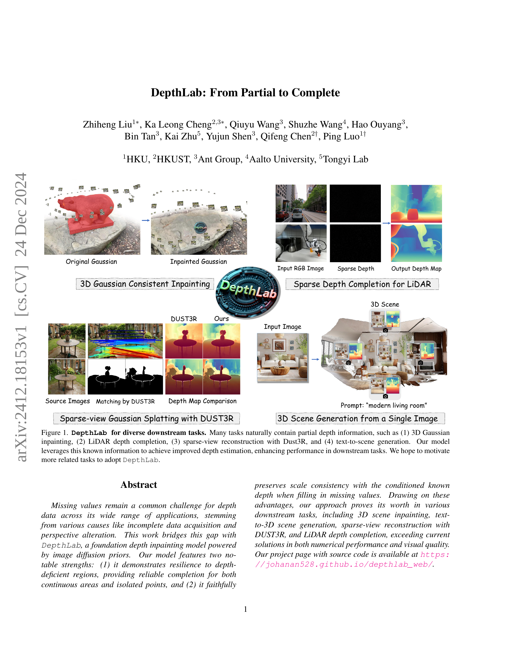
🔼 DepthLab is a foundational model for depth inpainting that leverages known partial depth information from various sources to improve depth estimation across diverse downstream applications. The figure showcases four such applications: (1) filling in missing parts of a 3D Gaussian surface; (2) completing incomplete depth data from LiDAR sensors; (3) reconstructing a full 3D scene from sparse views using the DUST3R method; and (4) generating a 3D scene from a text prompt. By incorporating this pre-existing depth information, DepthLab achieves better performance in these tasks than models that lack this capability.
read the caption
Figure 1: DepthLab for diverse downstream tasks. Many tasks naturally contain partial depth information, such as (1) 3D Gaussian inpainting, (2) LiDAR depth completion, (3) sparse-view reconstruction with Dust3R, and (4) text-to-scene generation. Our model leverages this known information to achieve improved depth estimation, enhancing performance in downstream tasks. We hope to motivate more related tasks to adopt DepthLab.
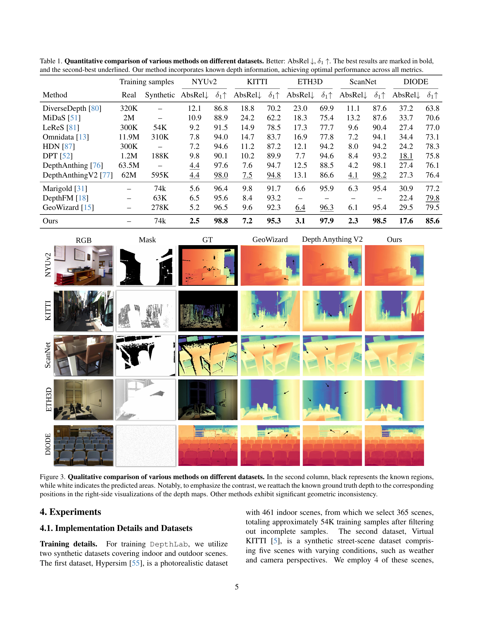
| Method | Real | Synthetic | NYUv2 AbsRel↓ δ₁↑ | NYUv2 δ₁↑ | KITTI AbsRel↓ δ₁↑ | KITTI δ₁↑ | ETH3D AbsRel↓ δ₁↑ | ETH3D δ₁↑ | ScanNet AbsRel↓ δ₁↑ | ScanNet δ₁↑ | DIODE AbsRel↓ δ₁↑ | DIODE δ₁↑ |
|---|---|---|---|---|---|---|---|---|---|---|---|---|
| DiverseDepth [80] | 320K | – | 12.1 | 86.8 | 18.8 | 70.2 | 23.0 | 69.9 | 11.1 | 87.6 | 37.2 | 63.8 |
| MiDaS [51] | 2M | – | 10.9 | 88.9 | 24.2 | 62.2 | 18.3 | 75.4 | 13.2 | 87.6 | 33.7 | 70.6 |
| LeReS [81] | 300K | 54K | 9.2 | 91.5 | 14.9 | 78.5 | 17.3 | 77.7 | 9.6 | 90.4 | 27.4 | 77.0 |
| Omnidata [13] | 11.9M | 310K | 7.8 | 94.0 | 14.7 | 83.7 | 16.9 | 77.8 | 7.2 | 94.1 | 34.4 | 73.1 |
| HDN [87] | 300K | – | 7.2 | 94.6 | 11.2 | 87.2 | 12.1 | 94.2 | 8.0 | 94.2 | 24.2 | 78.3 |
| DPT [52] | 1.2M | 188K | 9.8 | 90.1 | 10.2 | 89.9 | 7.7 | 94.6 | 8.4 | 93.2 | 18.1 | 75.8 |
| DepthAnthing [76] | 63.5M | – | 4.4 | 97.6 | 7.6 | 94.7 | 12.5 | 88.5 | 4.2 | 98.1 | 27.4 | 76.1 |
| DepthAnthingV2 [77] | 62M | 595K | 4.4 | 98.0 | 7.5 | 94.8 | 13.1 | 86.6 | 4.1 | 98.2 | 27.3 | 76.4 |
| Marigold [31] | – | 74k | 5.6 | 96.4 | 9.8 | 91.7 | 6.6 | 95.9 | 6.3 | 95.4 | 30.9 | 77.2 |
| DepthFM [18] | – | 63K | 6.5 | 95.6 | 8.4 | 93.2 | – | – | – | – | 22.4 | 79.8 |
| GeoWizard [15] | – | 278K | 5.2 | 96.5 | 9.6 | 92.3 | 6.4 | 96.3 | 6.1 | 95.4 | 29.5 | 79.5 |
| Ours | – | 74k | 2.5 | 98.8 | 7.2 | 95.3 | 3.1 | 97.9 | 2.3 | 98.5 | 17.6 | 85.6 |
🔼 This table presents a quantitative comparison of different depth estimation methods across various datasets (NYUv2, KITTI, ETH3D, ScanNet, and DIODE). The metrics used for comparison are Absolute Relative Error (AbsRel) and the percentage of pixels with an absolute relative error less than 1.25 (δ1). Lower AbsRel values and higher δ1 values indicate better performance. The table highlights the best and second-best results for each metric and dataset, clearly showing that the proposed ‘Ours’ method outperforms all others. A key aspect is that the ‘Ours’ method incorporates known depth information, which is a crucial factor contributing to its superior performance.
read the caption
Table 1: Quantitative comparison of various methods on different datasets. Better: AbsRel ↓↓\downarrow↓, δ1subscript𝛿1\delta_{1}italic_δ start_POSTSUBSCRIPT 1 end_POSTSUBSCRIPT ↑↑\uparrow↑. The best results are marked in bold, and the second-best underlined. Our method incorporates known depth information, achieving optimal performance across all metrics.
In-depth insights#
Depth Inpainting#
Depth inpainting, the focus of this research, addresses the challenge of reconstructing missing or incomplete depth information in images. This is crucial because many real-world depth datasets are inherently incomplete, due to factors such as sensor limitations, occlusions, or data acquisition difficulties. The paper explores the use of a novel dual-branch diffusion framework, which efficiently leverages both RGB image information and known partial depth data to achieve accurate and consistent completion. A key advantage is its robustness to various types of missing depth patterns, unlike traditional approaches that often struggle with irregular or large-scale missing regions. By combining image features and depth information, the framework ensures that the inpainted depth aligns seamlessly with existing geometry, eliminating geometric inconsistencies. The use of diffusion models provides powerful priors, improving generalization capabilities and enabling application across multiple downstream tasks, such as 3D scene inpainting, text-to-3D generation, and sparse view reconstruction. The reliance on synthetic data during training further enhances the model’s generalizability and reduces the dependence on large, meticulously annotated datasets. Ultimately, Depth inpainting as presented here represents a valuable advancement in addressing the pervasive issue of missing depth information, broadening the applicability of depth-based applications.
Diffusion Priors#
The concept of “Diffusion Priors” in the context of depth inpainting is a powerful idea. It leverages the inherent strengths of diffusion models, specifically their ability to generate realistic and coherent samples from noise. By using a pre-trained diffusion model, the network implicitly incorporates rich prior knowledge about image and depth data distributions. This avoids the need for extensive training on specific depth datasets, reducing training time and improving generalization. The diffusion prior acts as a powerful regularizer, guiding the inpainting process towards plausible depth completions. This is particularly important in handling complex scenes and large missing depth regions. A key benefit is the preservation of scale consistency, ensuring the inpainted depth seamlessly blends with the existing known depth, avoiding artifacts and geometric inconsistencies. Integrating diffusion priors elegantly combines the benefits of diffusion models’ powerful generative capabilities with the task-specific constraints of depth inpainting, leading to high-quality and robust results. This strategy opens up new possibilities for other computer vision tasks where incorporating prior knowledge efficiently is crucial.
Downstream Tasks#
The research paper explores various downstream applications of the proposed DepthLab model, highlighting its versatility and robustness. Depth inpainting, a core component of DepthLab, serves as the foundation for several advanced tasks. The ability to accurately reconstruct missing or incomplete depth information enhances the efficacy of other tasks relying on depth data. 3D scene inpainting benefits greatly from DepthLab’s ability to fill gaps in depth maps, creating more complete and realistic 3D scenes. Similarly, text-to-scene generation leverages DepthLab to improve the generation of 3D scenes from text prompts by providing more accurate and complete depth information. Sparse-view reconstruction with DUST3R (an existing method) is improved significantly through DepthLab’s refinement of depth maps, addressing limitations in generating accurate reconstructions in areas lacking viewpoint overlap. Finally, LiDAR depth completion, a critical task for autonomous driving, is further improved through DepthLab’s robustness and ability to generalize across various datasets, outperforming traditional methods in both accuracy and generalization. The numerous successful downstream applications of DepthLab demonstrate its significant contributions to various fields reliant on depth data.
Zero-Shot Generalization#
Zero-shot generalization, the ability of a model to perform well on unseen tasks or datasets without any explicit training on those specific tasks, is a highly desirable characteristic in machine learning. In the context of depth inpainting, this means a model should be capable of accurately completing missing depth information in images it has never encountered before, adapting to various data distributions, sensor types, and levels of occlusion. DepthLab’s success in zero-shot settings across multiple datasets highlights a significant advance. The use of pre-trained diffusion models and a robust dual-branch framework likely contributes to this generalization ability. The pre-trained weights provide a strong prior knowledge about image and depth data, while the framework effectively integrates RGB information and known depth cues for reliable inpainting. Future work should focus on further enhancing the model’s robustness to handle extreme cases of sparsity or complex scenes, and investigation into theoretical understanding of why zero-shot performance is achieved would be beneficial. Furthermore, exploration of applications in scenarios with significantly different imaging modalities could validate the true limits of this generalization capability, leading to a better understanding of its effectiveness in real-world scenarios.
Future Directions#
The ‘Future Directions’ section of this research paper on DepthLab could explore several promising avenues. Improving sampling speed is crucial; current diffusion models can be computationally expensive. Investigating alternative sampling methods, such as consistency models or flow-based approaches, could significantly enhance efficiency. Another key area is enhancing the handling of sparse depth data. The current VAE struggles with extremely sparse inputs; exploring alternative encoding techniques or pre-processing methods tailored for sparse data is important. Finally, extending DepthLab’s capabilities beyond depth completion would expand its impact. Integrating normal estimation into the framework would allow for more sophisticated 3D scene editing and manipulation, and exploring applications in areas like 4D scene reconstruction would open new opportunities. Ultimately, the future of DepthLab hinges on addressing these computational and functional limitations, making it more versatile and accessible to a wider range of applications.
More visual insights#
More on figures

🔼 DepthLab’s training process involves two key components: the Reference U-Net, which extracts RGB features from the input image; and the Estimation U-Net, which processes the depth information. The training process starts by randomly masking parts of the ground truth depth map and then interpolating the masked areas. Both the original and interpolated depth maps undergo random scale normalization before being fed into their respective encoders. The Reference and Estimation U-Nets are then combined using a layer-by-layer feature fusion technique. This approach enables DepthLab to leverage both visual and depth cues to generate precise depth maps, especially in complex areas with significant missing data.
read the caption
Figure 2: The training process of DepthLab. First, we apply random masking to the ground truth depth to create the masked depth, followed by interpolation. Both the interpolated masked depth and the original depth undergo random scale normalization before being fed into the encoder. The Reference U-Net extracts RGB features, while the Estimation U-Net takes the noisy depth, masked depth, and encoded mask as input. Layer-by-layer feature fusion allows for finer-grained visual guidance, achieving high-quality depth predictions even in large or complex masked regions.

🔼 This figure compares the performance of different depth completion methods on several datasets. The leftmost column shows the input RGB images. The second column displays the input depth maps, where black indicates known depth values and white represents missing data. The next three columns present the depth maps generated by three different state-of-the-art methods (GeoWizard, DepthAnything V2, and the proposed method). Notably, the known ground truth depth data is re-integrated into the output visualizations of the competing methods to highlight geometric inconsistencies and contrast them against the method proposed in the paper.
read the caption
Figure 3: Qualitative comparison of various methods on different datasets. In the second column, black represents the known regions, while white indicates the predicted areas. Notably, to emphasize the contrast, we reattach the known ground truth depth to the corresponding positions in the right-side visualizations of the depth maps. Other methods exhibit significant geometric inconsistency.

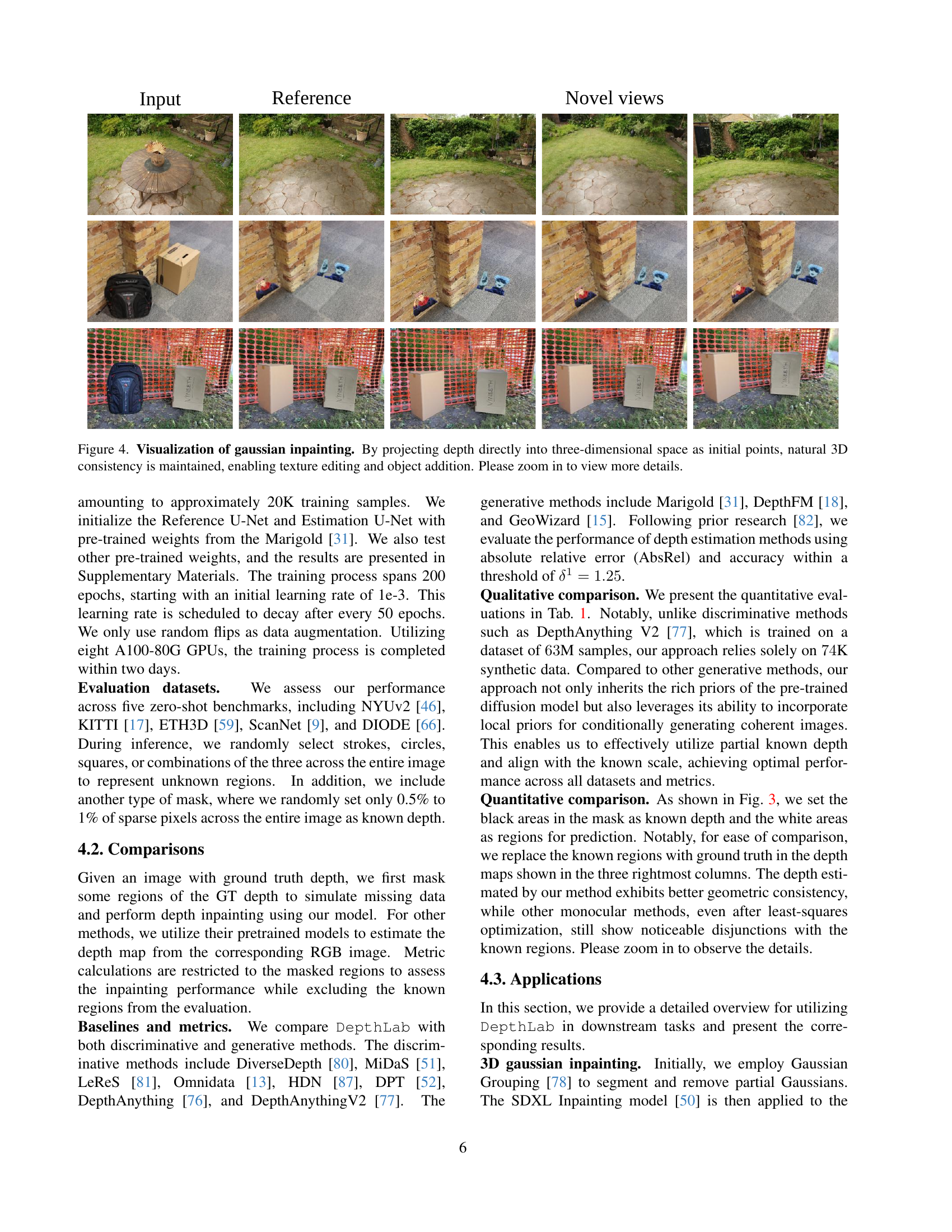
🔼 Figure 4 showcases the results of Gaussian inpainting achieved by DepthLab. The process starts by directly projecting the depth map into 3D space, using the known depth values as a foundation. This 3D representation ensures the natural consistency of the scene. The model’s ability to maintain this consistency allows for seamless texture editing and the addition of new objects to the scene without introducing artifacts or inconsistencies. Zooming in reveals finer details of the high-quality inpainting results.
read the caption
Figure 4: Visualization of gaussian inpainting. By projecting depth directly into three-dimensional space as initial points, natural 3D consistency is maintained, enabling texture editing and object addition. Please zoom in to view more details.

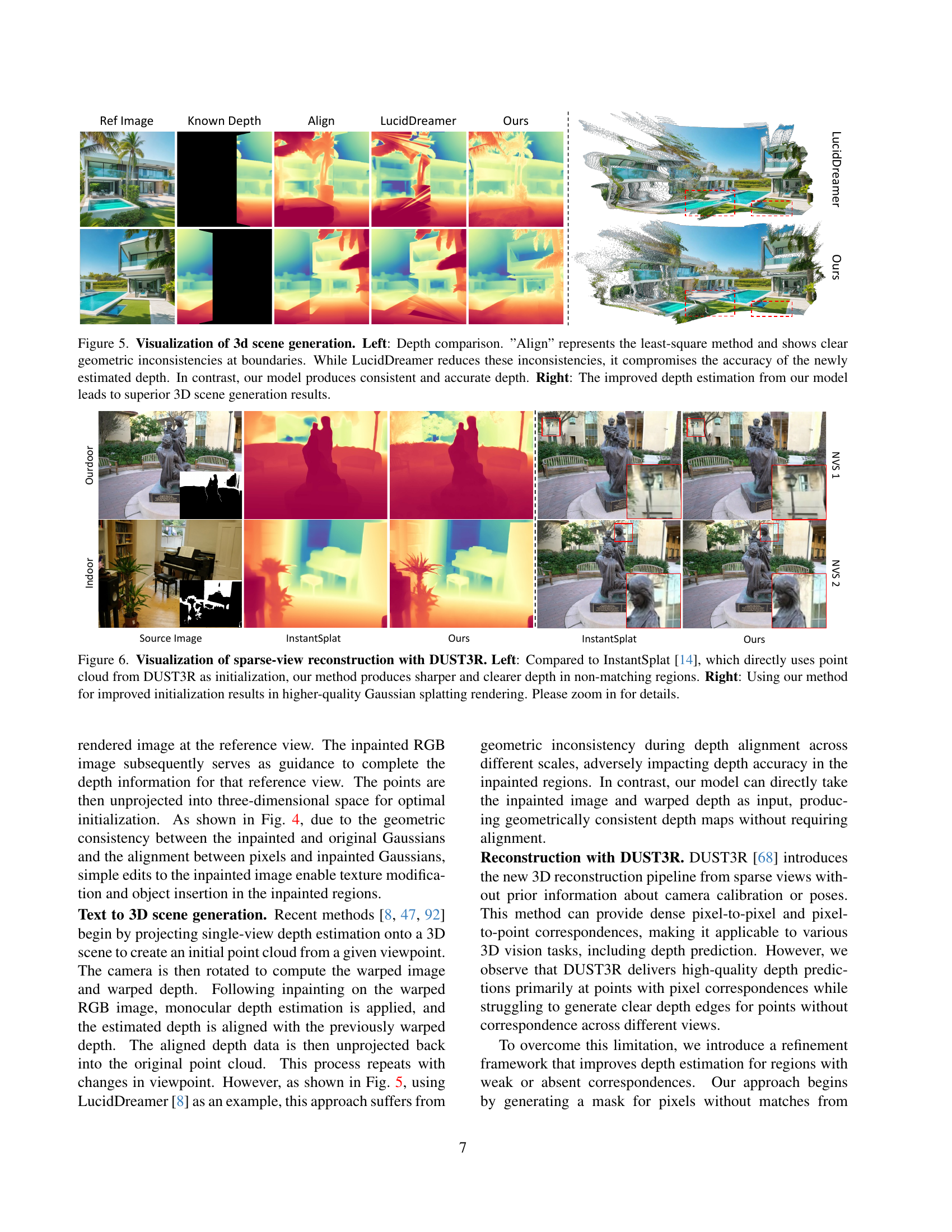
🔼 Figure 5 presents a comparison of 3D scene generation results using different depth estimation methods. The left side shows a depth comparison, highlighting the geometric inconsistencies produced by the least-squares method (‘Align’) and how LucidDreamer, while improving upon the least-squares approach, still compromises accuracy in newly estimated depth regions. In contrast, the proposed DepthLab model produces consistent and accurate depth estimation. The right side demonstrates the superior 3D scene generation quality achieved using depth estimations from the DepthLab model. This illustrates DepthLab’s ability to produce high-quality 3D reconstructions by accurately inpainting depth data.
read the caption
Figure 5: Visualization of 3d scene generation. Left: Depth comparison. ”Align” represents the least-square method and shows clear geometric inconsistencies at boundaries. While LucidDreamer reduces these inconsistencies, it compromises the accuracy of the newly estimated depth. In contrast, our model produces consistent and accurate depth. Right: The improved depth estimation from our model leads to superior 3D scene generation results.
More on tables
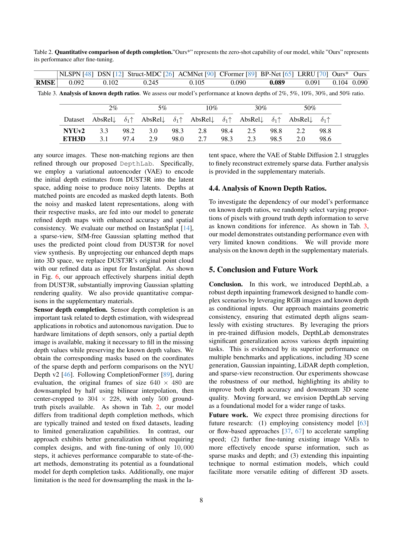
| Method | RMSE |
|---|---|
| NLSPN [48] | 0.092 |
| DSN [12] | 0.102 |
| Struct-MDC [26] | 0.245 |
| ACMNet [90] | 0.105 |
| CFormer [89] | 0.090 |
| BP-Net [65] | 0.089 |
| LRRU [70] | 0.091 |
| Ours* | 0.104 |
| Ours | 0.090 |
🔼 Table 2 presents a quantitative comparison of different depth completion methods. The results show the performance of several existing methods and the proposed DepthLab model. The table specifically highlights two variations of DepthLab: ‘Ours*’, representing the model’s performance without fine-tuning (zero-shot), and ‘Ours’, showcasing the performance after fine-tuning. This allows for a direct comparison of the model’s inherent capabilities versus its potential after additional training.
read the caption
Table 2: Quantitative comparison of depth completion.”Ours*” represents the zero-shot capability of our model, while ”Ours” represents its performance after fine-tuning.
| Dataset | 2% AbsRel↓ | 2% δ₁↑ | 5% AbsRel↓ | 5% δ₁↑ | 10% AbsRel↓ | 10% δ₁↑ | 30% AbsRel↓ | 30% δ₁↑ | 50% AbsRel↓ | 50% δ₁↑ |
|---|---|---|---|---|---|---|---|---|---|---|
| NYUv2 | 3.3 | 98.2 | 3.0 | 98.3 | 2.8 | 98.4 | 2.5 | 98.8 | 2.2 | 98.8 |
| ETH3D | 3.1 | 97.4 | 2.9 | 98.0 | 2.7 | 98.3 | 2.3 | 98.5 | 2.0 | 98.6 |
🔼 This table presents a quantitative analysis of the model’s performance under varying ratios of known depth information. Specifically, it evaluates the model’s accuracy using AbsRel and 81 metrics across five different known depth ratios: 2%, 5%, 10%, 30%, and 50%. This allows for an assessment of the model’s robustness and generalization capabilities when dealing with incomplete depth data. The results are presented for the NYUv2 and ETH3D datasets.
read the caption
Table 3: Analysis of known depth ratios. We assess our model’s performance at known depths of 2%, 5%, 10%, 30%, and 50% ratio.
Full paper#
