↗ arXiv ↗ Hugging Face ↗ Papers with Code
TL;DR#
Large Language Models (LLMs) are powerful but computationally expensive. Many struggle with complex reasoning tasks, hindering real-world applications. Existing models often require significant resources for training and fine-tuning, making them inaccessible to many researchers.
This paper introduces Xmodel-2, a 1.2-billion parameter LLM designed for reasoning. It uses a novel architecture that allows for efficient scaling and transfer of configurations, maximizing training efficiency and stability. Xmodel-2 achieves state-of-the-art performance in complex reasoning and agent-based tasks, while being open-source and low-cost. Its success highlights the potential for efficient model design to address the limitations of large language models.
Key Takeaways#
Why does it matter?#
This paper is important because it introduces Xmodel-2, a novel 1.2B parameter language model that excels in reasoning tasks. Its open-source nature and efficient design make it an accessible and valuable resource for researchers. The findings on efficient model design and training strategies advance the state-of-the-art and open new avenues for research in reasoning capabilities. The paper also demonstrates the potential of efficient model design and training strategies to address the challenges of computationally expensive large language models.
Visual Insights#

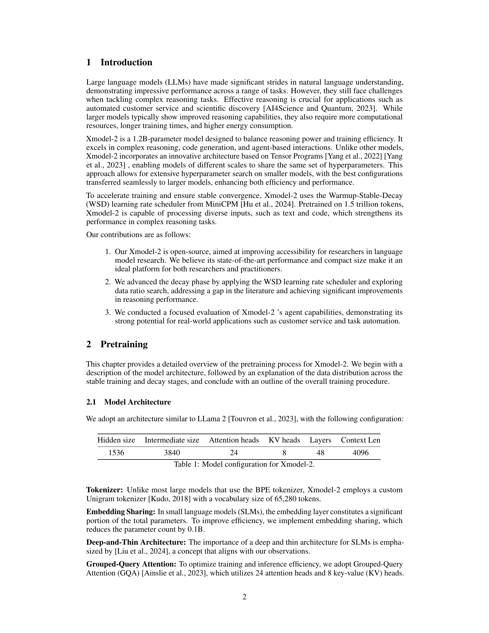
🔼 This figure displays the average scores achieved by various large language models (LLMs) on six complex reasoning benchmarks: GSM8K, MATH, BBH, MMLU, HumanEval, and MBPP. The x-axis represents the model size in billions of parameters, and the y-axis represents the average score across the six benchmarks. Each point represents a different LLM, with Xmodel-2 highlighted. The figure visually compares the performance of Xmodel-2 to other LLMs of similar size, demonstrating its competitive performance on complex reasoning tasks.
read the caption
Figure 1: Average Scores on Complex Reasoning Benchmarks (GSM8K, MATH, BBH, MMLU, HumanEval and MBPP).
| Hidden size | Intermediate size | Attention heads | KV heads | Layers | Context Len |
|---|---|---|---|---|---|
| 1536 | 3840 | 24 | 8 | 48 | 4096 |
🔼 This table details the architectural hyperparameters of the Xmodel-2 language model. It lists the hidden size, intermediate size, number of attention heads, number of key-value heads, number of layers, and the context length. These values define the model’s capacity and computational requirements.
read the caption
Table 1: Model configuration for Xmodel-2.
In-depth insights#
Efficient LLM Design#
Efficient LLM design is crucial for widespread adoption, focusing on balancing model performance with computational resource constraints. Reducing parameter count without sacrificing accuracy is key; techniques like embedding sharing and deep-and-thin architectures are promising approaches. Training efficiency is paramount, necessitating optimized learning rate schedulers (like the WSD scheduler) and careful exploration of data ratios to improve convergence speed and stability. The choice of tokenizer and attention mechanism also greatly impacts efficiency, with techniques like Unigram tokenizers and Grouped-Query Attention emerging as efficient alternatives. Finally, hardware-aware design and model quantization strategies will be important considerations for deploying LLMs on resource-limited devices, enabling wider accessibility and usage.
WSD Learning Rate#
The Warmup-Stable-Decay (WSD) learning rate scheduler is a crucial element in Xmodel-2’s training process. Its effectiveness stems from its three-phase approach: an initial warmup phase, followed by a stable phase maintaining a consistent learning rate, and finally a decay phase where the rate gradually decreases. This strategy addresses common challenges in training large language models (LLMs), such as instability and vanishing gradients. The warmup phase helps the model to avoid early overfitting, allowing it to learn robust initial representations. The stable phase enables efficient learning at an optimal pace before transitioning to the decay phase. The gradual decay prevents a sudden disruption to the learning process, ensuring a smooth convergence and better generalization. By using WSD, Xmodel-2 achieves superior training efficiency and stability compared to methods using traditional learning rate schedules. The integration of WSD is a significant design choice that directly contributes to Xmodel-2’s state-of-the-art performance, showcasing a clear understanding of the nuances of LLM training.
Reasoning Benchmarks#
A dedicated section on “Reasoning Benchmarks” within a research paper would be crucial for evaluating the performance of a language model, especially one focused on reasoning tasks. It should detail the specific benchmarks used, providing clear descriptions of each dataset’s characteristics. This would include the type of reasoning tasks involved (e.g., commonsense, logical, mathematical), the dataset sizes, and any specific formats or question types. Crucially, the rationale behind selecting these particular benchmarks needs explanation, justifying their relevance to the model’s capabilities and addressing potential biases. The results section should present a comprehensive analysis of the model’s performance on each benchmark, ideally including quantitative metrics like accuracy, F1 score, or exact match, along with qualitative analyses for a deeper understanding. Comparing the model’s performance against established baselines and state-of-the-art models would provide valuable context and demonstrate its strengths and weaknesses relative to existing technology. A discussion of limitations of the benchmarks themselves should also be included, acknowledging any potential shortcomings in capturing the full spectrum of reasoning abilities.
Agent Capabilities#
The section on ‘Agent Capabilities’ would explore the LLM’s ability to perform complex tasks requiring multi-step reasoning and decision-making within simulated environments. This would involve evaluating performance on diverse agent-based tasks, such as question answering using multiple sources (HotpotQA), fact verification (FEVER), navigation in a simulated environment (AlfWorld), and e-commerce interactions (WebShop). The evaluation metrics would likely include success rates and exact match accuracy, providing a comprehensive assessment of the LLM’s real-world applicability. A key insight would be how the LLM’s reasoning abilities translate into effective action selection and planning within these complex scenarios. The results would highlight strengths and weaknesses, revealing areas where the model excels and areas requiring further development. This section’s findings are critical for understanding the practical implications of the LLM’s capabilities and its potential for various real-world applications, beyond simple question-answering benchmarks.
Scaling Law Analysis#
A scaling law analysis in a large language model (LLM) research paper would typically investigate the relationship between model size, training data, and performance. A key focus would be establishing empirical relationships to predict performance on unseen data given changes in these parameters. The analysis might involve plotting performance metrics (accuracy, loss, perplexity) against model size, exploring power-law relationships often observed in LLMs. Understanding the scaling behavior is crucial for resource allocation, allowing researchers to determine the optimal balance between model size and performance gains for a given budget. The analysis would likely consider different training regimes and data distributions, investigating how varying these factors impacts the scaling laws. Furthermore, a discussion of diminishing returns and limitations would be essential, providing insights into the point where increasing model size or data yields only marginal performance improvements, allowing researchers to identify cost effective model design and training strategies.
More visual insights#
More on figures

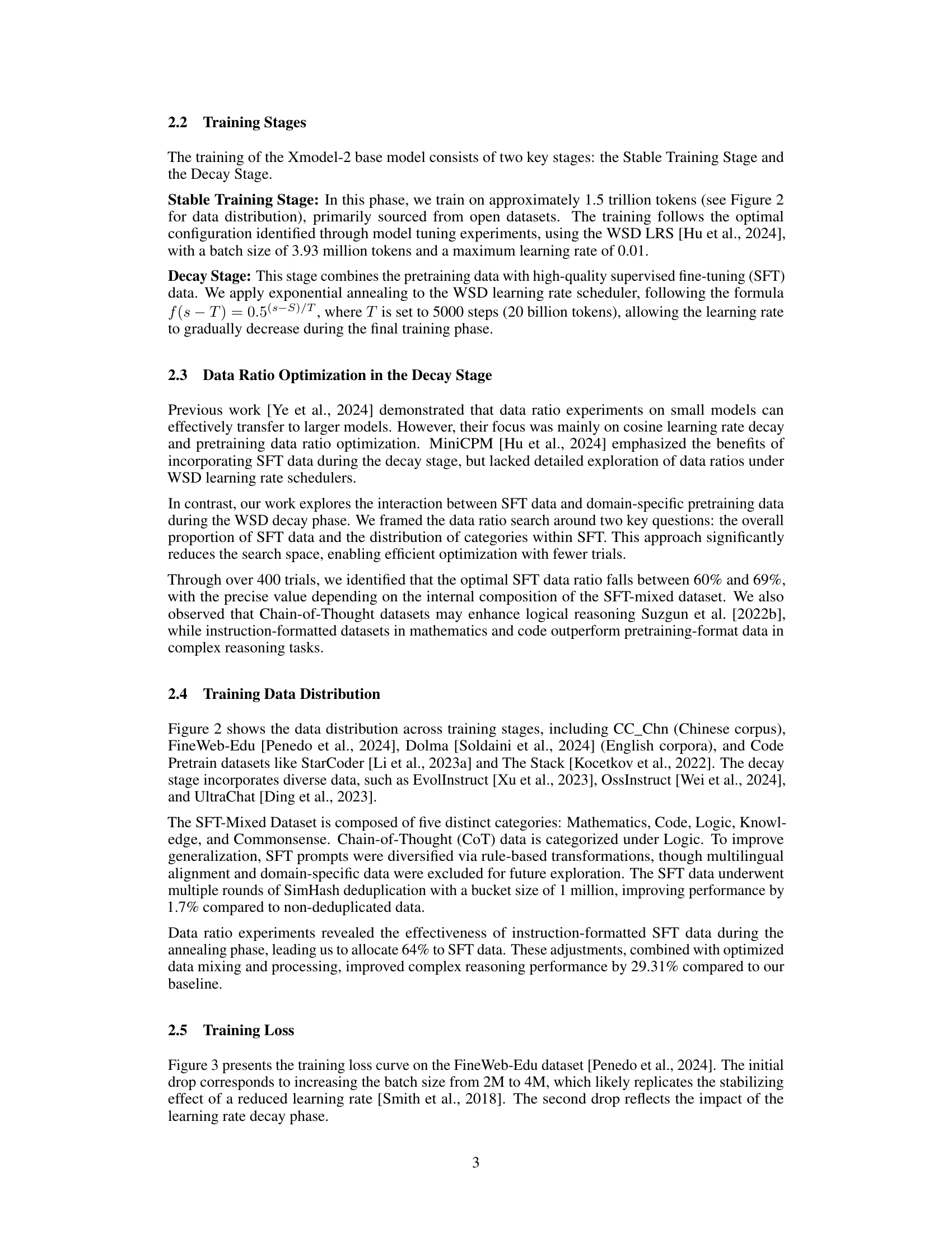
🔼 This figure shows the composition of the datasets used during the training of the Xmodel-2 language model. The training process is divided into two stages: a stable training phase and a decay phase. The left pie chart details the data sources and their proportions used in the stable training phase. The right pie chart illustrates the distribution of data sources in the decay phase, which includes additional supervised fine-tuning (SFT) data. The difference in dataset compositions highlights the shift in training strategies between the two phases.
read the caption
Figure 2: Data mixture of different training stages.The left side represents the stable training phase, and the right side represents the decay phase.

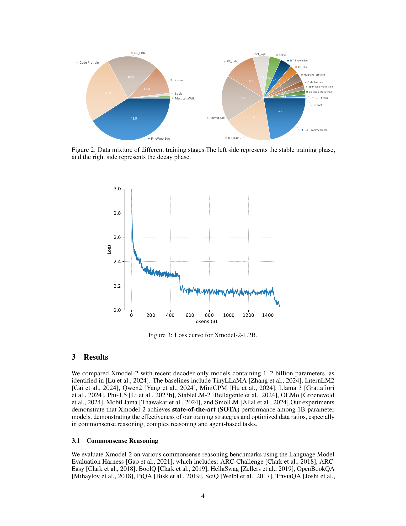
🔼 This figure shows the training loss curve for the Xmodel-2 1.2 billion parameter model. The x-axis represents the number of tokens processed in billions, and the y-axis represents the loss value. The curve shows a general downward trend, indicating that the model is learning and improving over time. There are two notable drops in the loss, which may correspond to changes in the training process, such as the introduction of supervised fine-tuning data or adjustments to the learning rate scheduler. The figure provides a visual representation of the model’s training progress and its convergence to a lower loss, suggesting that the model is being trained effectively.
read the caption
Figure 3: Loss curve for Xmodel-2-1.2B.

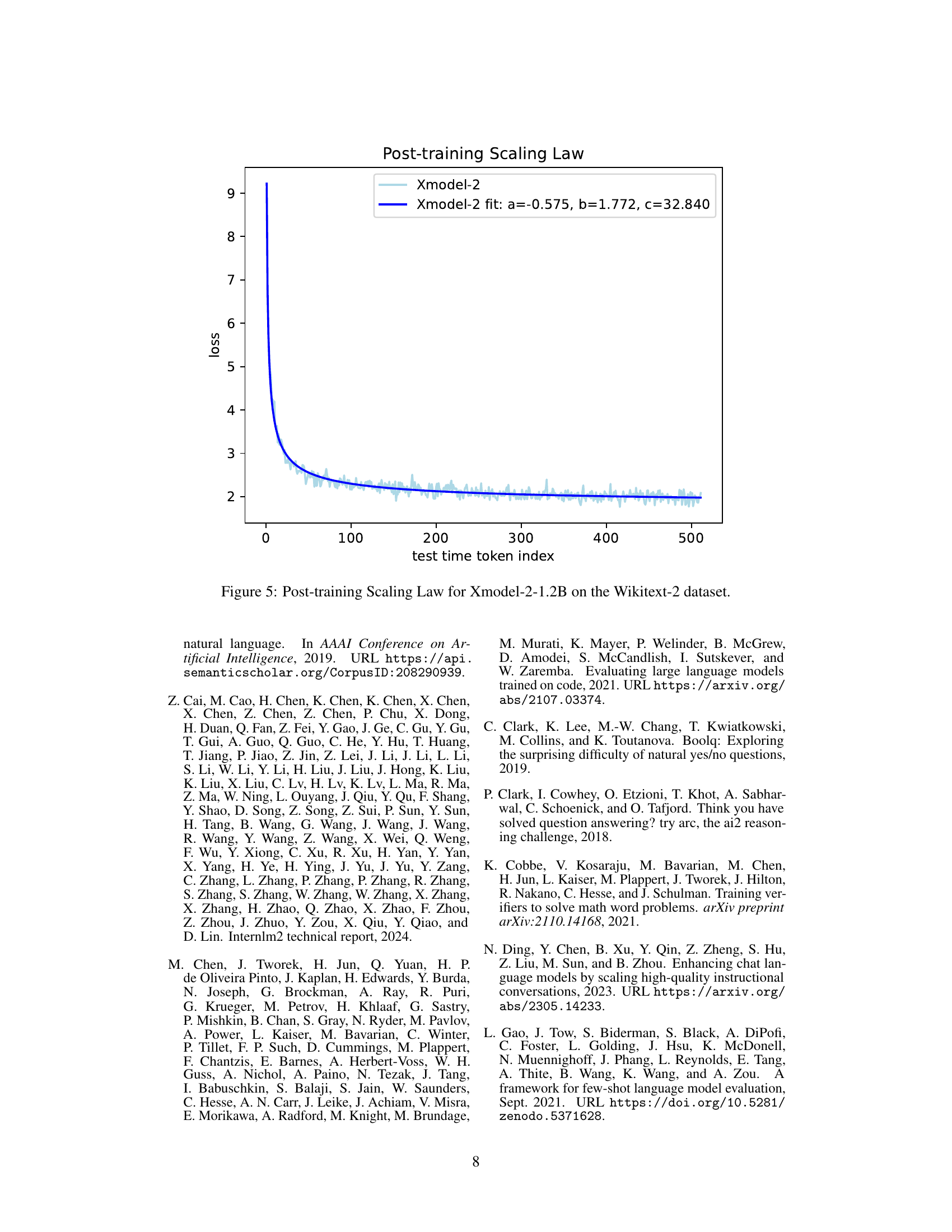
🔼 This calibration plot visualizes the reliability of the pre-trained Xmodel-2-1.2B model’s confidence scores when predicting answers on the MMLU (Massive Multitask Language Understanding) dataset. The x-axis represents the model’s predicted probability (confidence) of a given answer being correct, ranging from 0 to 1. The y-axis shows the actual accuracy or proportion of correctly predicted answers among those with the corresponding confidence score. A perfectly calibrated model would show a diagonal line, indicating that a prediction with, for example, 70% confidence is correct 70% of the time. Deviations from this line highlight areas where the model is either overconfident (predicting high probability but having low accuracy) or underconfident (predicting low probability but achieving high accuracy). The plot helps assess the trustworthiness and reliability of the model’s predictions.
read the caption
Figure 4: Calibration plot for the pre-trained Xmodel-2-1.2B model on the MMLU dataset.

🔼 This figure illustrates the relationship between the number of tokens used during testing and the resulting loss (perplexity) for the Xmodel-2-1.2B model on the Wikitext-2 dataset. The x-axis represents the number of test-time tokens, while the y-axis displays the loss. The curve demonstrates a power-law relationship, indicating that increasing the context length initially leads to significant reductions in loss, though this improvement diminishes with further increases in context length. A fitted curve is included to capture this diminishing returns effect, showing the power-law relationship between loss and token index.
read the caption
Figure 5: Post-training Scaling Law for Xmodel-2-1.2B on the Wikitext-2 dataset.
More on tables
| Model | ARC-c | ARC-e | Boolq | HS. | OB. | PiQA | SciQ | Wino. | Avg |
|---|---|---|---|---|---|---|---|---|---|
| MobiLlama-1B | 28.24 | 61.53 | 60.92 | 46.74 | 21.80 | 75.14 | 88.20 | 59.27 | 55.23 |
| TinyLLaMA1.1-1.1B | 30.97 | 61.66 | 55.99 | 46.70 | 25.20 | 72.63 | 89.30 | 59.43 | 55.24 |
| OLMo-1B | 28.67 | 63.34 | 61.74 | 46.97 | 25.00 | 75.03 | 87.00 | 59.98 | 55.97 |
| OpenELM-1.1B | 28.84 | 62.37 | 63.58 | 48.36 | 25.40 | 74.76 | 90.60 | 61.72 | 56.95 |
| Llama-3.2-1B | 31.31 | 65.36 | 63.73 | 47.78 | 26.40 | 74.48 | 91.50 | 61.01 | 57.70 |
| MiniCPM-1.2B | 36.86 | 70.29 | 67.92 | 49.91 | 23.60 | 74.43 | 91.80 | 60.77 | 59.45 |
| Fox-1-1.6B | 34.73 | 69.91 | 71.77 | 46.33 | 24.60 | 75.24 | 93.20 | 60.77 | 59.57 |
| InternLM2.5-1.8B | 35.24 | 66.37 | 79.82 | 46.99 | 22.00 | 73.29 | 94.90 | 62.67 | 60.16 |
| Qwen2-1.5B | 33.11 | 66.41 | 72.60 | 48.57 | 27.00 | 75.57 | 94.60 | 65.75 | 60.45 |
| StableLM-2-zephyr-1.6B | 36.52 | 66.79 | 80.00 | 53.26 | 26.80 | 74.86 | 88.00 | 64.09 | 61.29 |
| SmolLM-1.7B | 43.43 | 76.47 | 65.93 | 49.58 | 30.00 | 75.79 | 93.20 | 60.93 | 61.92 |
| Qwen2.5-1.5B | 41.21 | 75.21 | 72.97 | 50.15 | 31.80 | 75.90 | 94.30 | 63.61 | 63.14 |
| DCLM-1B | 41.30 | 74.79 | 71.41 | 53.59 | 32.20 | 76.93 | 94.00 | 66.22 | 63.81 |
| Phi-1.5-1.3B | 44.80 | 76.22 | 74.95 | 47.96 | 38.60 | 76.66 | 93.30 | 72.93 | 65.68 |
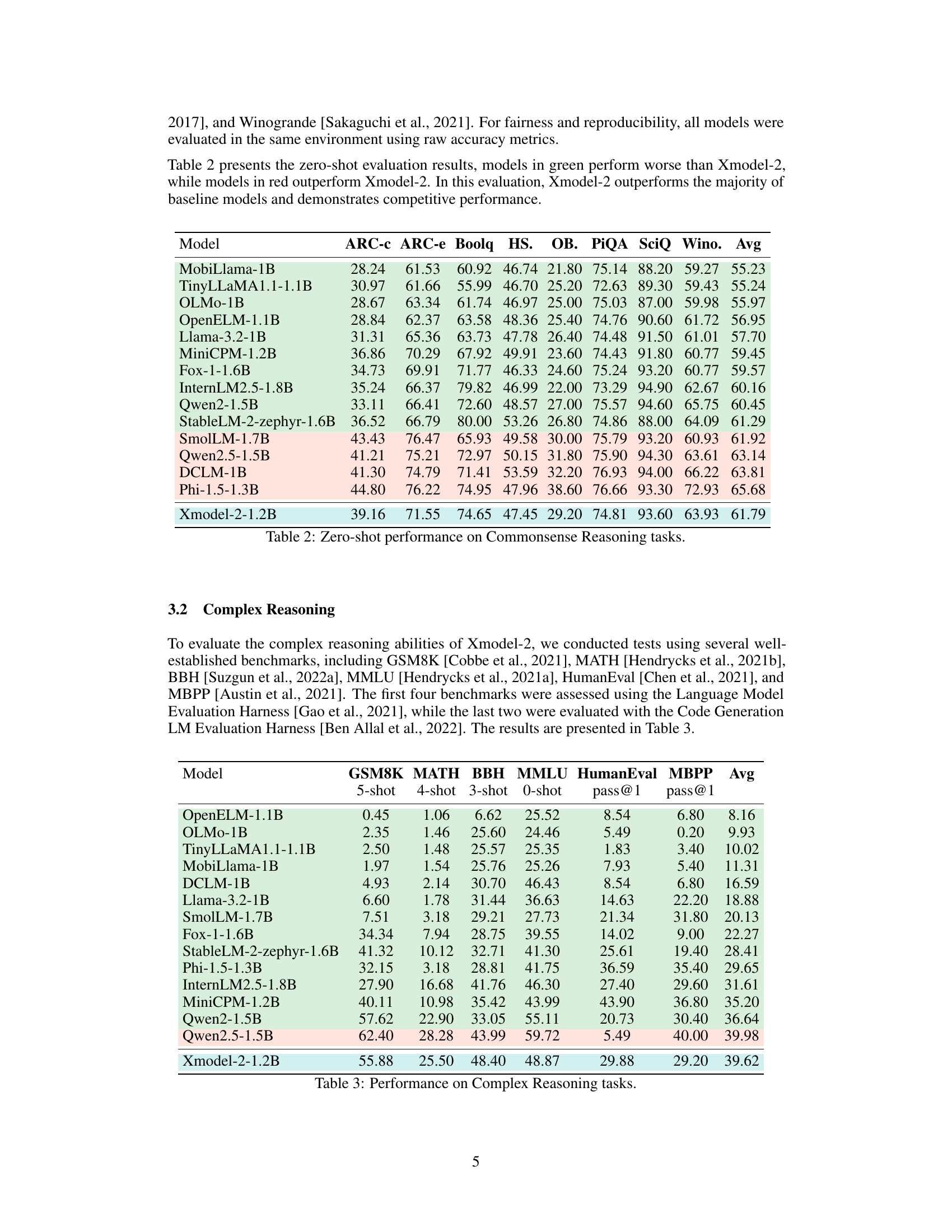
| Xmodel-2-1.2B | 39.16 | 71.55 | 74.65 | 47.45 | 29.20 | 74.81 | 93.60 | 63.93 | 61.79 |
🔼 This table presents the results of a zero-shot evaluation on several commonsense reasoning benchmarks. Zero-shot means the model was not fine-tuned on these specific datasets; it used only its pre-trained knowledge. The benchmarks assess various aspects of commonsense understanding. The table compares the performance of Xmodel-2 against other similar-sized language models (around 1-2 billion parameters), showcasing its performance relative to these baselines. The scores reflect the accuracy of the models on each task, offering a comprehensive view of their commonsense reasoning abilities.
read the caption
Table 2: Zero-shot performance on Commonsense Reasoning tasks.
| Model | GSM8K 5-shot | MATH 4-shot | BBH 3-shot | MMLU 0-shot | HumanEval pass@1 | MBPP pass@1 | Avg |
|---|---|---|---|---|---|---|---|
| OpenELM-1.1B | 0.45 | 1.06 | 6.62 | 25.52 | 8.54 | 6.80 | 8.16 |
| OLMo-1B | 2.35 | 1.46 | 25.60 | 24.46 | 5.49 | 0.20 | 9.93 |
| TinyLLaMA1.1-1.1B | 2.50 | 1.48 | 25.57 | 25.35 | 1.83 | 3.40 | 10.02 |
| MobiLlama-1B | 1.97 | 1.54 | 25.76 | 25.26 | 7.93 | 5.40 | 11.31 |
| DCLM-1B | 4.93 | 2.14 | 30.70 | 46.43 | 8.54 | 6.80 | 16.59 |
| Llama-3.2-1B | 6.60 | 1.78 | 31.44 | 36.63 | 14.63 | 22.20 | 18.88 |
| SmolLM-1.7B | 7.51 | 3.18 | 29.21 | 27.73 | 21.34 | 31.80 | 20.13 |
| Fox-1-1.6B | 34.34 | 7.94 | 28.75 | 39.55 | 14.02 | 9.00 | 22.27 |
| StableLM-2-zephyr-1.6B | 41.32 | 10.12 | 32.71 | 41.30 | 25.61 | 19.40 | 28.41 |
| Phi-1.5-1.3B | 32.15 | 3.18 | 28.81 | 41.75 | 36.59 | 35.40 | 29.65 |
| InternLM2.5-1.8B | 27.90 | 16.68 | 41.76 | 46.30 | 27.40 | 29.60 | 31.61 |
| MiniCPM-1.2B | 40.11 | 10.98 | 35.42 | 43.99 | 43.90 | 36.80 | 35.20 |
| Qwen2-1.5B | 57.62 | 22.90 | 33.05 | 55.11 | 20.73 | 30.40 | 36.64 |
| Qwen2.5-1.5B | 62.40 | 28.28 | 43.99 | 59.72 | 5.49 | 40.00 | 39.98 |
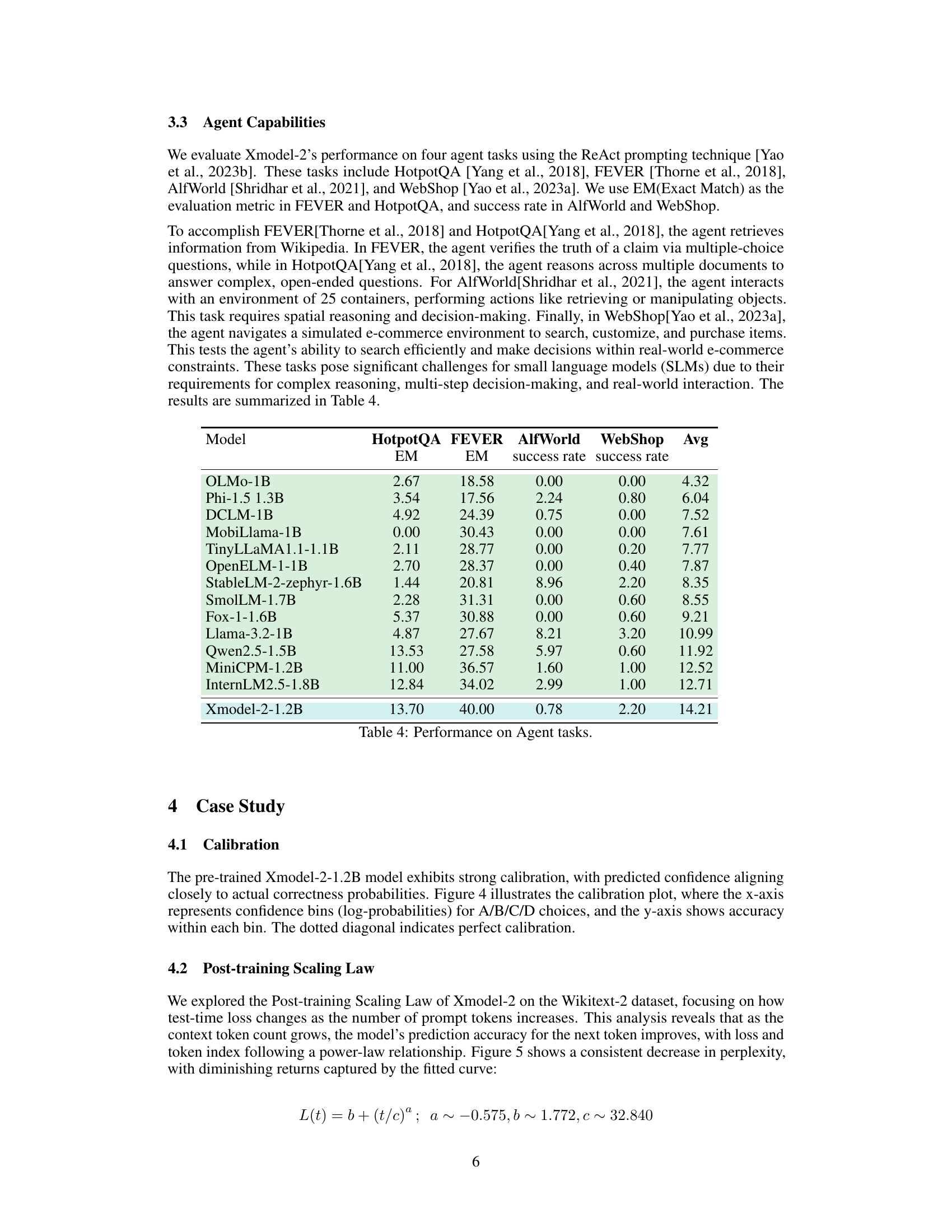
| Xmodel-2-1.2B | 55.88 | 25.50 | 48.40 | 48.87 | 29.88 | 29.20 | 39.62 |
🔼 This table presents the performance of Xmodel-2 and various other large language models on six complex reasoning benchmarks: GSM8K, MATH, BBH, MMLU, HumanEval, and MBPP. For each model, the table shows its performance (average score) on each benchmark, and the average performance across all benchmarks. The benchmarks assess different aspects of reasoning ability, including mathematical problem-solving, commonsense reasoning, and code generation. The results allow for a comparison of Xmodel-2’s performance against other models of similar size and architecture in complex reasoning tasks.
read the caption
Table 3: Performance on Complex Reasoning tasks.
| Model | HotpotQA EM | FEVER EM | AlfWorld success rate | WebShop success rate | Avg |
|---|---|---|---|---|---|
| OLMo-1B | 2.67 | 18.58 | 0.00 | 0.00 | 4.32 |
| Phi-1.5 1.3B | 3.54 | 17.56 | 2.24 | 0.80 | 6.04 |
| DCLM-1B | 4.92 | 24.39 | 0.75 | 0.00 | 7.52 |
| MobiLlama-1B | 0.00 | 30.43 | 0.00 | 0.00 | 7.61 |
| TinyLLaMA1.1-1.1B | 2.11 | 28.77 | 0.00 | 0.20 | 7.77 |
| OpenELM-1-1B | 2.70 | 28.37 | 0.00 | 0.40 | 7.87 |
| StableLM-2-zephyr-1.6B | 1.44 | 20.81 | 8.96 | 2.20 | 8.35 |
| SmolLM-1.7B | 2.28 | 31.31 | 0.00 | 0.60 | 8.55 |
| Fox-1-1.6B | 5.37 | 30.88 | 0.00 | 0.60 | 9.21 |
| Llama-3.2-1B | 4.87 | 27.67 | 8.21 | 3.20 | 10.99 |
| Qwen2.5-1.5B | 13.53 | 27.58 | 5.97 | 0.60 | 11.92 |
| MiniCPM-1.2B | 11.00 | 36.57 | 1.60 | 1.00 | 12.52 |
| InternLM2.5-1.8B | 12.84 | 34.02 | 2.99 | 1.00 | 12.71 |
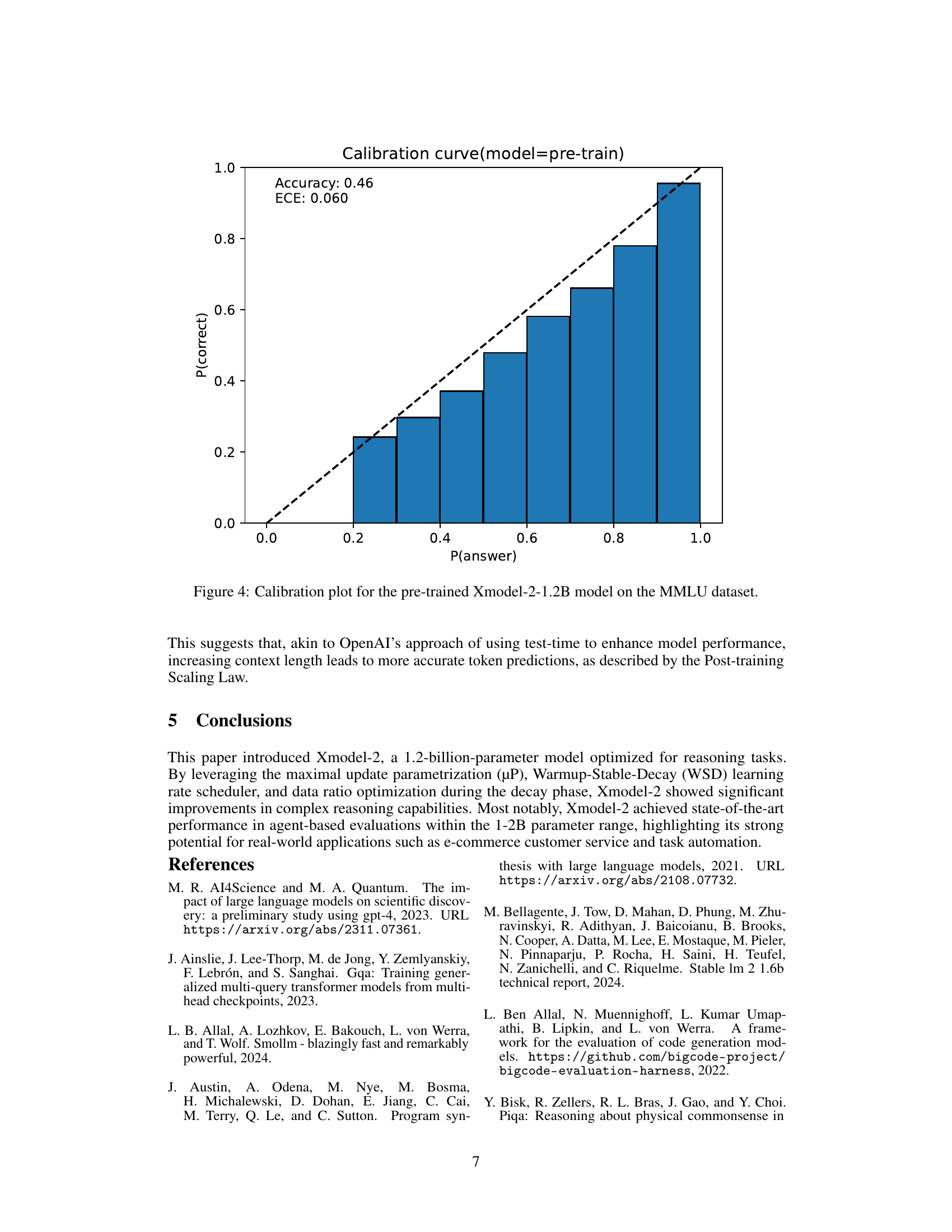
| Xmodel-2-1.2B | 13.70 | 40.00 | 0.78 | 2.20 | 14.21 |
🔼 This table presents the performance of various language models on four different agent-based tasks: HotpotQA, FEVER, AlfWorld, and WebShop. For HotpotQA and FEVER, the evaluation metric is Exact Match (EM), reflecting the percentage of questions answered perfectly. AlfWorld and WebShop use the success rate metric, measuring the proportion of attempts that successfully completed the given tasks. The results highlight the relative strengths and weaknesses of different models in handling complex reasoning, multi-step decision making, and real-world interactions within diverse agent environments.
read the caption
Table 4: Performance on Agent tasks.
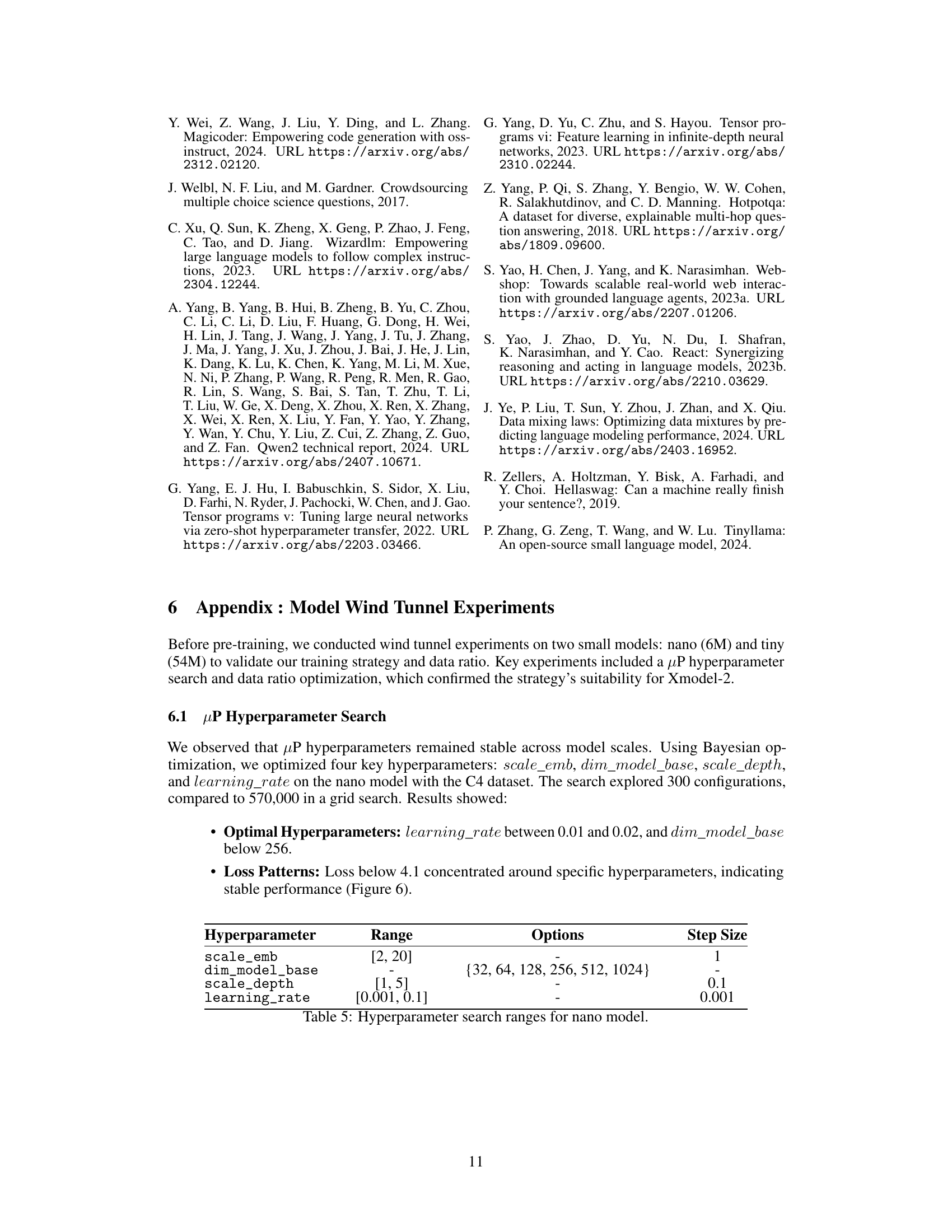
| Hyperparameter | Range | Options | Step Size |
|---|---|---|---|
scale_emb | [2, 20] | - | 1 |
dim_model_base | - | {32, 64, 128, 256, 512, 1024} | - |
scale_depth | [1, 5] | - | 0.1 |
learning_rate | [0.001, 0.1] | - | 0.001 |
🔼 This table details the ranges explored for each hyperparameter during the hyperparameter search for the nano model. The search was conducted to optimize the model’s performance. For each hyperparameter, the table shows the minimum and maximum values tested (Range), the specific values used in the search (Options), and the increment between values (Step Size). This information is crucial for understanding the optimization process and the range of values considered for each parameter to reach the optimal configuration for the nano model.
read the caption
Table 5: Hyperparameter search ranges for nano model.
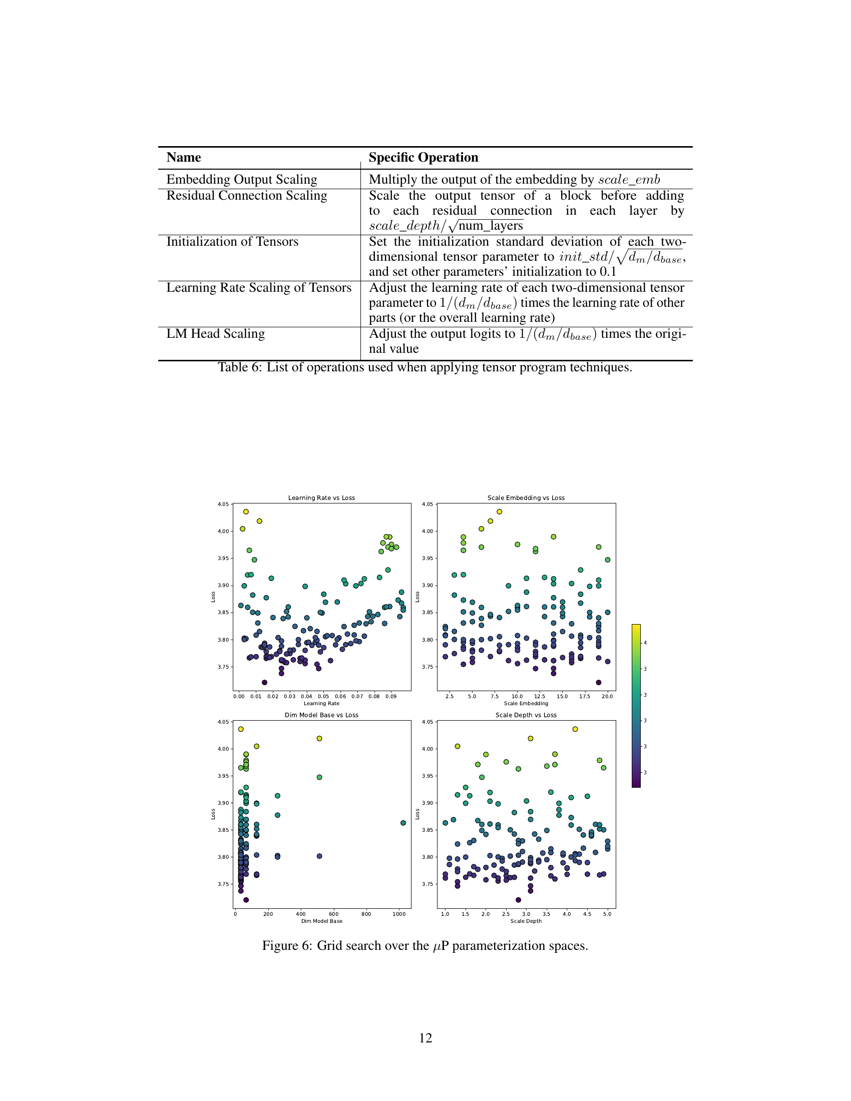
| Name | Specific Operation |
|---|---|
| Embedding Output Scaling | Multiply the output of the embedding by $scale_{emb}$ |
| Residual Connection Scaling | Scale the output tensor of a block before adding to each residual connection in each layer by $scale_{depth}/\sqrt{num_layers}$ |
| Initialization of Tensors | Set the initialization standard deviation of each two-dimensional tensor parameter to $init_std/\sqrt{d_{m}/d_{base}}$, and set other parameters’ initialization to 0.1 |
| Learning Rate Scaling of Tensors | Adjust the learning rate of each two-dimensional tensor parameter to $1/(d_{m}/d_{base})$ times the learning rate of other parts (or the overall learning rate) |
| LM Head Scaling | Adjust the output logits to $1/(d_{m}/d_{base})$ times the original value |
🔼 This table details the specific operations performed when applying tensor program techniques within the Xmodel-2 architecture. Each row represents a specific scaling or modification applied to different parts of the model, such as embedding outputs, residual connections, and tensor initializations. The ‘Specific Operation’ column describes precisely how each technique alters model parameters and learning rates to enhance efficiency and transferability across different model scales.
read the caption
Table 6: List of operations used when applying tensor program techniques.
Full paper#
