TL;DR#
State Space Models (SSMs), while promising for long-sequence processing, suffer from two key limitations: a strong recency bias, where the model prioritizes recent information, and over-smoothing, where deeper networks lose the ability to distinguish between tokens. These limitations hinder the model’s ability to recall distant information and make them vulnerable to adversarial attacks.
The researchers propose a novel “polarization” technique. This involves modifying the state transition matrices within the SSM to create two separate channels; one designed to preserve historical context and the other to suppress excessive smoothing. Experiments demonstrate that this technique consistently improves recall accuracy for long-range information, and it enables SSMs to benefit more significantly from deeper network architectures, thus overcoming the inherent limitations.
Key Takeaways#
Why does it matter?#
This paper is crucial for researchers working with state space models (SSMs) and sequence processing. It identifies critical limitations of existing SSMs, namely recency bias and over-smoothing, hindering their scalability. The proposed polarization technique offers a practical solution, opening new avenues for improving SSM performance and addressing robustness issues. This is highly relevant to current trends in efficient and long-context sequence modeling.
Visual Insights#

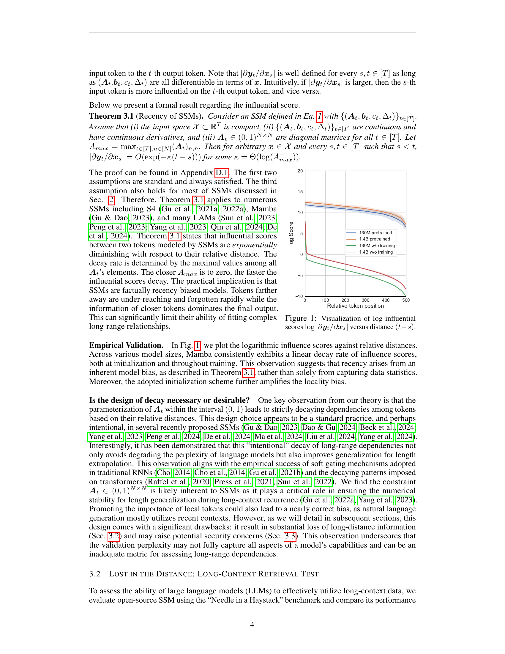
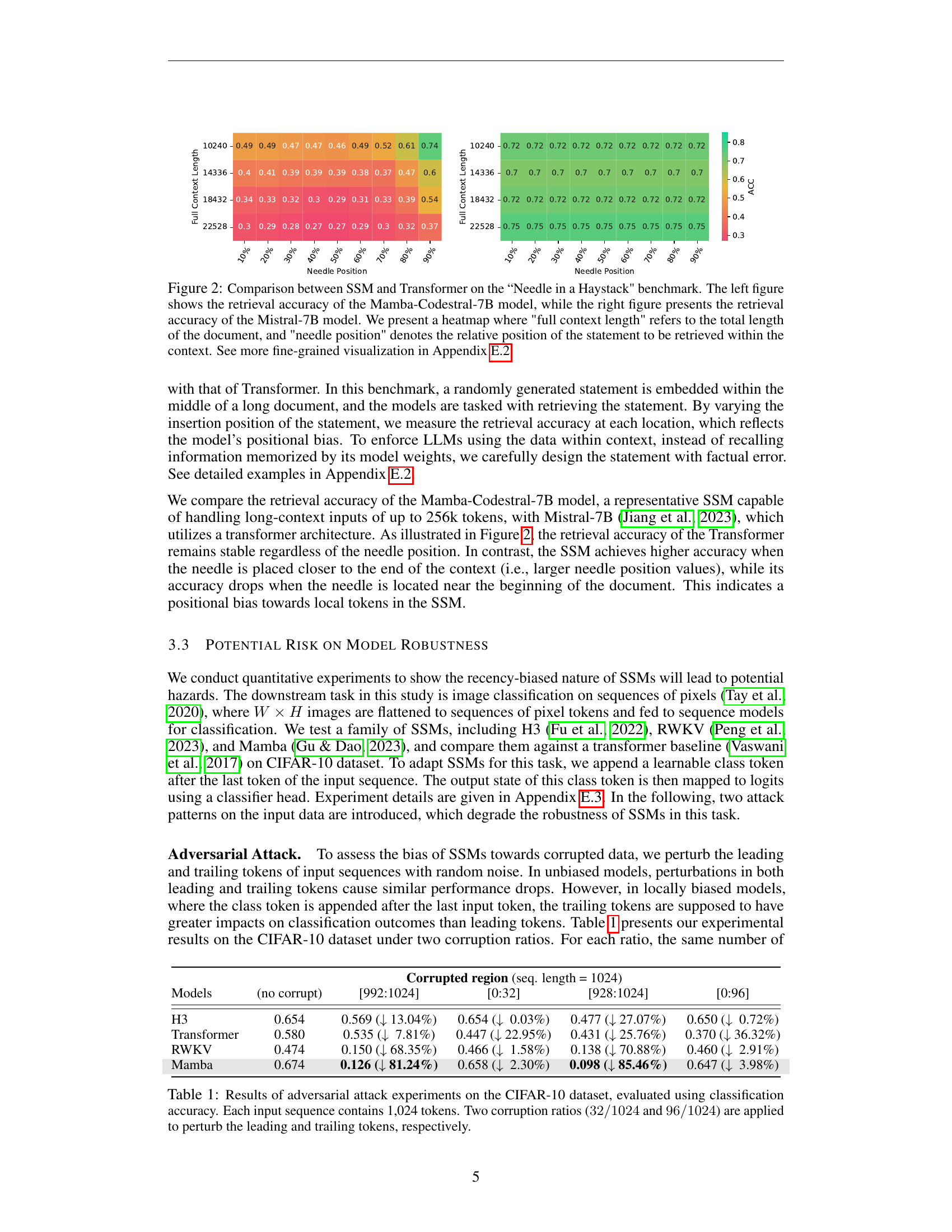
🔼 The figure visualizes the relationship between the logarithmic influence scores (log|∂yt/∂xs|) and the relative distance (t-s) between tokens in a sequence processed by a state space model (SSM). The influence score quantifies how much a given input token (xs) impacts a specific output token (yt). The plot shows how this influence decays exponentially with distance, illustrating the recency bias inherent in SSMs. Different lines represent different pre-trained SSM models (with varying sizes), and all show a consistent linear decay rate. This suggests the recency bias in SSMs is a property of the model architecture rather than merely a reflection of data statistics.
read the caption
Figure 1: Visualization of log influential scores log|∂𝒚t/∂𝒙s|subscript𝒚𝑡subscript𝒙𝑠\log|\partial\bm{y}_{t}/\partial\bm{x}_{s}|roman_log | ∂ bold_italic_y start_POSTSUBSCRIPT italic_t end_POSTSUBSCRIPT / ∂ bold_italic_x start_POSTSUBSCRIPT italic_s end_POSTSUBSCRIPT | versus distance (t−s)𝑡𝑠(t-s)( italic_t - italic_s ).
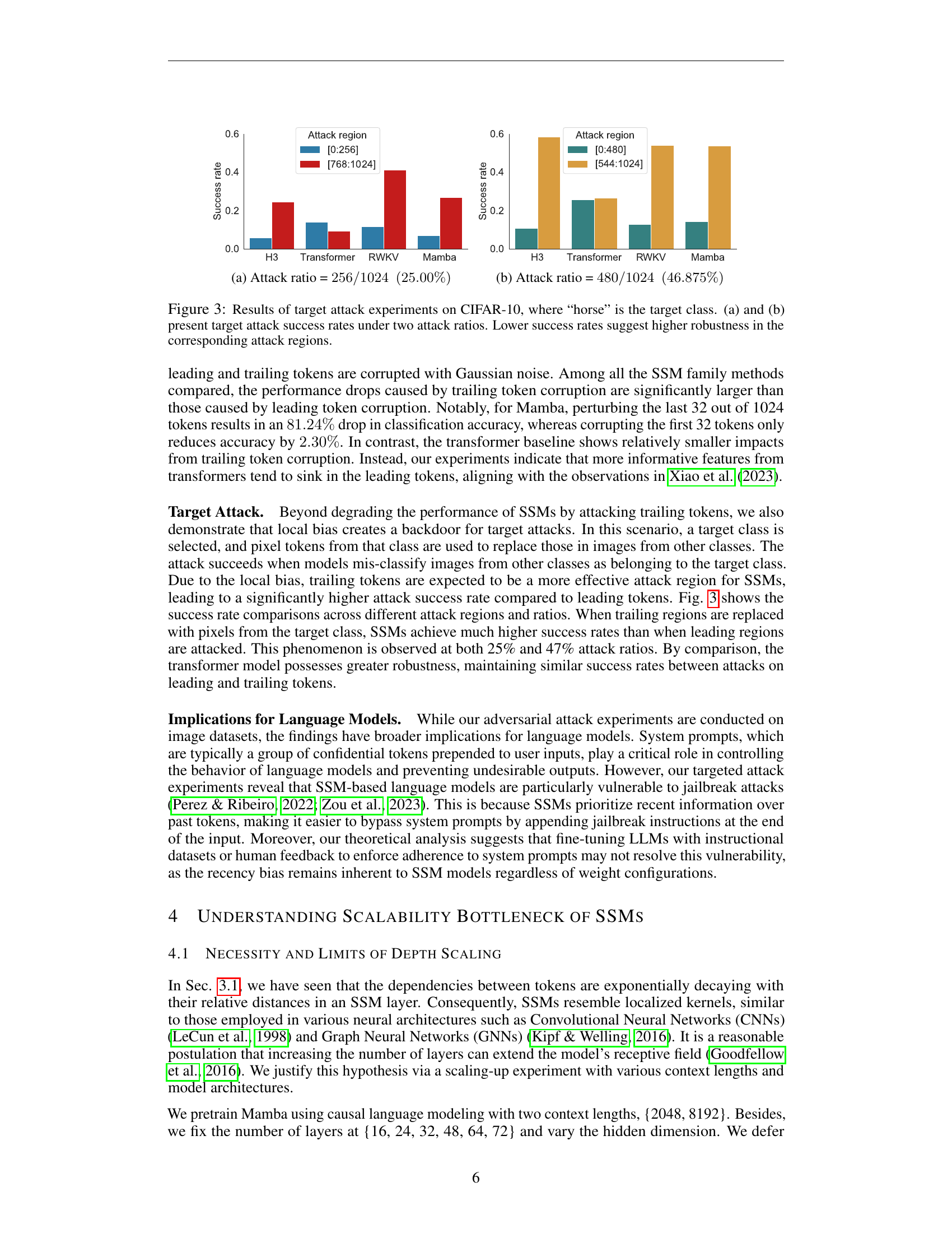
| Models | (no corrupt) | [992:1024] | [0:32] | [928:1024] | [0:96] |
|---|---|---|---|---|---|
| H3 | 0.654 | 0.569 (↓ 13.04%) | 0.654 (↓ 0.03%) | 0.477 (↓ 27.07%) | 0.650 (↓ 0.72%) |
| Transformer | 0.580 | 0.535 (↓ 7.81%) | 0.447 (↓ 22.95%) | 0.431 (↓ 25.76%) | 0.370 (↓ 36.32%) |
| RWKV | 0.474 | 0.150 (↓ 68.35%) | 0.466 (↓ 1.58%) | 0.138 (↓ 70.88%) | 0.460 (↓ 2.91%) |
| Mamba | 0.674 | 0.126 (↓ 81.24%) | 0.658 (↓ 2.30%) | 0.098 (↓ 85.46%) | 0.647 (↓ 3.98%) |
🔼 This table presents the results of adversarial attack experiments conducted on the CIFAR-10 dataset to evaluate the robustness of different sequence models. The models’ classification accuracy is measured after introducing perturbations to either the leading (beginning) or trailing (end) tokens of the input sequences. Two different levels of corruption are tested: 32 out of 1024 tokens are corrupted (3.125%) and 96 out of 1024 tokens (9.375%). The table allows comparison of the models’ vulnerability to these perturbations, highlighting the impact on the classification accuracy depending on where in the sequence the perturbations occur.
read the caption
Table 1: Results of adversarial attack experiments on the CIFAR-10 dataset, evaluated using classification accuracy. Each input sequence contains 1,024 tokens. Two corruption ratios (32/102432102432/102432 / 1024 and 96/102496102496/102496 / 1024) are applied to perturb the leading and trailing tokens, respectively.
In-depth insights#
SSM Recency Bias#
The concept of “SSM Recency Bias” highlights a critical limitation of Structured State Space Models (SSMs) in handling long-range dependencies within sequences. SSMs, while theoretically capable of capturing long-range information, exhibit a strong tendency to prioritize recent information over earlier context. This bias manifests as an exponential decay in the influence of earlier tokens on later predictions, hindering the model’s ability to effectively recall distant information. The paper reveals that this recency bias stems from the inherent mathematical properties of SSMs and not merely from data limitations or model architecture choices. This recency is further amplified by the design and parameterization choices commonly used in practice. This bias negatively impacts the model’s robustness, making it susceptible to adversarial attacks targeting the manipulation of earlier less influential tokens. Therefore, understanding and mitigating this inherent bias is crucial for improving SSMs’ ability to fully exploit long sequences, enhancing their performance and addressing security concerns.
Over-smoothing Issue#
The over-smoothing issue, as discussed in the context of state-space models (SSMs), describes the phenomenon where, as SSMs increase in depth, token representations become increasingly indistinguishable. This is a critical limitation because it hinders the SSM’s ability to effectively represent and utilize long-range dependencies. The core problem is that SSMs act as smoothing operators, progressively blurring distinctions between tokens. This effect is exacerbated in deeper models leading to a performance plateau and eventual decline in performance. The paper highlights that the fundamental dilemma between recency bias and over-smoothing is a major obstacle to scaling SSMs. The over-smoothing effect is directly linked to the nature of the state transition matrices and the recurrent updates. The proposed solution, polarization, aims to tackle both issues simultaneously by introducing carefully chosen fixed values in the state transition matrices to control the degree of smoothing and retain memory information effectively.
Polarization Method#
The proposed “Polarization Method” addresses the inherent limitations of Structured State Space Models (SSM) by directly tackling their recency bias and over-smoothing tendencies. The core idea is to strategically modify the state transition matrices of the SSM. Specifically, it involves polarizing two channels within these matrices, forcing one channel to always retain past information (by setting its values to 1) and another to only focus on the current token (by setting its values to 0). This dual-channel approach cleverly balances the model’s ability to learn from long-range dependencies (via the persistent channel) and prevents the complete loss of fine-grained, recent details (via the zeroed-out channel). This avoids the inherent trade-off between capturing long-range contexts and maintaining sensitivity to recent inputs, a significant limitation found in other SSM architectures. The method’s effectiveness is empirically demonstrated through improved recall accuracy in long-range association tasks, showcasing its potential for enhancing the performance of SSMs and making them more robust and less susceptible to adversarial attacks.
Depth Scaling Limits#
The concept of “Depth Scaling Limits” in the context of state space models (SSMs) for sequence processing highlights a critical trade-off between model capacity and performance. While increasing the depth of SSMs initially improves the ability to capture long-range dependencies, this improvement plateaus and eventually reverses at a certain depth. This limitation stems from the inherent smoothing nature of SSMs, where token representations become increasingly similar as the depth increases, leading to a phenomenon known as over-smoothing. This over-smoothing effect diminishes the discriminative power of the model, hindering its ability to distinguish between meaningful and irrelevant information in long sequences. The depth at which the over-smoothing effect dominates depends on factors such as the context length of the input sequences and the specific SSM architecture. Therefore, optimizing the depth of SSMs requires careful consideration of the specific application and dataset, aiming for a balance between sufficient capacity to capture long-range interactions and preventing the detrimental effects of over-smoothing. Furthermore, techniques to mitigate over-smoothing, such as the proposed polarization method, may be crucial for effectively scaling SSM depth and unlocking their full potential in modeling complex sequences.
Future Work#
Future research directions stemming from this paper could explore several promising avenues. Extending the polarization technique to other SSM architectures beyond Mamba, and rigorously evaluating its effectiveness across diverse tasks and datasets is crucial. Investigating the interaction between polarization and other SSM design choices, like the selection mechanism or the type of activation functions, would provide a deeper understanding of its impact on model performance. Further theoretical analysis could focus on generalizing the over-smoothing and recency bias theorems to a wider class of SSMs and even other sequence models to uncover more universal principles governing sequence processing. Developing more sophisticated methods for mitigating over-smoothing, beyond simple polarization, could involve exploring alternative state space transformations or incorporating attention mechanisms selectively to control information flow. Finally, empirical studies examining the robustness of polarized SSMs against various adversarial attacks and their potential for improved generalization in low-resource settings would significantly increase our confidence in the proposed solution’s practical applicability.
More visual insights#
More on figures

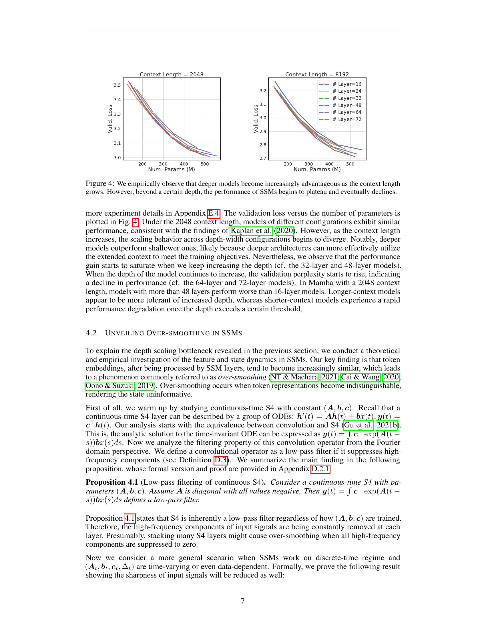
🔼 This figure compares the performance of State Space Models (SSMs) and Transformers on the ‘Needle in a Haystack’ benchmark, a task designed to evaluate the ability of language models to retrieve information from long contexts. The benchmark involves embedding a statement within a long document and assessing the model’s ability to retrieve that statement. The left heatmap shows the results for the Mamba-Codestral-7B SSM, while the right heatmap shows the results for the Mistral-7B Transformer model. The heatmaps illustrate retrieval accuracy across different document lengths (‘full context length’) and statement positions within the document (’needle position’). The results reveal a recency bias in the SSM, where accuracy is higher when the statement is closer to the end of the document. The Transformer model shows more consistent performance regardless of statement position.
read the caption
Figure 2: Comparison between SSM and Transformer on the “Needle in a Haystack' benchmark. The left figure shows the retrieval accuracy of the Mamba-Codestral-7B model, while the right figure presents the retrieval accuracy of the Mistral-7B model. We present a heatmap where 'full context length' refers to the total length of the document, and 'needle position' denotes the relative position of the statement to be retrieved within the context. See more fine-grained visualization in Appendix E.2.

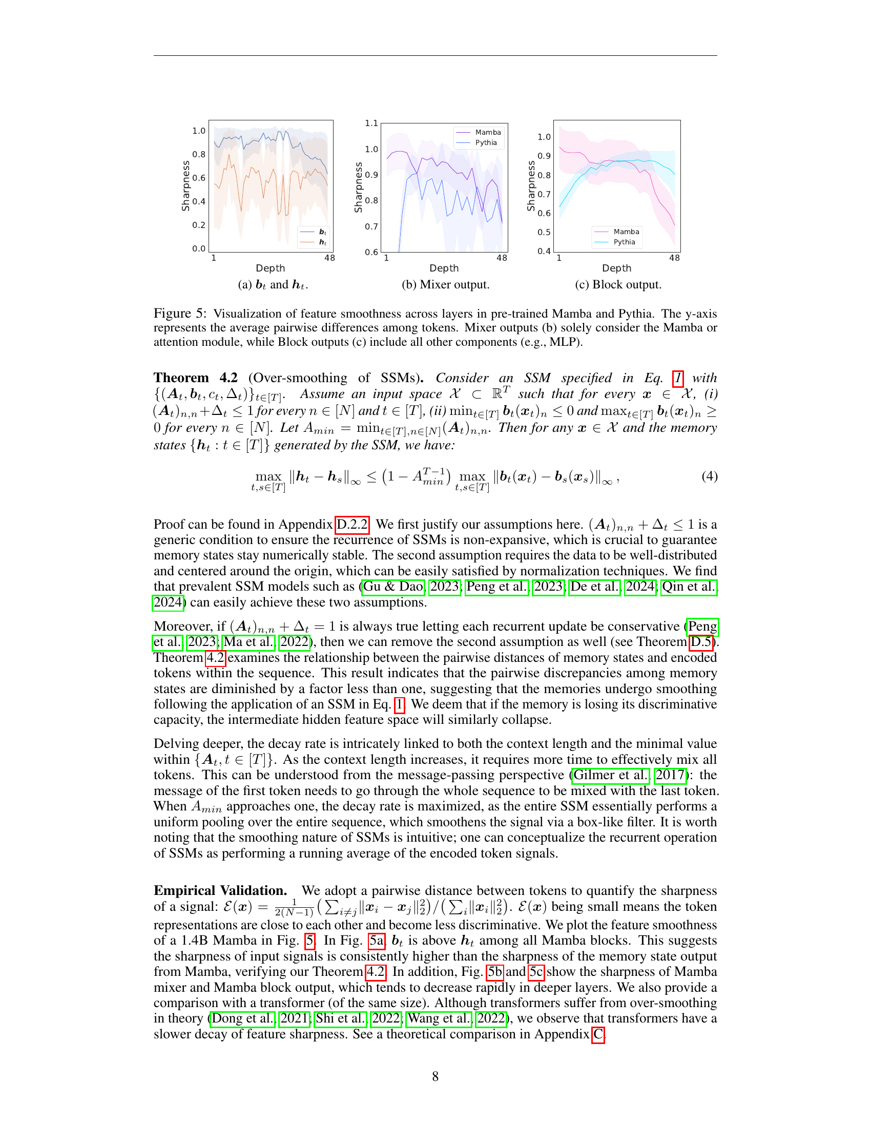
🔼 This figure shows the results of a target attack experiment on the CIFAR-10 dataset, focusing on the impact of attacking different regions of the input sequences on model performance. Two attack ratios are shown: 25.00% and 46.875%. Each bar represents the attack success rate for a specific model (H3, Transformer, RWKV, Mamba) and attack region (leading or trailing tokens). Lower success rates indicate higher robustness against that type of attack.
read the caption
(a) Attack ratio = 256/1024(25.00%)2561024percent25.00256/1024~{}~{}(25.00\%)256 / 1024 ( 25.00 % )

🔼 This figure shows the results of a target attack experiment on the CIFAR-10 dataset. Specifically, it shows the attack success rates for different models (H3, Transformer, RWKV, Mamba) when a significant portion (46.875%) of the input sequence is replaced with pixels from the target class. This is done separately for leading and trailing tokens, illustrating model vulnerability to targeted attacks. Lower success rates indicate higher robustness.
read the caption
(b) Attack ratio = 480/1024(46.875%)4801024percent46.875480/1024~{}~{}(46.875\%)480 / 1024 ( 46.875 % )

🔼 This figure displays the results of targeted attack experiments conducted on the CIFAR-10 dataset, focusing on the robustness of different models against adversarial attacks. The target class for these attacks was ‘horse’. Two attack scenarios were tested, each with different ratios of corrupted data: (a) 25% and (b) 47%. The attacks involved replacing pixels in either the beginning or end of the image sequences with pixels from images of the target class. The success rate of the attack (how often the model misclassified a non-horse image as a horse) is shown for four models: H3, Mamba, RWKV and the Transformer baseline. Lower success rates indicate greater robustness of the model to that type of attack. The figure shows that SSMs (H3, Mamba, and RWKV) are significantly less robust to attacks targeting trailing tokens (the end of the sequence), while the Transformer is less susceptible to either leading or trailing token attacks.
read the caption
Figure 3: Results of target attack experiments on CIFAR-10, where “horse” is the target class. (a) and (b) present target attack success rates under two attack ratios. Lower success rates suggest higher robustness in the corresponding attack regions.

🔼 This figure displays the validation loss of the Mamba model across different numbers of layers and model sizes (number of parameters) for two different context lengths (2048 and 8192). It demonstrates that increasing model depth improves performance, particularly as context length increases. However, beyond a certain number of layers (depth), the performance plateaus and then starts to decrease, indicating a scalability bottleneck in SSMs at greater depths.
read the caption
Figure 4: We empirically observe that deeper models become increasingly advantageous as the context length grows. However, beyond a certain depth, the performance of SSMs begins to plateau and eventually declines.

🔼 The figure visualizes the feature smoothness across layers in pre-trained Mamba and Pythia models. Panel (a) shows the sharpness of the input features (𝑏𝑡) and the hidden states (ℎ𝑡). Panel (b) focuses only on the mixer module output, while panel (c) shows the output of the entire block, encompassing all components (mixer, MLP, etc.). The y-axis represents the average pairwise difference between tokens; a lower value signifies greater feature smoothness and thus more oversmoothing.
read the caption
(a) 𝒃tsubscript𝒃𝑡\bm{b}_{t}bold_italic_b start_POSTSUBSCRIPT italic_t end_POSTSUBSCRIPT and 𝒉tsubscript𝒉𝑡\bm{h}_{t}bold_italic_h start_POSTSUBSCRIPT italic_t end_POSTSUBSCRIPT.

🔼 This figure shows the sharpness of features in the output of the mixer module in Mamba and Pythia models. Sharpness is a measure of how distinguishable the token representations are; lower sharpness indicates over-smoothing, where token representations become too similar.
read the caption
(b) Mixer output.

🔼 This figure visualizes the feature smoothness across layers in pre-trained Mamba and Pythia models. The y-axis represents the average pairwise differences among tokens. The figure displays smoothness for three different output types: (a) the input tokens (bt) and hidden state (ht) vectors, (b) the output of the attention module (mixer), and (c) the output of the entire block (block), which encompasses all components within a single block of the model architecture. Comparing across these output types allows for analysis of how smoothness changes as information flows through different stages of the model.
read the caption
(c) Block output.

🔼 This figure visualizes how feature smoothness changes across different layers of pre-trained Mamba and Pythia language models. Feature smoothness is measured as the average pairwise difference between token representations. The figure includes three sub-figures. (a) shows the smoothness of the input token embeddings (bt) and the hidden state representations (ht) at each layer. (b) focuses on the smoothness of the output from the Mamba or attention module (mixer) only. (c) shows the overall smoothness of the output of the entire block, including all components like MLPs in addition to the attention/Mamba module. This allows for a comparison of smoothness within the attention module and the overall effect of the entire block on the features. This helps to understand the impact of various model components on feature over-smoothing.
read the caption
Figure 5: Visualization of feature smoothness across layers in pre-trained Mamba and Pythia. The y-axis represents the average pairwise differences among tokens. Mixer outputs (b) solely consider the Mamba or attention module, while Block outputs (c) include all other components (e.g., MLP).

🔼 This figure shows the cumulative distribution of the difference between the maximum and minimum values of the diagonal elements of the state transition matrix (A) across different channels in the SSM model. The x-axis represents the threshold for the difference (A_max - A_min), while the y-axis shows the cumulative percentage of channels where the difference is less than or equal to the threshold. This distribution reveals that a significant proportion of channels do not exhibit a large difference between maximum and minimum values, which is an indicator that simultaneous mitigation of recency bias and over-smoothing is challenging.
read the caption
Figure 6: Cumulative histogram of (Amax−Amin)subscript𝐴𝑚𝑎𝑥subscript𝐴𝑚𝑖𝑛(A_{max}-A_{min})( italic_A start_POSTSUBSCRIPT italic_m italic_a italic_x end_POSTSUBSCRIPT - italic_A start_POSTSUBSCRIPT italic_m italic_i italic_n end_POSTSUBSCRIPT ). The height of each bin represents the cumulative proportion of (Amax−Amin)subscript𝐴𝑚𝑎𝑥subscript𝐴𝑚𝑖𝑛(A_{max}-A_{min})( italic_A start_POSTSUBSCRIPT italic_m italic_a italic_x end_POSTSUBSCRIPT - italic_A start_POSTSUBSCRIPT italic_m italic_i italic_n end_POSTSUBSCRIPT ) less than or equal to the corresponding value on the x-axis.
More on tables
| Configurations | # Layers | # KV Pairs | # KV Pairs | # KV Pairs | Avg. |
|---|---|---|---|---|---|
| 64 | 128 | 256 | |||
| Default At | 2 | 98.38 | 81.81 | 36.00 | 72.06 |
| Default At | 4 | 99.23 | 82.08 | 33.52 | 71.61 |
| (At)1,1=1 | 2 | 99.81 | 94.70 | 56.39 | 83.63 |
| (At)N,N=0 | 2 | 98.41 | 81.35 | 36.55 | 72.10 |
| (At)N,N=0 | 4 | 99.74 | 92.20 | 52.21 | 81.38 |
| (At)1,1=1,(At)N,N=0 | 2 | 99.23 | 95.54 | 54.74 | 83.17 |
| (At)1,1=1,(At)N,N=0 | 4 | 99.94 | 98.80 | 81.56 | 93.43 |
🔼 This table presents the results of an experiment evaluating the impact of a technique called ‘polarization’ on the performance of a state space model (SSM). The polarization technique involves modifying the state transition matrices of the SSM by setting specific channels to either 0 or 1. The table compares the performance (likely measured by a metric such as accuracy or loss) across different configurations: no polarization, polarization of one channel to 0, polarization of one channel to 1, and polarization of both channels (one to 0 and one to 1). Each configuration is tested with varying depths (# layers) and numbers of key-value pairs used in the training data. This allows for an assessment of how the polarization method affects performance under different conditions.
read the caption
Table 2: Results of polarization. Rows 1-2 have no polarization, rows 3-5 only polarize one channel to either one or zero, and rows 6-7 polarize both channels.
| Models | (no corrupt) | [1014:1024] | [0:10] | [768:1024] | [0:256] | [512:544] | [480:576] |
|---|---|---|---|---|---|---|---|
| H3 | 0.654 | 0.629 | 0.654 | 0.394 | 0.639 | 0.603 | 0.543 |
| Transformer | 0.580 | 0.571 | 0.500 | 0.249 | 0.263 | 0.498 | 0.347 |
| RWKV | 0.474 | 0.194 | 0.470 | 0.107 | 0.448 | 0.405 | 0.392 |
| Mamba | 0.674 | 0.348 | 0.664 | 0.099 | 0.597 | 0.515 | 0.446 |
🔼 This table presents the results of adversarial attack experiments conducted on the CIFAR-10 image classification dataset. It evaluates the robustness of several different sequence models (H3, Transformer, RWKV, Mamba) against two types of adversarial attacks: (1) corruption of leading and trailing tokens using Gaussian noise and (2) targeted attacks where pixels from a target class are inserted into images from different classes. The table shows classification accuracy under various corruption ratios, comparing the resilience of each model to both attack methods.
read the caption
Table 3: Extended results of adversarial attack experiments on the CIFAR-10 dataset. Classification accuracy is used as the metric.
| # Params | Training steps | Peak LR | Batch Size (in tokens) | # Tokens |
|---|---|---|---|---|
| 100-250M | 4800 | 3e-3 | 0.5M | 2.5B |
| 250-400M | 13500 | 1.5e-3 | 0.5M | 7B |
| 400-550M | 20000 | 1.25e-3 | 0.5M | 10B |
🔼 This table details the hyperparameters used during the training of various sized Mamba models. It shows how parameters like the number of training steps, peak learning rate, batch size, and the total number of tokens used varied depending on the model’s size (measured in the number of parameters). The settings were chosen to align with the Chinchilla scaling laws proposed by Hoffmann et al. (2022) and are consistent with the training methodology described by Gu & Dao (2023).
read the caption
Table 4: Summary of training settings for varying-sized Mamba. The settings are following Chinchilla law (Hoffmann et al., 2022) and consistent with Gu & Dao (2023).
🔼 Table 5 expands on the results presented in Table 5 of the paper by examining the effects of different configurations on locality and over-smoothing in the context of associative recall. It shows that a combination of 1-polarization (setting one channel of the state transition matrix to 1) and 0-polarization (setting another channel to 0) significantly mitigates locality issues, while deepening the architecture primarily helps reduce recency bias without worsening over-smoothing. Importantly, 0-polarization alone effectively reduces over-smoothing, enabling improved performance gains from increased depth.
read the caption
Table 5: Extension to Tab. 5. We note the extent of locality and over-smoothing for each configuration. We consider 1111-polarization mitigates locality most significantly, while deepening architecture only relieves recency mildly but deteriorates over-smoothing. 00-polarization alleviates over-smoothening and unleash the benefits by depth scaling.
Full paper#
