↗ arXiv ↗ Hugging Face ↗ Papers with Code
TL;DR#
Current genomic models often focus on curated datasets from specific species, limiting their ability to analyze the complex diversity of the microbiome. Moreover, tracking pathogen prevalence in wastewater requires analyzing massive datasets which requires efficient and robust model. This lack of comprehensive models hinders effective pandemic monitoring and early detection of emerging threats.
The researchers introduce METAGENE-1, a large language model trained on a vast, novel dataset of human wastewater metagenomic sequences. This model outperforms existing methods on key benchmarks for pathogen detection and genomic embedding, showcasing its potential for pandemic monitoring and biosurveillance. The open-sourcing of METAGENE-1 and its code facilitates broader research and development in the field.
Key Takeaways#
Why does it matter?#
This paper is crucial for researchers in metagenomics, public health, and machine learning. It introduces a novel foundation model, METAGENE-1, trained on a massive wastewater metagenomic dataset. This opens new avenues for pathogen detection, biosurveillance, and developing advanced genomic analysis tools. Its innovative approach and strong empirical results will significantly influence future research in these areas. The open-sourcing of the model and code further enhances its impact on the research community.
Visual Insights#

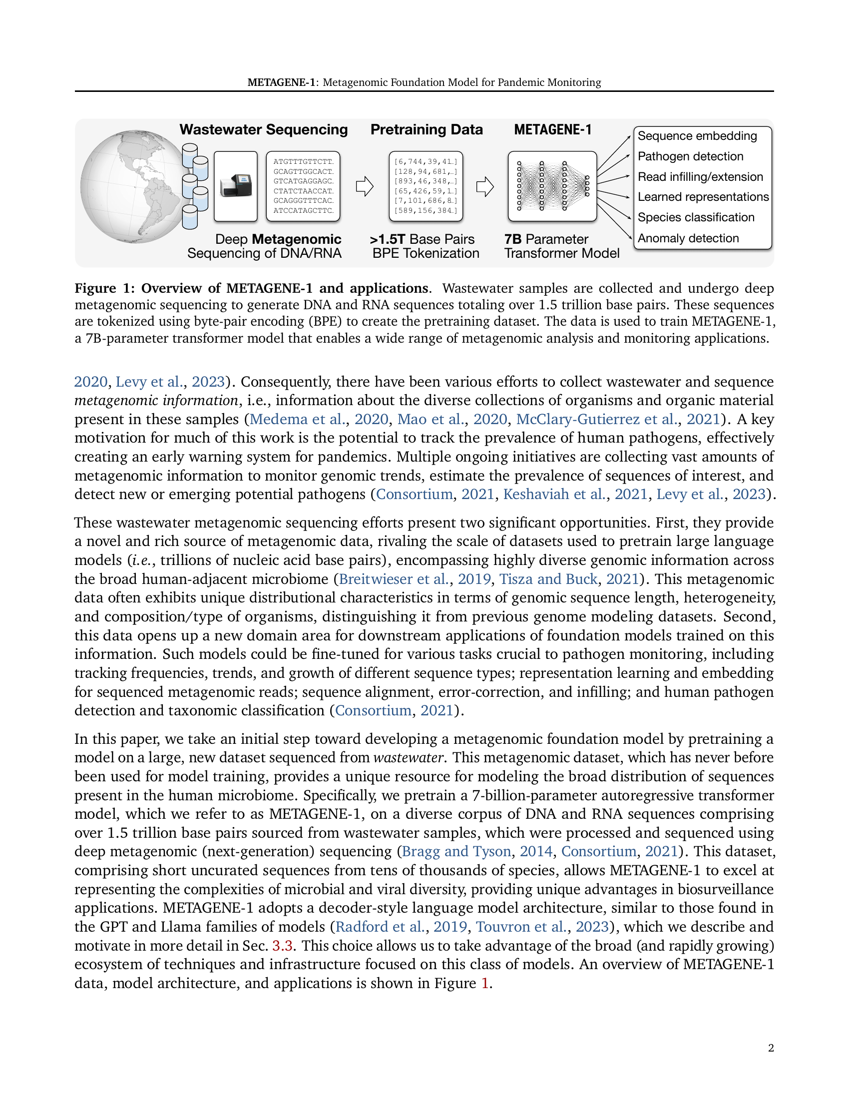
🔼 The figure illustrates the workflow of METAGENE-1, a metagenomic foundation model. It begins with the collection of wastewater samples, which are then subjected to deep metagenomic sequencing to produce a massive dataset of over 1.5 trillion DNA and RNA base pairs. This raw sequence data undergoes byte-pair encoding (BPE) tokenization to create the pretraining dataset for the 7-billion parameter transformer model, METAGENE-1. Finally, the trained METAGENE-1 model is shown to be applicable to a wide range of metagenomic analyses and monitoring tasks.
read the caption
Figure 1: Overview of METAGENE-1 and applications. Wastewater samples are collected and undergo deep metagenomic sequencing to generate DNA and RNA sequences totaling over 1.5 trillion base pairs. These sequences are tokenized using byte-pair encoding (BPE) to create the pretraining dataset. The data is used to train METAGENE-1, a 7B-parameter transformer model that enables a wide range of metagenomic analysis and monitoring applications.
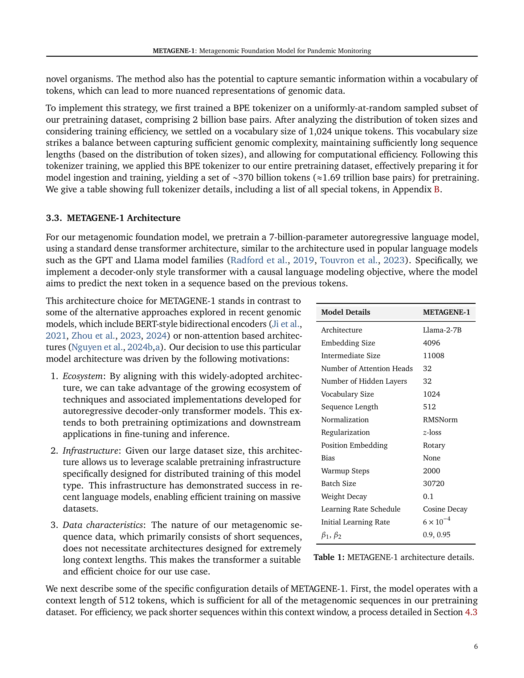
| Model Details | METAGENE-1 |
|---|---|
| Architecture | Llama-2-7B |
| Embedding Size | 4096 |
| Intermediate Size | 11008 |
| Number of Attention Heads | 32 |
| Number of Hidden Layers | 32 |
| Vocabulary Size | 1024 |
| Sequence Length | 512 |
| Normalization | RMSNorm |
| Regularization | z-loss |
| Position Embedding | Rotary |
| Bias | None |
| Warmup Steps | 2000 |
| Batch Size | 30720 |
| Weight Decay | 0.1 |
| Learning Rate Schedule | Cosine Decay |
| Initial Learning Rate | 6 × 10⁻⁴ |
| β1, β2 | 0.9, 0.95 |
🔼 This table provides detailed specifications of the METAGENE-1 architecture, including the model type (autoregressive transformer), embedding size, number of attention heads, hidden layer size, normalization method, regularization type, positional embedding technique, bias usage, warmup steps, batch size, weight decay, learning rate schedule, initial learning rate, and beta parameters (β1, β2). It compares these hyperparameters to those of the Llama-2-7B model for context and shows the overall model size.
read the caption
Table 1: METAGENE-1 architecture details.
In-depth insights#
Metagenomic Dataset#
The section on “Metagenomic Dataset” would be crucial in evaluating the paper’s methodology and results. It should detail the origin and scale of the dataset, specifying the source (human wastewater), the sequencing technology used (e.g., Illumina), and the total volume of data (e.g., base pairs or reads). The description must address the diversity of the dataset—does it represent a broad range of organisms and genetic material or is it biased? The authors should justify their choice of wastewater as a data source, discussing the potential advantages and limitations of this approach, including considerations of bias and contamination. Furthermore, it should mention data pre-processing steps, such as quality control, filtering, and read assembly. A discussion on how these steps impacted the final dataset’s characteristics and the potential for introducing biases is crucial. Finally, the paper must acknowledge the ethical considerations regarding the use of wastewater samples and explain how data privacy was addressed.
Model Architecture#
The research paper’s description of the model architecture is crucial for understanding its capabilities and limitations. A 7-billion parameter autoregressive transformer model is employed, akin to the architecture of well-known language models. The choice of a decoder-only style transformer with a causal language modeling objective suggests a focus on generating sequences rather than bidirectional understanding. This is particularly relevant given the nature of the metagenomic data, which consists of sequences of varying lengths and compositions. The use of byte-pair encoding (BPE) tokenization allows for flexible token lengths, accommodating the inherent variability of metagenomic data and allowing effective handling of novel or unknown sequences. This model design is further strengthened by the attention mechanism within the transformer, enabling the model to focus on relevant parts of the sequences during processing. The specific hyperparameter choices, like embedding size, the number of layers and attention heads, significantly influence the model’s performance. The choice to pack shorter sequences to utilize the full context length illustrates an optimization strategy reflecting the practical challenges associated with handling such diverse data. Finally, while the architecture is inspired by existing successful models, the adaptation for metagenomic data and the specific design choices made represent a novel contribution, enhancing the model’s ability to effectively learn from the unique challenges of this data domain.
Benchmark Results#
The benchmark results section of this metagenomic foundation model research paper would ideally present a comprehensive evaluation across multiple tasks, comparing METAGENE-1’s performance against existing state-of-the-art models. Key benchmarks should include pathogen detection, where the model’s accuracy in identifying known pathogens from metagenomic sequences would be a critical measure of success. Further, genomic sequence embedding benchmarks would showcase the model’s ability to generate effective vector representations of sequences, essential for downstream applications. Quantitative metrics like precision, recall, F1-score, and Matthews Correlation Coefficient (MCC) should be reported, along with statistical significance tests to confirm the improvements. An analysis of the model’s performance across various data subsets would reveal its generalization capabilities and robustness. Specific attention should be given to whether the model excels in handling the diversity and noise often present in real-world metagenomic data, thus demonstrating its practical applicability for pandemic monitoring and public health. Finally, a discussion of the limitations and potential sources of bias within the benchmarks, along with suggestions for future improvements, would greatly enhance the validity and impact of the findings.
Training Stability#
Training large language models, especially those with billions of parameters like the metagenomic foundation model METAGENE-1, presents significant challenges to stability. Instability often manifests as sudden spikes in loss or divergent behavior, potentially wasting considerable compute resources. The authors acknowledge the heightened risk of instability in training on metagenomic sequences compared to natural language due to the unique characteristics of this data. To mitigate this, they employed best practices, including a variant of z-loss, and carefully monitored key metrics such as gradient norms and layer normalizations. These measures, coupled with a hybrid sharding strategy for efficient GPU utilization, enabled them to maintain training stability despite encountering several node and GPU failures, emphasizing the importance of proactive strategies and robust infrastructure in training large-scale models. The relatively smooth loss curves shown suggest the effectiveness of their approach but highlight the ongoing challenges in training large, complex models on novel data types.
Future Directions#
The ‘Future Directions’ section of a metagenomic foundation model research paper would naturally focus on expanding the model’s capabilities and addressing its limitations. Improving the model’s interpretability is key; techniques like sparse autoencoders could help decipher the model’s internal representations, making its predictions more transparent and trustworthy. Addressing the current model’s limitations, such as its reliance on short-read sequences, is crucial. This could involve incorporating long-read data or exploring alternative architectural designs better suited for diverse sequence lengths. Incorporating more diverse and comprehensive data from a wider range of sources (e.g., beyond wastewater) will enrich the model and enable applications in varied environments and conditions. Exploring different pretraining objectives beyond language modeling, such as contrastive learning or other representation learning methods, could enhance its generalization and performance on downstream tasks. Finally, standardizing evaluation metrics for metagenomic models is necessary to facilitate fair comparison and progress tracking. The development of a comprehensive benchmark suite with tasks encompassing classification, embedding, anomaly detection, and pandemic monitoring would be a significant contribution to the field. Such a suite would also require robust evaluation procedures that are capable of assessing the reliability and safety of future models.
More visual insights#
More on figures

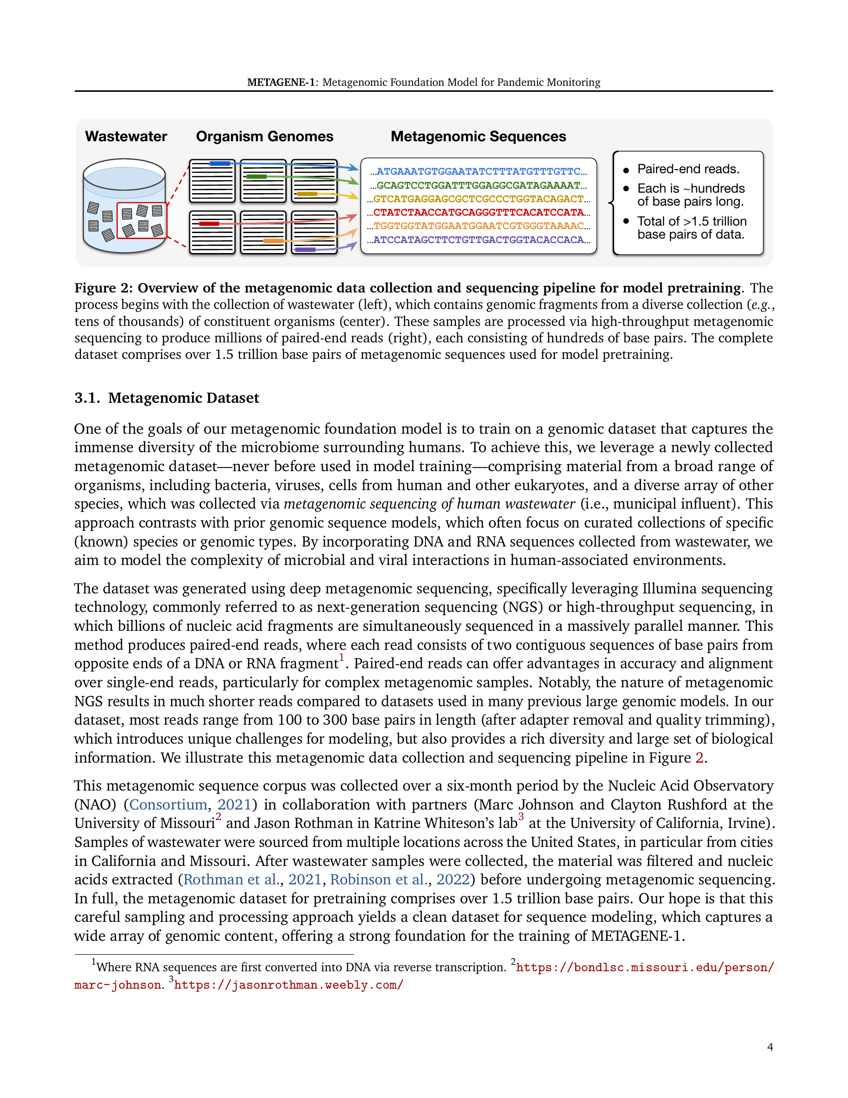
🔼 Figure 2 illustrates the process of creating the metagenomic dataset used to train the METAGENE-1 model. Starting with wastewater samples (left), which naturally contain DNA and RNA from diverse organisms (center, e.g., bacteria, viruses, human, etc.), high-throughput sequencing is applied. This generates millions of paired-end reads (right), each several hundred base pairs long. The combined length of these sequences in the final dataset exceeds 1.5 trillion base pairs.
read the caption
Figure 2: Overview of the metagenomic data collection and sequencing pipeline for model pretraining. The process begins with the collection of wastewater (left), which contains genomic fragments from a diverse collection (e.g., tens of thousands) of constituent organisms (center). These samples are processed via high-throughput metagenomic sequencing to produce millions of paired-end reads (right), each consisting of hundreds of base pairs. The complete dataset comprises over 1.5 trillion base pairs of metagenomic sequences used for model pretraining.

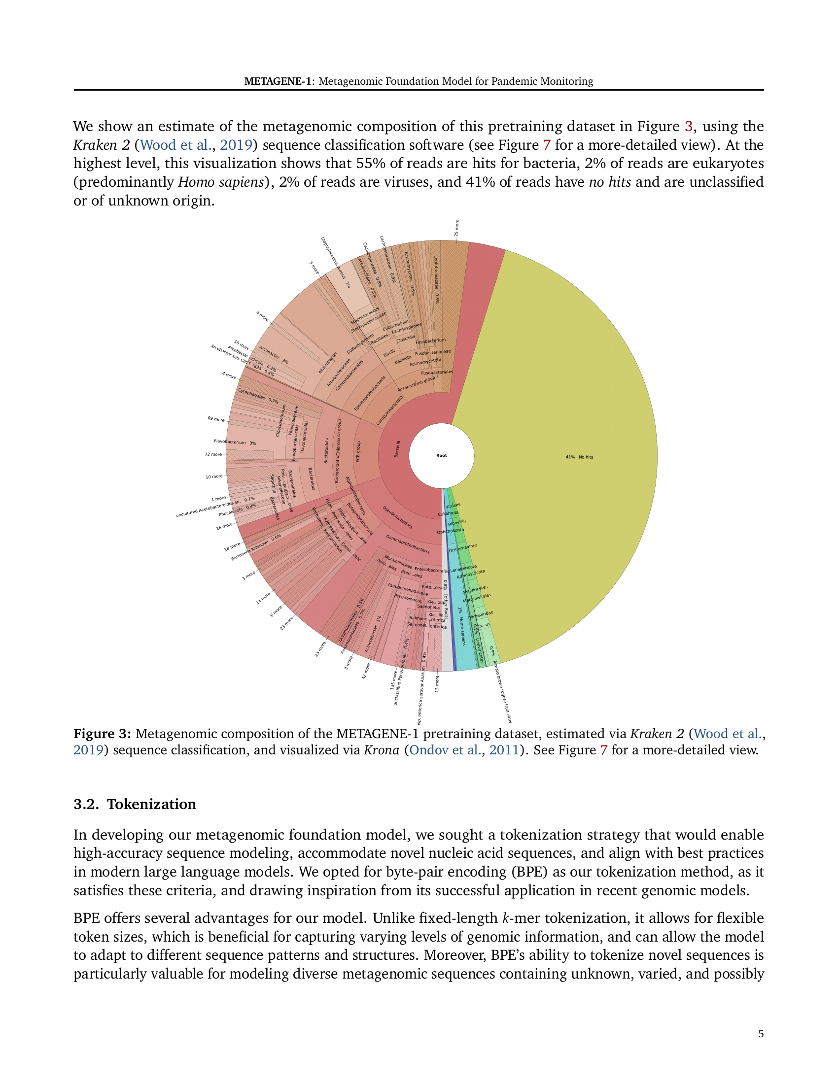
🔼 This figure is a visualization of the taxonomic composition of the metagenomic dataset used to pretrain the METAGENE-1 model. The dataset was analyzed using Kraken 2 software, which identifies the taxonomic origin of short sequences (reads) by comparing them to a database of known organisms. The resulting taxonomic assignments are displayed using the Krona software for visualization as a treemap. The visualization shows the relative abundance of different taxonomic groups present in the dataset, including bacteria, viruses, eukaryotes (mainly Homo sapiens), and unclassified sequences. The visualization highlights the high diversity and complexity of the metagenomic data, which is typical of wastewater samples and comprises a range of organisms, making it suitable for training a general-purpose foundation model.
read the caption
Figure 3: Metagenomic composition of the METAGENE-1 pretraining dataset, estimated via Kraken 2 (Wood et al., 2019) sequence classification, and visualized via Krona (Ondov et al., 2011). See Figure 7 for a more-detailed view.

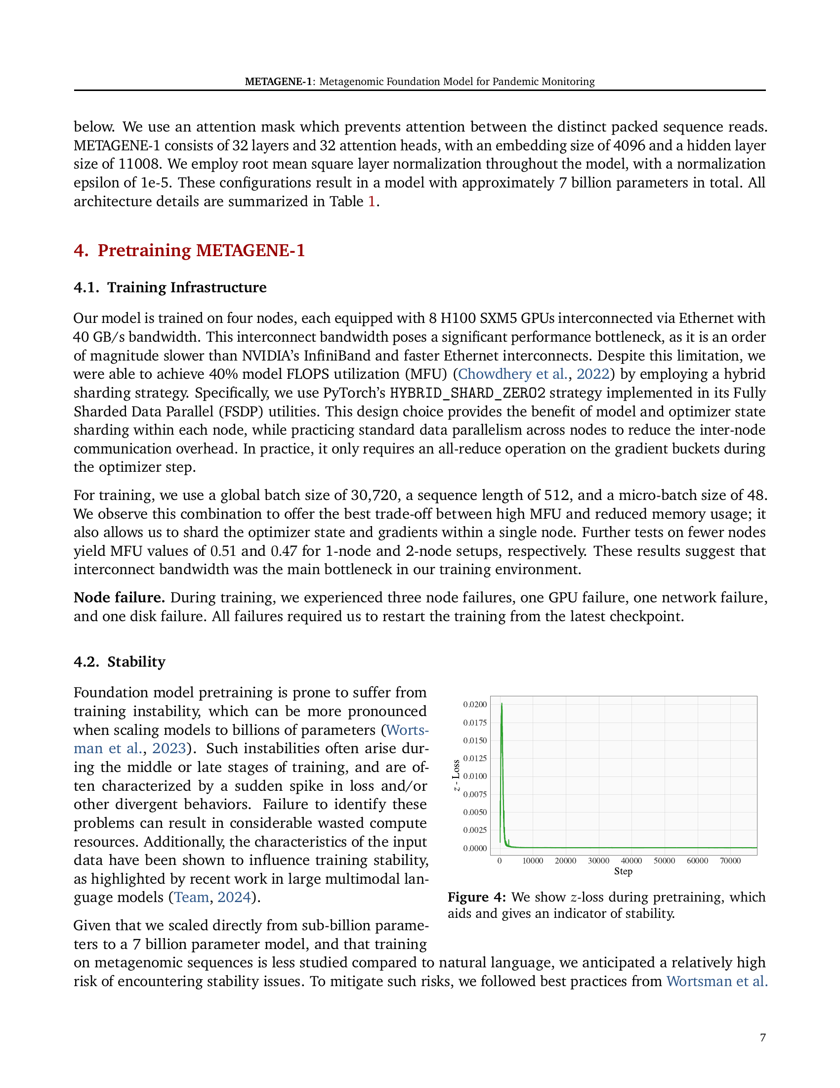
🔼 The figure shows a graph of the z-loss during the pretraining process of the METAGENE-1 model. The z-loss is a metric used to monitor the stability of the training process, and its behavior can indicate potential issues such as instability or divergence. A stable training process will typically show a smooth, gradually decreasing z-loss curve. Significant fluctuations or spikes in the z-loss can signal instability, which may require intervention to prevent the training from failing. The plot allows for visualization of the training stability of the model over time.
read the caption
Figure 4: We show z𝑧zitalic_z-loss during pretraining, which aids and gives an indicator of stability.

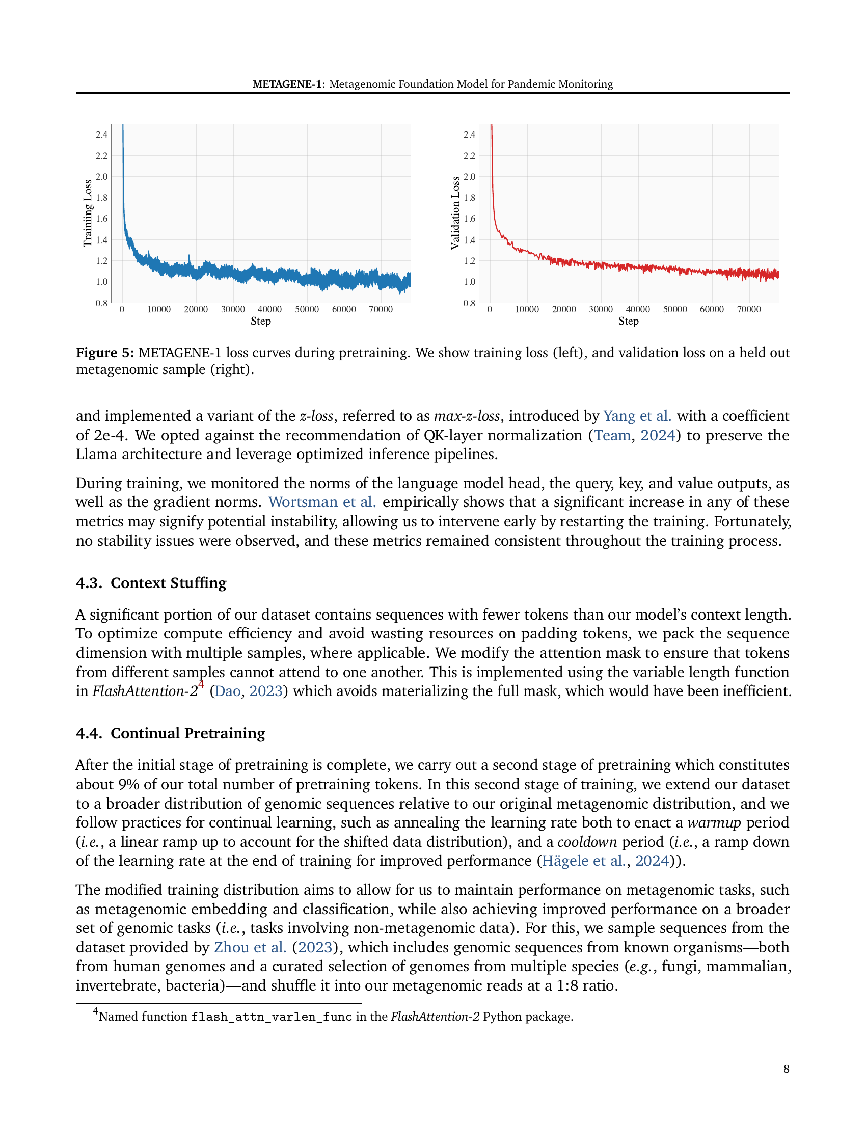
🔼 This figure displays the training and validation loss curves for the METAGENE-1 model during its pretraining phase. The left panel shows the training loss, which is the loss calculated on the training dataset during each iteration of training. The right panel shows the validation loss, which is the loss calculated on a separate held-out portion of the metagenomic dataset to assess the model’s generalization ability. The plots provide insights into the model’s learning progress and help identify potential issues such as overfitting (where the training loss decreases while validation loss increases). The slight oscillations visible in the training curve result from the pseudo-random data shuffling employed for training efficiency.
read the caption
Figure 5: METAGENE-1 loss curves during pretraining. We show training loss (left), and validation loss on a held out metagenomic sample (right).

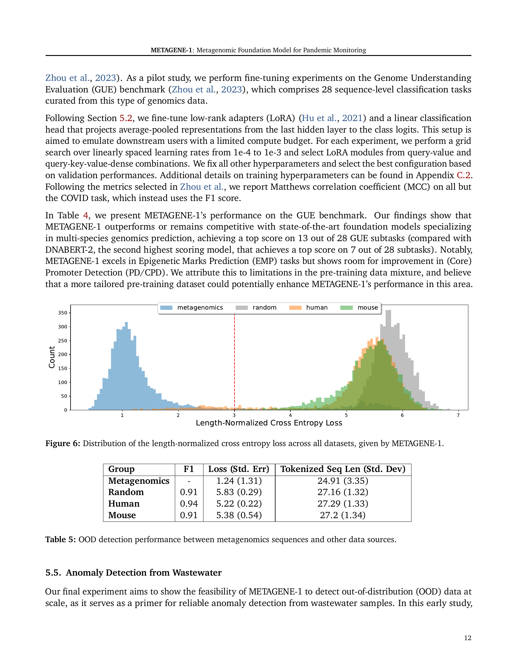
🔼 Figure 6 shows the distribution of length-normalized cross-entropy loss values generated by METAGENE-1 across four different datasets: metagenomics, random sequences, human genome sequences, and mouse genome sequences. The length normalization accounts for differences in sequence length between these datasets, making the comparisons more meaningful. The figure is a histogram showing the frequency distribution of these loss values for each dataset. This visualization helps illustrate the model’s ability to distinguish between in-distribution (metagenomics) and out-of-distribution (OOD) data, which is relevant for anomaly detection tasks.
read the caption
Figure 6: Distribution of the length-normalized cross entropy loss across all datasets, given by METAGENE-1.
More on tables
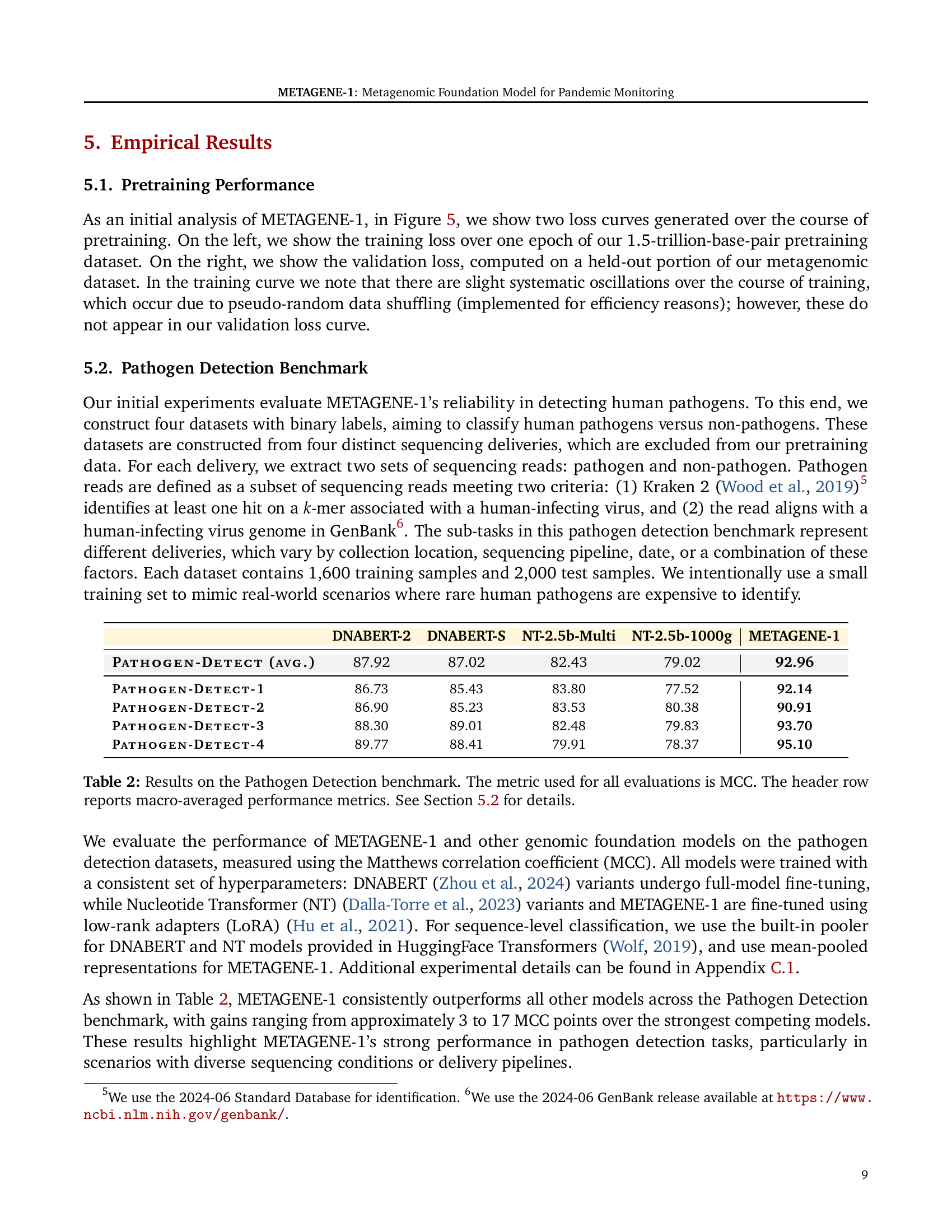
| DNABERT-2 | DNABERT-S | NT-2.5b-Multi | NT-2.5b-1000g | METAGENE-1 | |
|---|---|---|---|---|---|
| Pathogen-Detect (avg.) | 87.92 | 87.02 | 82.43 | 79.02 | 92.96 |
| Pathogen-Detect-1 | 86.73 | 85.43 | 83.80 | 77.52 | 92.14 |
| Pathogen-Detect-2 | 86.90 | 85.23 | 83.53 | 80.38 | 90.91 |
| Pathogen-Detect-3 | 88.30 | 89.01 | 82.48 | 79.83 | 93.70 |
| Pathogen-Detect-4 | 89.77 | 88.41 | 79.91 | 78.37 | 95.10 |
🔼 This table presents the results of the pathogen detection benchmark. Four different datasets (PATHOGEN-DETECT-1 through 4), each derived from separate wastewater sequencing deliveries and excluding data used for model pretraining, were used for evaluation. The model’s performance on each dataset is evaluated using the Matthews Correlation Coefficient (MCC), a measure commonly used for evaluating classification model performance. The header row displays the macro-averaged MCC across all four datasets, providing a single summary metric. Details on how these datasets were constructed and the specifics of the evaluation methodology are provided in Section 5.2 of the paper.
read the caption
Table 2: Results on the Pathogen Detection benchmark. The metric used for all evaluations is MCC. The header row reports macro-averaged performance metrics. See Section 5.2 for details.
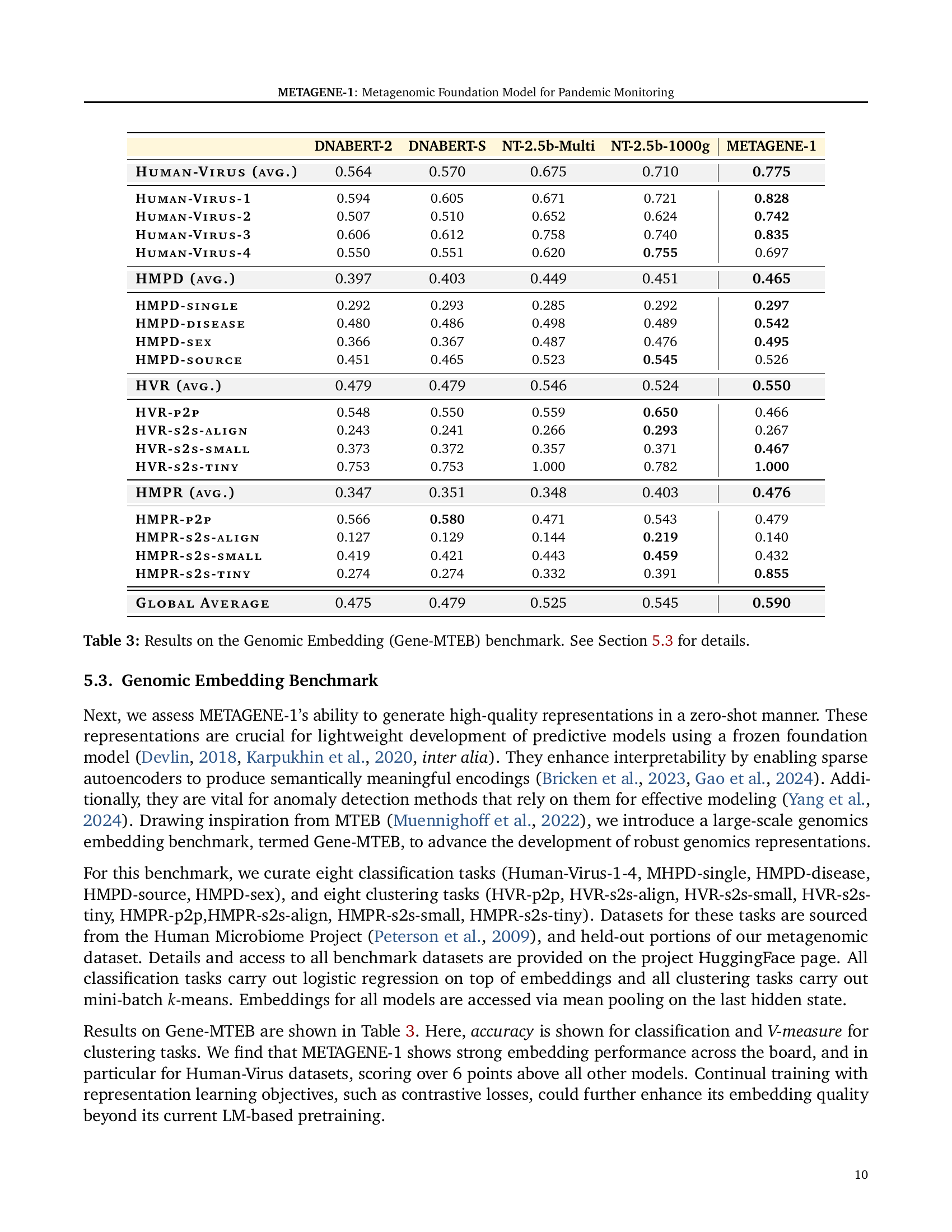
| DNABERT-2 | DNABERT-S | NT-2.5b-Multi | NT-2.5b-1000g | METAGENE-1 | |
|---|---|---|---|---|---|
| Human-Virus (avg.) | 0.564 | 0.570 | 0.675 | 0.710 | 0.775 |
| Human-Virus-1 | 0.594 | 0.605 | 0.671 | 0.721 | 0.828 |
| Human-Virus-2 | 0.507 | 0.510 | 0.652 | 0.624 | 0.742 |
| Human-Virus-3 | 0.606 | 0.612 | 0.758 | 0.740 | 0.835 |
| Human-Virus-4 | 0.550 | 0.551 | 0.620 | 0.755 | 0.697 |
| HMPD (avg.) | 0.397 | 0.403 | 0.449 | 0.451 | 0.465 |
| HMPD-single | 0.292 | 0.293 | 0.285 | 0.292 | 0.297 |
| HMPD-disease | 0.480 | 0.486 | 0.498 | 0.489 | 0.542 |
| HMPD-sex | 0.366 | 0.367 | 0.487 | 0.476 | 0.495 |
| HMPD-source | 0.451 | 0.465 | 0.523 | 0.545 | 0.526 |
| HVR (avg.) | 0.479 | 0.479 | 0.546 | 0.524 | 0.550 |
| HVR-p2p | 0.548 | 0.550 | 0.559 | 0.650 | 0.466 |
| HVR-s2s-align | 0.243 | 0.241 | 0.266 | 0.293 | 0.267 |
| HVR-s2s-small | 0.373 | 0.372 | 0.357 | 0.371 | 0.467 |
| HVR-s2s-tiny | 0.753 | 0.753 | 1.000 | 0.782 | 1.000 |
| HMPR (avg.) | 0.347 | 0.351 | 0.348 | 0.403 | 0.476 |
| HMPR-p2p | 0.566 | 0.580 | 0.471 | 0.543 | 0.479 |
| HMPR-s2s-align | 0.127 | 0.129 | 0.144 | 0.219 | 0.140 |
| HMPR-s2s-small | 0.419 | 0.421 | 0.443 | 0.459 | 0.432 |
| HMPR-s2s-tiny | 0.274 | 0.274 | 0.332 | 0.391 | 0.855 |
| Global Average | 0.475 | 0.479 | 0.525 | 0.545 | 0.590 |
🔼 Table 3 presents the results of the Gene-MTEB benchmark, a newly introduced evaluation metric designed to assess the quality of genomic sequence embeddings generated by various foundation models. It evaluates the models’ zero-shot performance on eight classification and eight clustering tasks using data from the Human Microbiome Project and a held-out portion of the METAGENE-1 metagenomic dataset. The table compares the performance of METAGENE-1 against several other state-of-the-art genomic models, specifically DNABERT-2, DNABERT-S, and two variants of Nucleotide Transformer (NT-2.5b-Multi and NT-2.5b-1000g). The results highlight METAGENE-1’s performance across different genomic tasks.
read the caption
Table 3: Results on the Genomic Embedding (Gene-MTEB) benchmark. See Section 5.3 for details.
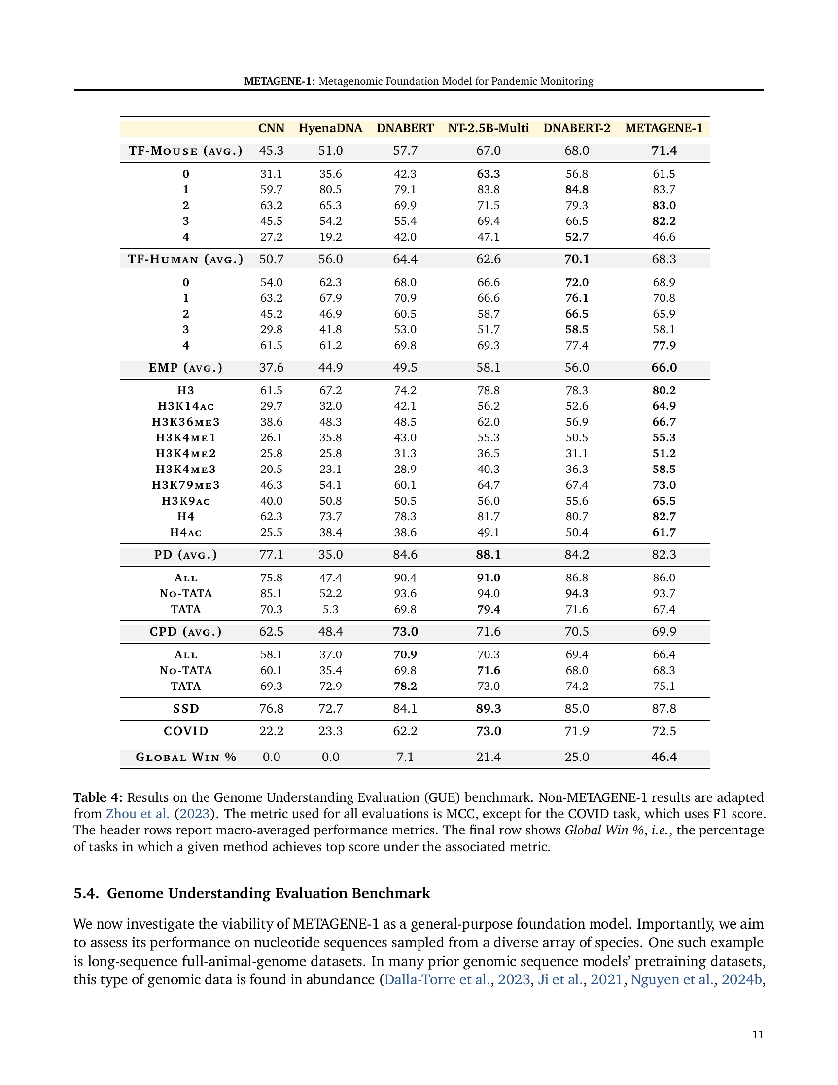
| CNN | HyenaDNA | DNABERT | NT-2.5B-Multi | DNABERT-2 | METAGENE-1 | |
|---|---|---|---|---|---|---|
| TF-Mouse (avg.) | 45.3 | 51.0 | 57.7 | 67.0 | 68.0 | 71.4 |
| 0 | 31.1 | 35.6 | 42.3 | 63.3 | 56.8 | 61.5 |
| 1 | 59.7 | 80.5 | 79.1 | 83.8 | 84.8 | 83.7 |
| 2 | 63.2 | 65.3 | 69.9 | 71.5 | 79.3 | 83.0 |
| 3 | 45.5 | 54.2 | 55.4 | 69.4 | 66.5 | 82.2 |
| 4 | 27.2 | 19.2 | 42.0 | 47.1 | 52.7 | 46.6 |
| TF-Human (avg.) | 50.7 | 56.0 | 64.4 | 62.6 | 70.1 | 68.3 |
| 0 | 54.0 | 62.3 | 68.0 | 66.6 | 72.0 | 68.9 |
| 1 | 63.2 | 67.9 | 70.9 | 66.6 | 76.1 | 70.8 |
| 2 | 45.2 | 46.9 | 60.5 | 58.7 | 66.5 | 65.9 |
| 3 | 29.8 | 41.8 | 53.0 | 51.7 | 58.5 | 58.1 |
| 4 | 61.5 | 61.2 | 69.8 | 69.3 | 77.4 | 77.9 |
| EMP (avg.) | 37.6 | 44.9 | 49.5 | 58.1 | 56.0 | 66.0 |
| H3 | 61.5 | 67.2 | 74.2 | 78.8 | 78.3 | 80.2 |
| H3K14ac | 29.7 | 32.0 | 42.1 | 56.2 | 52.6 | 64.9 |
| H3K36me3 | 38.6 | 48.3 | 48.5 | 62.0 | 56.9 | 66.7 |
| H3K4me1 | 26.1 | 35.8 | 43.0 | 55.3 | 50.5 | 55.3 |
| H3K4me2 | 25.8 | 25.8 | 31.3 | 36.5 | 31.1 | 51.2 |
| H3K4me3 | 20.5 | 23.1 | 28.9 | 40.3 | 36.3 | 58.5 |
| H3K79me3 | 46.3 | 54.1 | 60.1 | 64.7 | 67.4 | 73.0 |
| H3K9ac | 40.0 | 50.8 | 50.5 | 56.0 | 55.6 | 65.5 |
| H4 | 62.3 | 73.7 | 78.3 | 81.7 | 80.7 | 82.7 |
| H4ac | 25.5 | 38.4 | 38.6 | 49.1 | 50.4 | 61.7 |
| PD (avg.) | 77.1 | 35.0 | 84.6 | 88.1 | 84.2 | 82.3 |
| All | 75.8 | 47.4 | 90.4 | 91.0 | 86.8 | 86.0 |
| No-TATA | 85.1 | 52.2 | 93.6 | 94.0 | 94.3 | 93.7 |
| TATA | 70.3 | 5.3 | 69.8 | 79.4 | 71.6 | 67.4 |
| CPD (avg.) | 62.5 | 48.4 | 73.0 | 71.6 | 70.5 | 69.9 |
| All | 58.1 | 37.0 | 70.9 | 70.3 | 69.4 | 66.4 |
| No-TATA | 60.1 | 35.4 | 69.8 | 71.6 | 68.0 | 68.3 |
| TATA | 69.3 | 72.9 | 78.2 | 73.0 | 74.2 | 75.1 |
| SSD | 76.8 | 72.7 | 84.1 | 89.3 | 85.0 | 87.8 |
| COVID | 22.2 | 23.3 | 62.2 | 73.0 | 71.9 | 72.5 |
| Global Win % | 0.0 | 0.0 | 7.1 | 21.4 | 25.0 | 46.4 |
🔼 Table 4 presents the results of the Genome Understanding Evaluation (GUE) benchmark, comparing METAGENE-1’s performance against other state-of-the-art genomic foundation models. The GUE benchmark consists of 28 sequence-level classification tasks focused on various aspects of genomics. The primary evaluation metric is the Matthews Correlation Coefficient (MCC), except for the COVID-19 task which uses the F1 score. The table displays the MCC or F1 score for each model on each task and then shows the macro-averaged performance across all tasks. The final row shows the ‘Global Win %’, indicating the percentage of tasks where each model achieved the highest score. Results for models other than METAGENE-1 are taken from Zhou et al. (2023). This provides a comprehensive comparison of METAGENE-1’s performance across a broad range of genomic tasks.
read the caption
Table 4: Results on the Genome Understanding Evaluation (GUE) benchmark. Non-METAGENE-1 results are adapted from Zhou et al. (2023). The metric used for all evaluations is MCC, except for the COVID task, which uses F1 score. The header rows report macro-averaged performance metrics. The final row shows Global Win %, i.e., the percentage of tasks in which a given method achieves top score under the associated metric.
| Group | F1 | Loss (Std. Err) | Tokenized Seq Len (Std. Dev) |
|---|---|---|---|
| Metagenomics | - | 1.24 (1.31) | 24.91 (3.35) |
| Random | 0.91 | 5.83 (0.29) | 27.16 (1.32) |
| Human | 0.94 | 5.22 (0.22) | 27.29 (1.33) |
| Mouse | 0.91 | 5.38 (0.54) | 27.2 (1.34) |
🔼 This table presents the out-of-distribution (OOD) detection performance of the METAGENE-1 model. It compares the model’s ability to distinguish metagenomic sequences from other data sources, including randomly generated sequences and sequences from human and mouse genomes. The evaluation metric used is F1 score, and the table shows the F1 scores and standard errors for each data source, along with the average sequence length for each data source. The results demonstrate METAGENE-1’s effectiveness in identifying metagenomic sequences as in-distribution data and other types of sequences as out-of-distribution data.
read the caption
Table 5: OOD detection performance between metagenomics sequences and other data sources.
| Model | Setting |
|---|---|
| DNABERT-⋆ | Full Model |
| NT-⋆ | LoRA |
| METAGENE-1 | LoRA |
| LoRA Modules | query, key, value, dense |
| LoRA Rank | 8 |
| LoRA α | 16 |
| LoRA Dropout | 0.1 |
| Optimizer | AdamW |
| Optimizer Momentum | β1, β2 = 0.9, 0.999 |
| Learning Rate | 1e-4Λ |
| LR Scheduler | Linear Warmup + Constant LR |
| Warmup Steps | 50 |
| Weight Decay | 0.01 |
| Denominator ϵ | 1e-8 |
| Precision | BF16-mixed |
| Batch Size | 32 |
| Epochs | 10 |
| Hardware | NVIDIA A100 80GB |
🔼 This table details the hyperparameters used for fine-tuning various models on the pathogen detection task. It lists the model (DNABERT-2, DNABERT-S, Nucleotide Transformer variants, and METAGENE-1), the type of fine-tuning (full model or LoRA), the LoRA modules used (if applicable), LoRA rank, alpha, and dropout rate. Optimizer parameters (optimizer, momentum, learning rate, learning rate scheduler, warmup steps, weight decay, denominator epsilon), precision, batch size, and number of epochs are also provided. A note indicates that for DNABERT-S, the learning rate was halved due to observed oscillations in training loss.
read the caption
Table 6: Hyperparameter settings for the Pathogen Detection fine-tuning experiments. ΛΛ\Lambdaroman_Λ: for DNABERT-S, we halve the learning to 5e-5 as we observe clear oscillation behavior in the training loss.
| LoRA Modules | query, key, value, denseΛ |
|---|---|
| LoRA Rank | 8 |
| LoRA α | 16 |
| LoRA Dropout | 0.1 |
| Optimizer | AdamW |
| Optimizer Momentum (β1, β2) | 0.9, 0.999 |
| Learning Rate | {1e-4⋯1e-3}Ω |
| LR Scheduler | Linear Warmup + Constant LR |
| Warmup Steps | 50 |
| Weight Decay | 0.01 |
| Denominator ϵ | 1e-8 |
| Precision | BF16-mixed |
| Batch Size | 32 |
| Epochs | 10 |
| Hardware | NVIDIA A100 80GB |
🔼 Table 7 details the hyperparameters used during fine-tuning experiments for the Genome Understanding Evaluation (GUE) benchmark. It specifies that Low-Rank Adaptation (LoRA) was applied to either query-value or query-key-value-dense modules, with a rank of 8 and alpha of 16. A dropout rate of 0.1 was used. The AdamW optimizer was employed with a learning rate tuned across an equally-spaced grid from 1e-4 to 1e-3, along with other standard hyperparameter settings. All hyperparameters were selected based on their performance on validation sets.
read the caption
Table 7: Hyperparameter settings for the GUE fine-tuning experiments. ΛΛ\Lambdaroman_Λ: LoRA is applied to query-value or query-key-value-dense modules. ΩΩ\Omegaroman_Ω: learning rates are tuned over a equally-spaced grid of 1e-4, 2e-4, ⋯⋯\cdots⋯, 1e-3. All hyperparameters are selected according to performances on validation sets.
Full paper#
