↗ arXiv ↗ Hugging Face ↗ Papers with Code
TL;DR#
Current instruction tuning for code LLMs relies on limited code snippets, hindering the generation of diverse and complex data. This restricts the models’ ability to handle real-world tasks. EpiCoder tackles this problem by introducing a novel feature tree-based framework. This framework models semantic relationships between code elements, enabling the generation of nuanced data. By carefully controlling the depth and breadth of the feature trees, EpiCoder can generate code of varying complexities.
EpiCoder demonstrates state-of-the-art performance on multiple benchmarks. This highlights the effectiveness of the proposed data synthesis method. The rigorous evaluation and detailed analysis of data complexity and diversity, using both software engineering principles and an LLM-as-a-judge method, further validate the approach’s merits. EpiCoder shows great potential for scaling to repository-level code data synthesis, a significant step forward in the field.
Key Takeaways#
Why does it matter?#
This paper is crucial for researchers in code generation and large language models because it introduces a novel approach to data synthesis that significantly improves the quality and diversity of training data. This leads to better-performing models capable of handling more complex tasks, and opens up new avenues for research into large-scale code generation. The rigorous evaluation and analysis presented provide valuable insights for future work in this area.
Visual Insights#

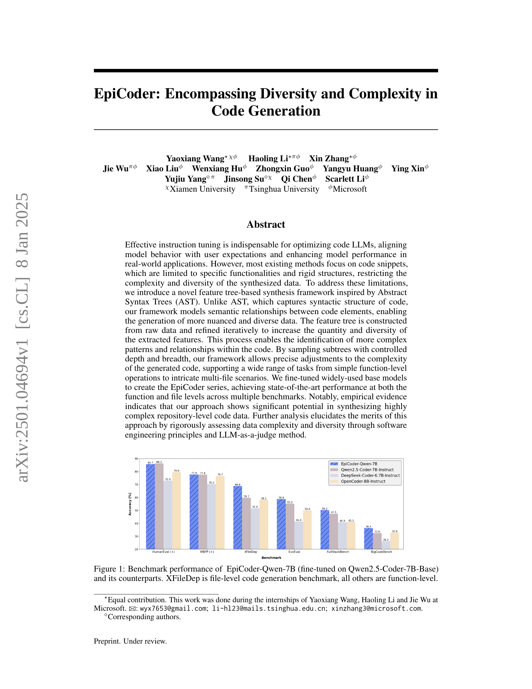
🔼 Figure 1 presents a comparison of the performance of EpiCoder-Qwen-7B (a model fine-tuned using the Qwen2.5-Coder-7B-Base model) against several other code generation models across various benchmarks. The benchmarks assess code generation capabilities at both the function level (where the model generates code for single functions) and the file level (where the model generates multiple files and handles dependencies between them). XFileDep is a benchmark specifically designed for file-level code generation, while the other benchmarks evaluate function-level code generation performance. The figure displays the accuracy of each model on each benchmark, allowing for a direct comparison of their relative strengths and weaknesses in various code generation tasks.
read the caption
Figure 1: Benchmark performance of EpiCoder-Qwen-7B (fine-tuned on Qwen2.5-Coder-7B-Base) and its counterparts. XFileDep is file-level code generation benchmark, all others are function-level.
| Model | Base Model | HumanEval Base | HumanEval Plus | MBPP Base | MBPP Plus | Average |
|---|---|---|---|---|---|---|
| GPT-4-Turbo (April 2024) | - | 90.2 | 86.6 | 85.7 | 73.3 | 84.0 |
| GPT-4 (May 2023) | - | 88.4 | 79.3 | - | - | - |
| GPT-3.5-Turbo (Nov 2023) | - | 76.8 | 70.7 | 82.5 | 69.7 | 75.0 |
| claude-3-opus (Mar 2024) | - | 82.9 | 77.4 | 89.4 | 73.3 | 80.8 |
| claude-3-sonnet (Mar 2024) | - | 70.7 | 64.0 | 83.6 | 69.3 | 71.9 |
| claude-3-haiku (Mar 2024) | - | 76.8 | 68.9 | 80.2 | 68.8 | 73.7 |
| Qwen2.5-Coder-32B-Instruct | - | 92.1 | 87.2 | 90.5 | 77.0 | 86.7 |
| DeepSeek-Coder-V2-Instruct | - | 85.4 | 82.3 | 89.4 | 75.1 | 83.1 |
| OpenCoder-8B-Instruct | - | 81.7 | 77.4 | 82.0 | 71.4 | 78.1 |
| DeepSeek-Coder-33B-instruct | - | 81.1 | 75.0 | 80.4 | 70.1 | 76.7 |
| Codestral-22B-v0.1 | - | 79.9 | 73.8 | 72.5 | 61.9 | 72.0 |
| ~ 7B Scale | ||||||
| DSCoder-6.7B-Base | - | 47.6 | 39.6 | 72.0 | 58.7 | 54.5 |
| DeepSeekCoder-6.7b-Instruct | https://arxiv.org/html/2501.04694/figure/deepseek.png | 74.4 | 71.3 | 74.9 | 65.6 | 71.6 |
| Magicoder-S-DS | https://arxiv.org/html/2501.04694/figure/deepseek.png | 76.8 | 71.3 | 79.4 | 69.0 | 74.1 |
| WaveCoder-Ultra-6.7B | https://arxiv.org/html/2501.04694/figure/deepseek.png | 75.0 | 69.5 | 74.9 | 63.5 | 70.7 |
| OpenCodeInterpreter-DS-6.7B | https://arxiv.org/html/2501.04694/figure/deepseek.png | 77.4 | 72.0 | 76.5 | 66.4 | 73.1 |
| EpiCoder-DS-6.7B | https://arxiv.org/html/2501.04694/figure/deepseek.png | 80.5 | 76.8 | 81.5 | 68.3 | 76.8 |
| Qwen2.5-Coder-7B-Base | https://arxiv.org/html/2501.04694/figure/qwen2.png | 61.6 | 53.0 | 76.9 | 62.9 | 63.6 |
| Qwen2.5-Coder-7B-Instruct | https://arxiv.org/html/2501.04694/figure/qwen2.png | 88.4 | 84.1 | 83.5 | 71.7 | 81.9 |
| EpiCoder-Qwen-7B | https://arxiv.org/html/2501.04694/figure/qwen2.png | 89.0 | 82.3 | 84.1 | 71.4 | 81.7 |
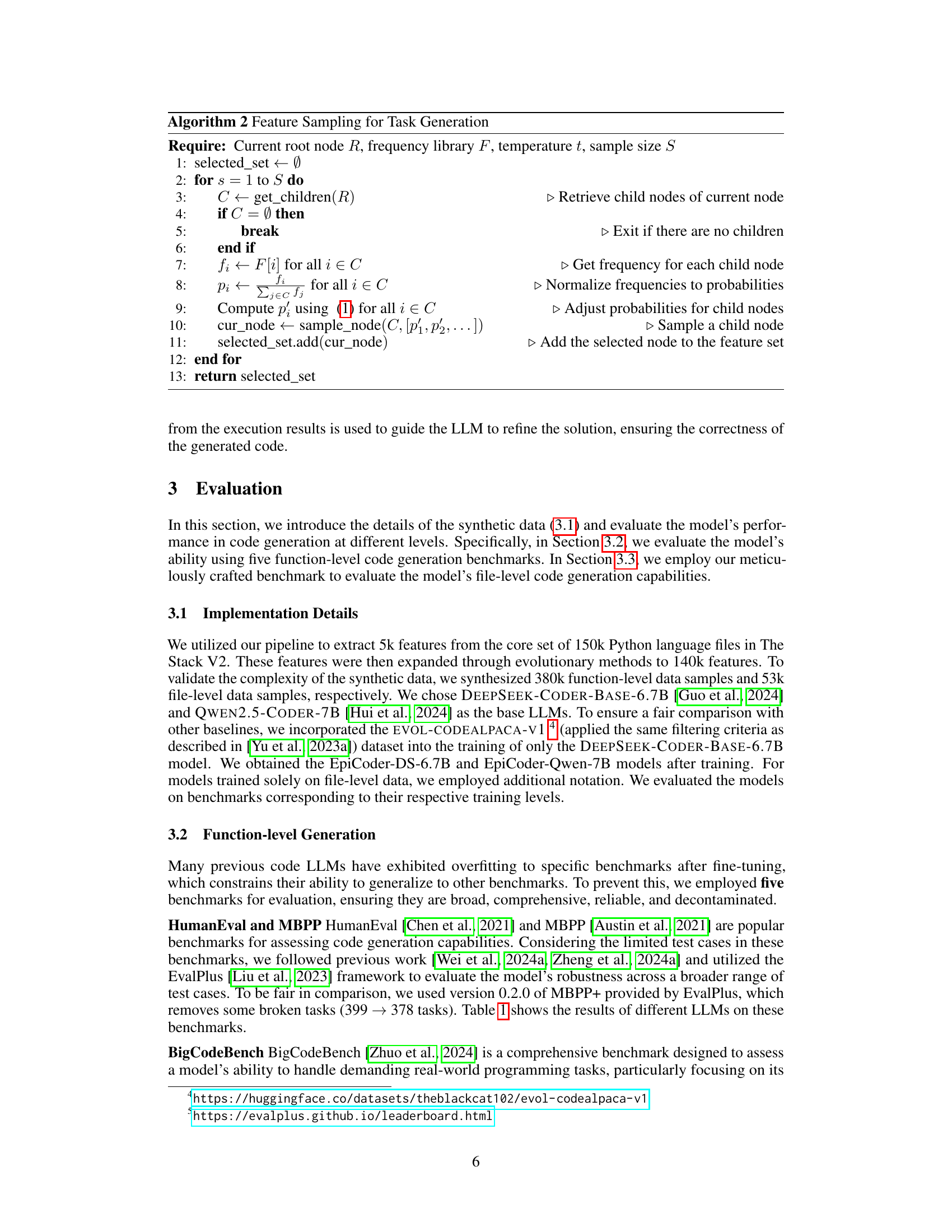
🔼 This table presents the pass@1 scores, a metric representing the percentage of correctly solved problems, achieved by various Large Language Models (LLMs) on two widely used code generation benchmarks: HumanEval and MBPP. The results are obtained using greedy decoding, a method of generating text. The ‘+’ symbol indicates an enhanced version of the benchmarks, likely including additional test cases or improved evaluation processes. The data is compiled from the EvalPlus Leaderboard, ensuring consistency and comparability across different LLMs.
read the caption
Table 1: Pass@1 (%) results of different LLMs on HumanEval (+) and MBPP (+) computed with greedy decoding. We report the results uniformly from the EvalPlus Leaderboard 444https://evalplus.github.io/leaderboard.html.
In-depth insights#
Feature Tree Synthesis#
Feature Tree Synthesis presents a novel approach to data generation for code LLMs, moving beyond the limitations of using simple code snippets. By constructing a tree-like structure that models semantic relationships between code elements, rather than just syntactic structures, it enables the generation of more nuanced and diverse data. This hierarchical representation allows for controllable complexity, enabling the creation of code ranging from simple operations to complex, multi-file scenarios. The iterative refinement of the feature tree, through both breadth and depth expansion, ensures that the synthesized data is both comprehensive and diverse, overcoming the inherent limitations of simpler methods. This method’s strength lies in its capacity to capture complex relationships within code and generate data that is far more representative of real-world software, leading to significant performance gains in code generation tasks. The ability to sample subtrees with controlled depth and breadth provides a mechanism to finely tune the complexity of the generated code, making it suitable for a wide range of applications and improving the robustness and generalizability of the trained model.
Code Data Complexity#
Analyzing code data complexity is crucial for evaluating the effectiveness of code generation models. Higher complexity datasets generally lead to models that generalize better and handle more diverse real-world programming scenarios. However, simply increasing code length or using more complex language features is insufficient; true complexity arises from intricate interactions between different code elements and modules. This involves considering multiple aspects: control flow (loops, branching, functions calls), data structures (use of lists, trees, graphs), and overall program architecture (modularity, coupling). A comprehensive analysis necessitates employing multiple metrics like Halstead complexity, cyclomatic complexity, and even leveraging LLMs to judge the overall complexity from a more holistic perspective. The choice of complexity metric should be aligned with the specific aspects of code generation being studied and the capabilities being targeted for the generated code. Data leakage is a significant concern, as models may overfit to specific characteristics in the training data instead of developing general abilities. Therefore, rigorous assessment techniques and well-designed evaluation benchmarks are essential to ensure that claims of superior model performance are indeed grounded in genuine improvements in generalizability, and not just an artifact of training data selection or overfitting.
Instruction Data Diversity#
Instruction data diversity is crucial for training robust and generalizable code large language models (LLMs). A diverse dataset ensures the model encounters a wide range of programming styles, complexities, and problem types, preventing overfitting to specific patterns in the training data. Without diversity, the model may perform exceptionally well on the training data but poorly generalize to unseen tasks. This is especially important for instruction-tuned LLMs, where the model is trained on instructions and corresponding code. The quality of instructions and their diversity in terms of problem complexity, coding style, and domain significantly impacts the resulting model’s capabilities. Therefore, generating diverse and high-quality instruction data is essential to advance the field of code generation and improve LLM performance.
Repo-Level CodeGen#
Repo-level code generation (CodeGen) signifies a significant advancement in AI-powered code synthesis, moving beyond the limitations of function- or file-level generation. This approach aims to generate entire software repositories, complete with multiple interconnected files, dependencies, and a well-defined project structure. The key challenge lies in handling the complexity inherent in large-scale codebases, including intricate relationships between modules, efficient resource management, and robust error handling. Successful repo-level CodeGen would revolutionize software development, enabling automated generation of complete, functional projects from high-level specifications. However, this also introduces new complexities in terms of data synthesis, model training, and evaluation. Generating realistic and diverse repository-level data for training is crucial, as this data would need to capture the multifaceted aspects of real-world projects. Furthermore, evaluating the quality and correctness of the generated repositories presents a significant challenge, requiring sophisticated metrics that go beyond simple functional testing. The potential benefits are enormous, including accelerated development cycles, improved code quality, and the ability to automate complex software engineering tasks. Despite challenges, repo-level CodeGen represents a fascinating and important research frontier with the potential to reshape software engineering.
LLM-as-Judge Method#
The concept of an “LLM-as-Judge Method” presents a novel approach to evaluating the quality of synthetic data generated for training LLMs. Instead of relying solely on traditional metrics, this method leverages the capabilities of a large language model to assess several qualitative aspects of the data, such as complexity, diversity, and the presence of biases. This is achieved by prompting the judge LLM with code samples and instructions to evaluate, effectively using the LLM’s understanding of programming principles and code style to provide a more nuanced assessment than traditional metrics could achieve. This approach offers significant advantages. Firstly, it directly addresses the limitations of quantitative metrics in capturing the subtleties of code quality. Secondly, it can assess a wider range of aspects that are essential for data quality, such as the overall code style, readability, efficiency, correctness, and robustness. Thirdly, it allows for easier adaptation to evolving coding practices and styles as the judge LLM can be readily updated. However, there are also challenges. There is the risk of bias in the judge LLM itself, which might influence its assessment. Additionally, the computational cost associated with such an approach may be considerably higher than traditional methods, and careful consideration is necessary to ensure that the judge LLM is well-suited for the specific tasks and data types being assessed. Nonetheless, this approach could be a valuable addition to the synthetic data evaluation process, particularly when the goal is to generate high-quality, diverse, and representative data for training state-of-the-art LLMs.
More visual insights#
More on figures

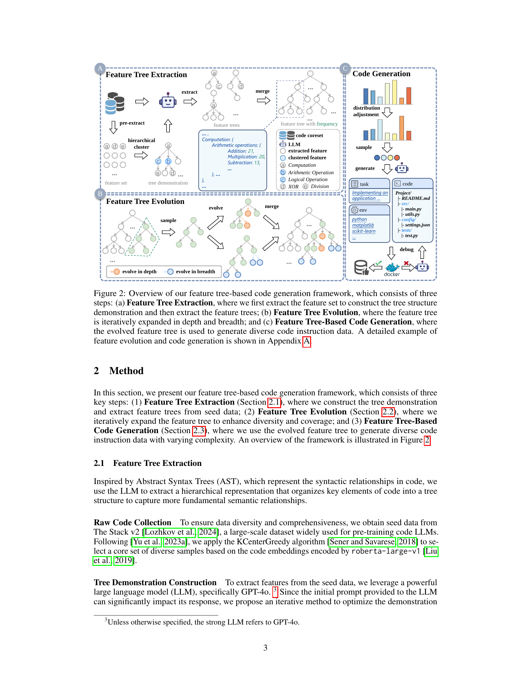
🔼 This figure illustrates the three main steps of the EpiCoder code generation framework: 1) Feature Tree Extraction: a feature set is extracted from raw code data to construct a tree structure demonstration, which then guides the extraction of feature trees that represent semantic relationships between code elements. 2) Feature Tree Evolution: the feature tree is iteratively expanded in both depth and breadth to enhance the diversity and quantity of extracted features. 3) Feature Tree-Based Code Generation: subtrees are sampled from the evolved feature tree to generate diverse code instruction data with varying complexity. Appendix A provides a detailed example of feature evolution and code generation.
read the caption
Figure 2: Overview of our feature tree-based code generation framework, which consists of three steps: (a) Feature Tree Extraction, where we first extract the feature set to construct the tree structure demonstration and then extract the feature trees; (b) Feature Tree Evolution, where the feature tree is iteratively expanded in depth and breadth; and (c) Feature Tree-Based Code Generation, where the evolved feature tree is used to generate diverse code instruction data. A detailed example of feature evolution and code generation is shown in Appendix A.
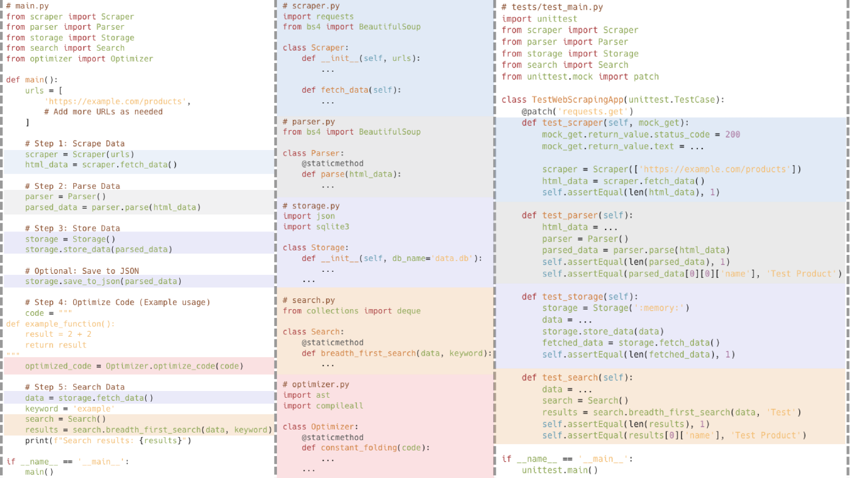
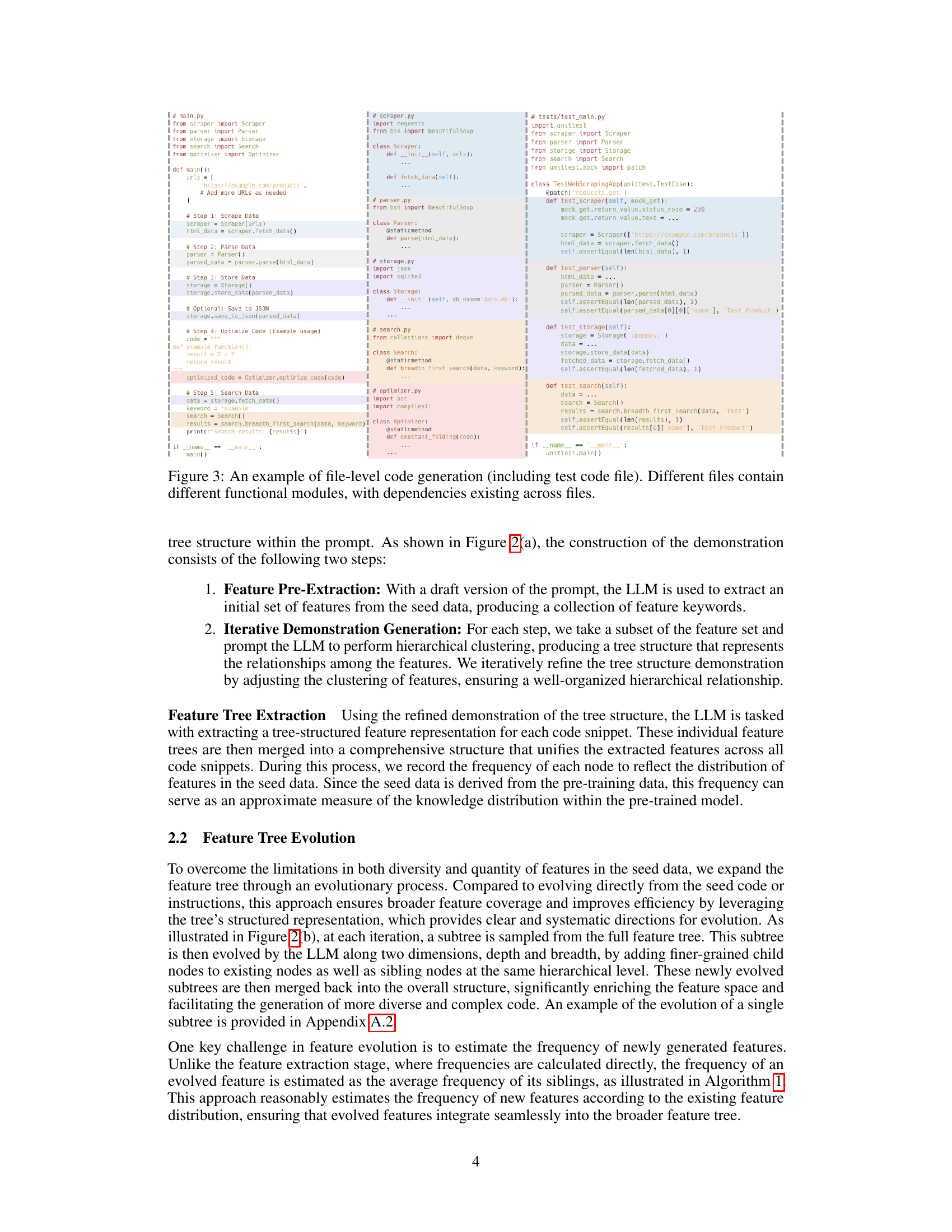
🔼 This figure showcases an example of file-level code generation, demonstrating the framework’s ability to produce more complex and realistic code. The example includes multiple files, each responsible for a distinct functional module (e.g., scraper, parser, storage, search, optimizer), and illustrates how these modules interact with each other. The dependencies between these modules highlight the ability of the framework to handle intricate multi-file projects, a capability that surpasses the limitations of simpler, single-file code generation methods.
read the caption
Figure 3: An example of file-level code generation (including test code file). Different files contain different functional modules, with dependencies existing across files.

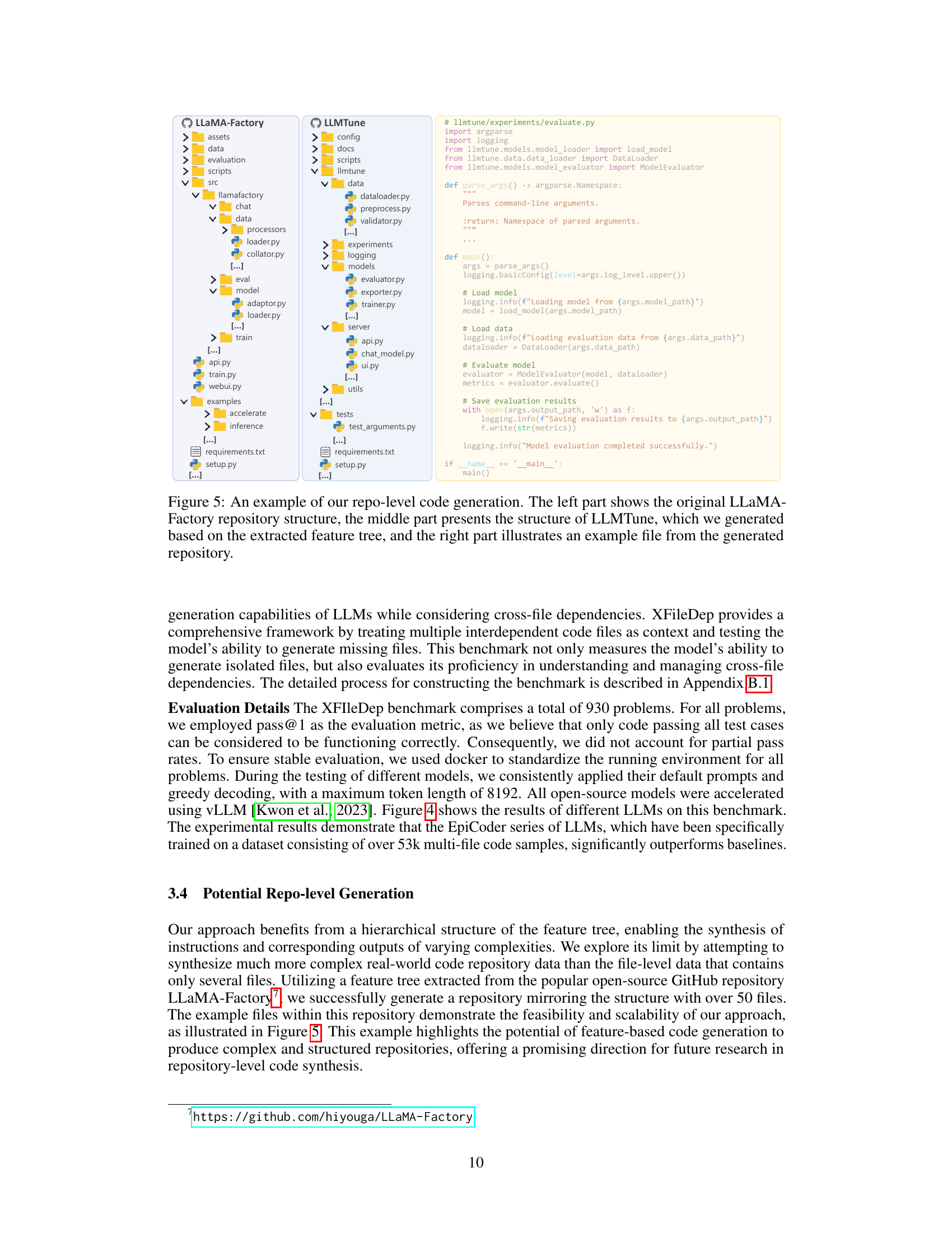
🔼 This figure displays the performance of various Large Language Models (LLMs) on the XFileDep benchmark, a specialized evaluation metric designed to assess the ability of LLMs to generate code that handles cross-file dependencies. The XFileDep benchmark goes beyond simpler function-level evaluations by testing the models’ understanding of the interrelationships between multiple files within a project. The chart visually compares the Pass@1 scores (the percentage of times the LLM correctly generated the needed code on the first attempt) for each model, illustrating their relative strengths in handling complex, multi-file code generation tasks using greedy decoding.
read the caption
Figure 4: Pass@1 (%) results of different LLMs on XFileDep computed with greedy decoding.

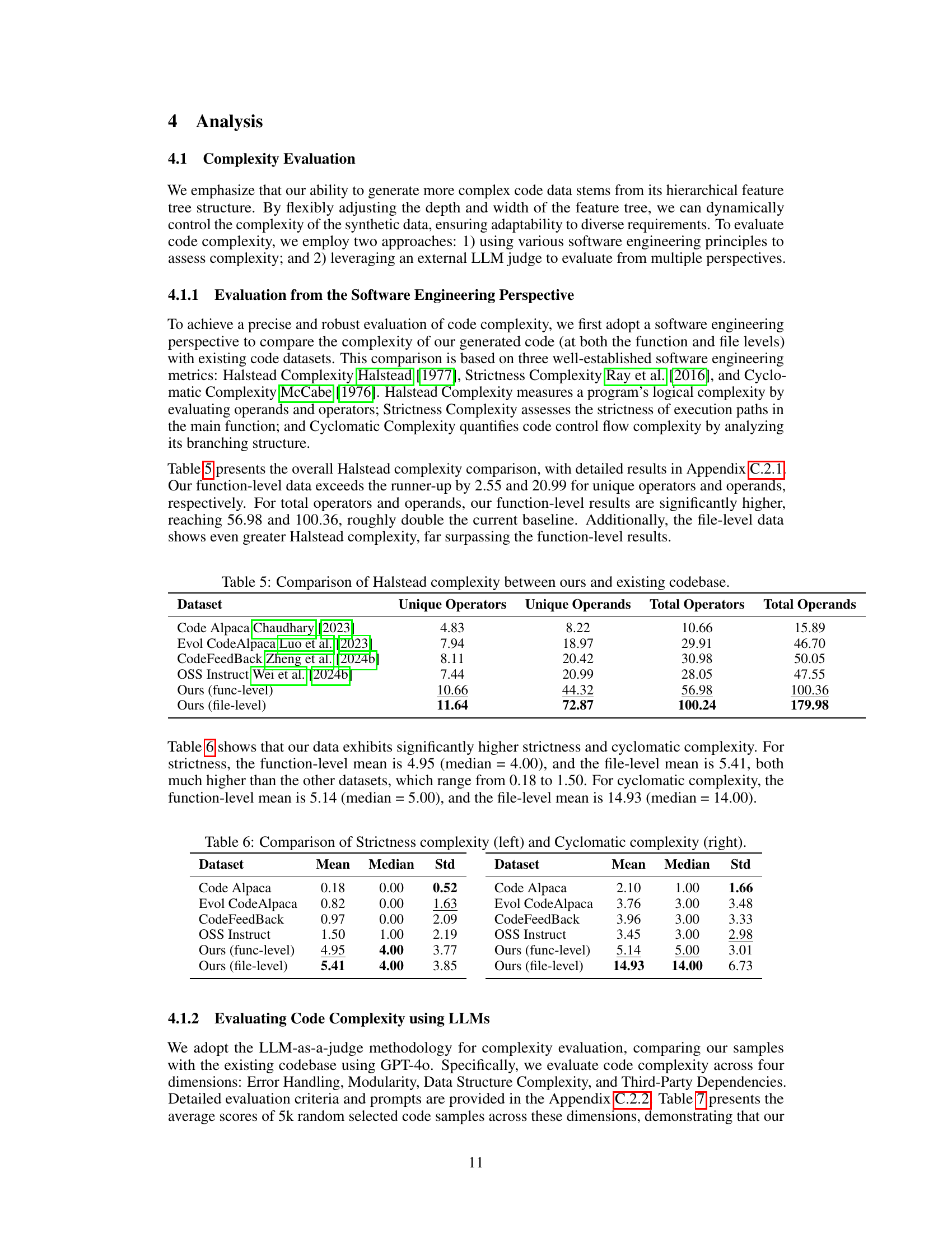
🔼 Figure 5 showcases the EpiCoder model’s capability for repository-level code generation. The figure is a three-panel comparison. The left panel displays the original file structure of the LLaMA-Factory repository. The middle panel shows the structure of the LLMTune repository, which was generated by EpiCoder using its feature tree-based approach. The right panel provides a sample code file from this newly generated LLMTune repository to illustrate the synthesized code’s characteristics. This demonstrates EpiCoder’s ability to generate code that mimics real-world repository structures and complexity.
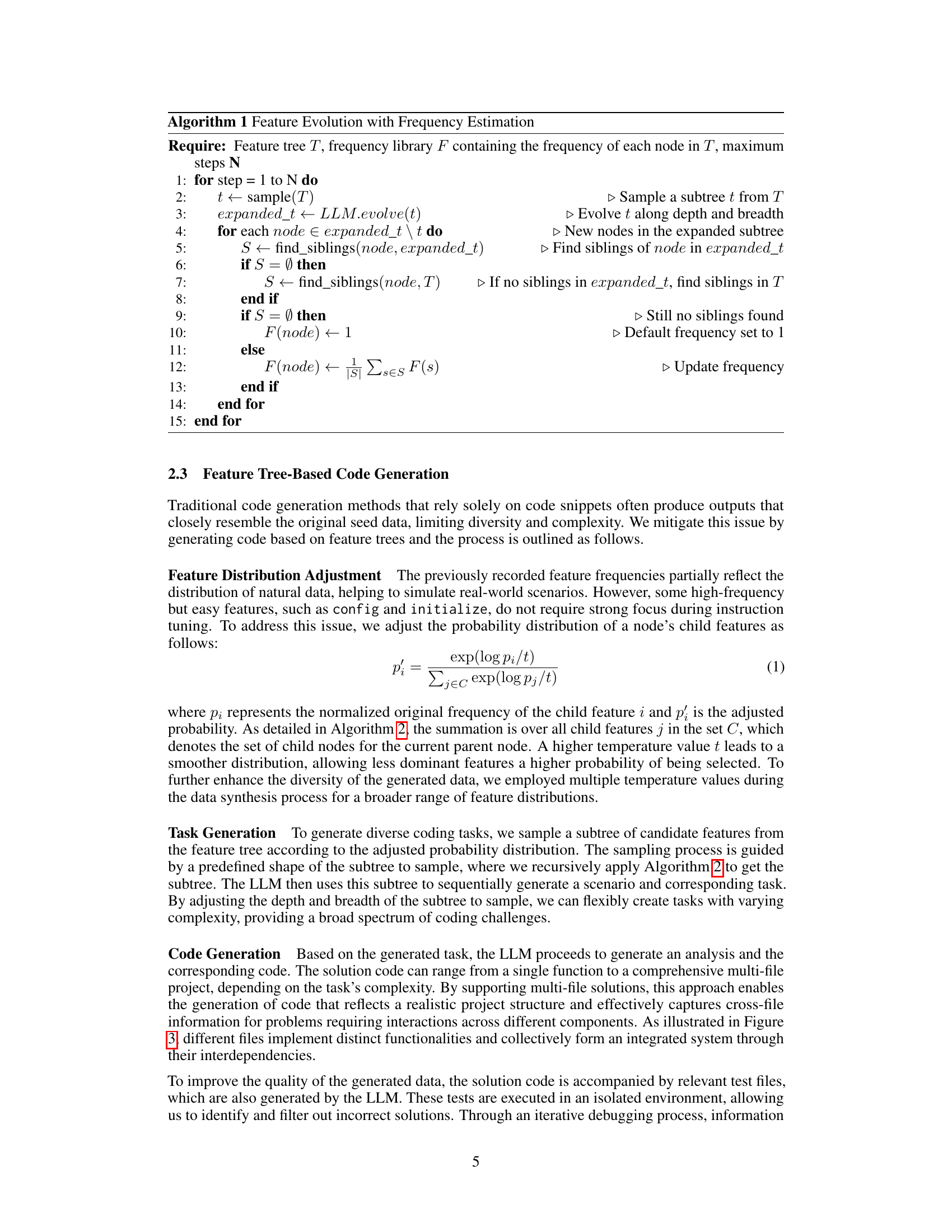
read the caption
Figure 5: An example of our repo-level code generation. The left part shows the original LLaMA-Factory repository structure, the middle part presents the structure of LLMTune, which we generated based on the extracted feature tree, and the right part illustrates an example file from the generated repository.

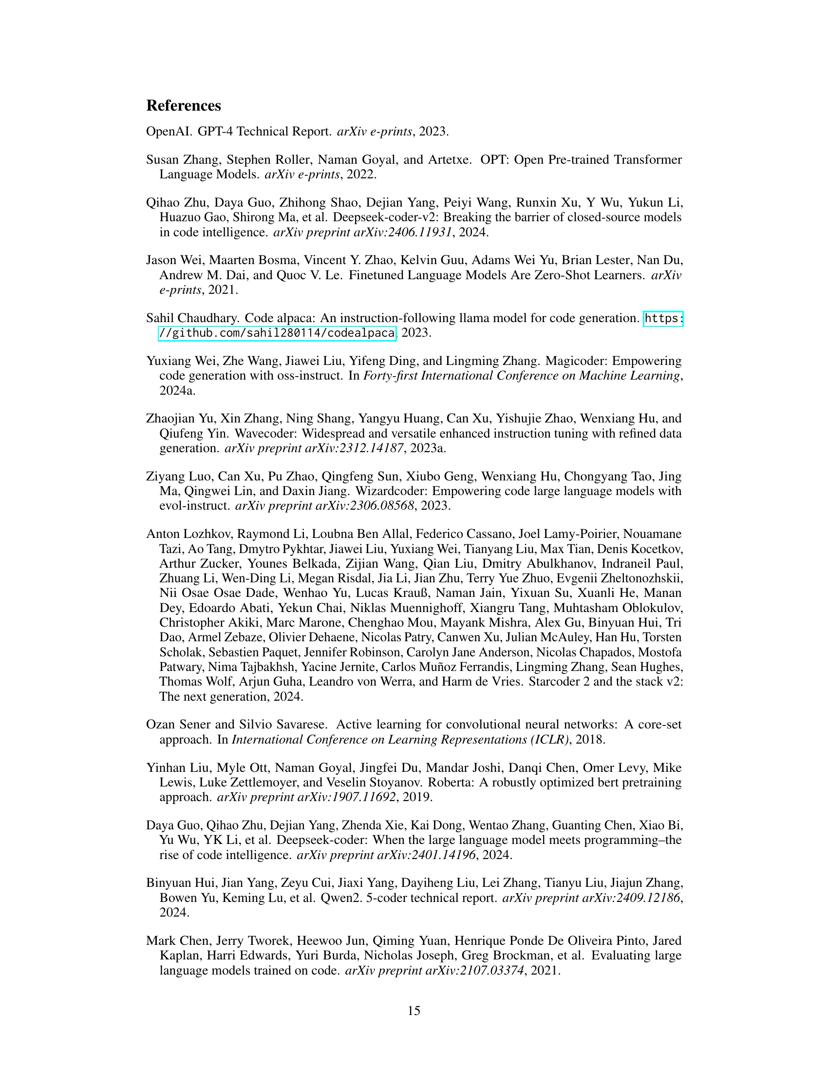
🔼 This figure displays the cosine similarity scores between the embeddings of various code datasets (including the authors’ own datasets and other existing datasets) and three popular code generation benchmarks: HumanEval, MBPP, and BigCodeBench. The distribution of these scores helps to visualize the degree of similarity between the training data and the benchmark datasets, providing insights into the potential for data leakage or overfitting. A high degree of similarity between a training dataset and a benchmark suggests potential overfitting.
read the caption
Figure 6: The distribution of cosine similarity scores between different various datasets and the benchmark datasets HumanEval, MBPP, and BigCodeBench.

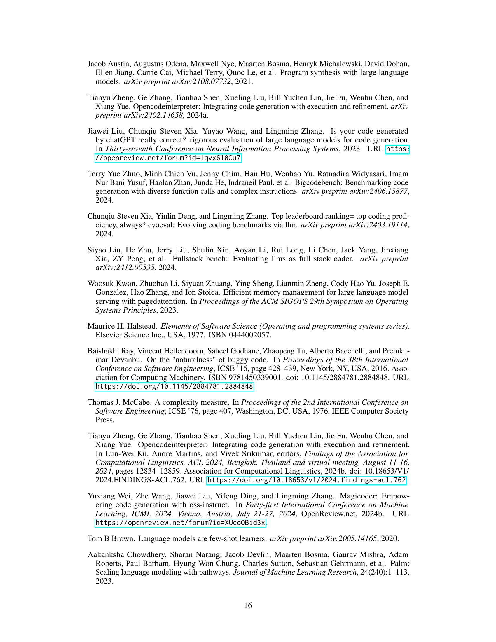
🔼 This figure presents the scaling law observed in code instruction data. It demonstrates how model performance, measured by Pass@1 accuracy on three widely-used benchmarks (HumanEval, MBPP, and BigCodeBench), improves as the size of the training dataset increases. Data points were randomly sampled from a total of 380,000 data points to illustrate the relationship between dataset size and model accuracy. The graph shows that performance continues to improve even at larger dataset sizes, suggesting the data’s diversity prevents overfitting.
read the caption
Figure 7: The scaling law of code instruction data. The results obtained from randomly sampled subsets of 380k data points across the HumanEval, MBPP, and BigCodeBench benchmarks.

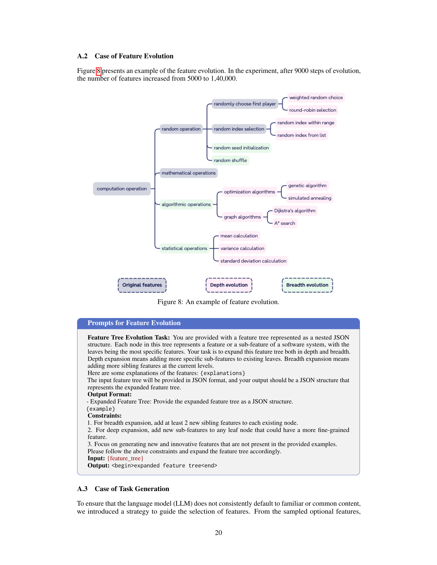
🔼 This figure illustrates the process of feature tree evolution in the EpiCoder code generation framework. Starting with an initial set of 5000 features, the tree is iteratively expanded both in depth (adding more specific sub-features to existing features) and breadth (adding new sibling features at the same level). After 9000 steps of evolution, the number of features increases significantly to 140,000. The figure visually represents this growth using a tree-like structure, showing how the initial features branch out and evolve into a much larger and more diverse set of features suitable for generating diverse and complex code instructions.
read the caption
Figure 8: An example of feature evolution.

🔼 This Sankey diagram illustrates the process of constructing the XFileDep benchmark dataset. It starts with 35,000 initial cross-file data samples. After filtering for samples with at least 5 files and sufficient complexity, 2,934 samples remain. Further filtering based on runtime and test requirements results in 2,231 samples. Test case augmentation expands this to 611 samples that pass the tests. Finally, after iterative test refinement and unsafe filtering steps, 930 samples form the final XFileDep dataset.
read the caption
Figure 9: The Sankey diagram for the creation of the XFileDep benchmark, with numbers indicating the quantity of data samples.

🔼 This figure shows two histograms. The left histogram displays the distribution of the number of files in each data sample used for the XFileDep benchmark after filtering, showing the prevalence of samples with varying numbers of files. The right histogram illustrates the distribution of the average file length (in characters) within each sample, providing insight into the size and complexity of the code files.
read the caption
Figure 10: the distribution of file quantities and the average file length for each data sample.

🔼 This figure displays pairs of code snippets, one from the HumanEval benchmark dataset and the other from the evol-codealpaca-v1 dataset. These pairs are selected based on their cosine similarity scores, calculated using embeddings generated from the ‘output’ sections of the training dataset and the ‘prompt + canonical_solution’ of the HumanEval dataset. The figure visually represents how similar the code generated by the evol-codealpaca-v1 model is to the canonical solutions in the HumanEval dataset, indicating potential data leakage issues. The varying similarity scores highlight the degrees of overlap between the datasets.
read the caption
Figure 11: Cases from the HumanEval benchmark dataset (left) and the evol-codealpaca-v1 dataset (right) with varying similarity. The embeddings are computed based on the 'output' portions of the training dataset and the 'prompt + canonical_solution' of the HumanEval benchmark data.
More on tables
| Model | Base | BigCodeBench-Full Complete | BigCodeBench-Full Instruct | BigCodeBench-Hard Complete | BigCodeBench-Hard Instruct | Avg |
|---|---|---|---|---|---|---|
| Closed-source Model | ||||||
| GPT-4o (May 2024) | - | 61.1 | 51.1 | 29.1 | 25.0 | 41.6 |
| DeepSeek-V2-Chat (June 2024) | - | 59.4 | 48.9 | 32.4 | 25.0 | 41.4 |
| Claude-3.5-Sonnet (June 2024) | - | 58.6 | 46.8 | 33.1 | 25.7 | 41.1 |
| 7B+ Scale | ||||||
| Qwen2.5-Coder-32B-Instruct | - | 58.0 | 49.0 | 33.8 | 27.7 | 42.1 |
| DeepSeek-Coder-V2-Instruct | - | 59.7 | 48.2 | 29.7 | 24.3 | 40.5 |
| Llama-3.3-70B-Instruct | - | 57.5 | 46.9 | 28.4 | 28.4 | 40.3 |
| Codestral-22B-v0.1 | - | 52.5 | 41.8 | 24.3 | 16.9 | 33.9 |
| DeepSeek-Coder-33B-Instruct | - | 51.1 | 42.0 | 20.9 | 17.6 | 32.9 |
| OpenCoder-8B-Instruct | - | 50.9 | 43.2 | 18.9 | 18.2 | 32.8 |
| ∼ 7B Scale | ||||||
 | - | 41.8 | - | 13.5 | - | - |
| DeepSeekCoder-6.7b-Instruct |  | 43.8 | 35.5 | 15.5 | 10.1 | 26.2 |
| Magicoder-S-DS |  | 47.6 | 36.2 | 12.8 | 13.5 | 27.5 |
| WaveCoder-Ultra-6.7B |  | 43.7 | 33.9 | 16.9 | 12.8 | 26.8 |
| OpenCodeInterpreter-DS-6.7B |  | 44.6 | 37.1 | 16.9 | 13.5 | 28.0 |
| EpiCoder-DS-6.7B |  | 50.6 | 37.9 | 19.6 | 12.8 | 30.2 |
 | - | 45.8 | - | 16.2 | - | - |
| Qwen2.5-Coder-7B-Instruct |  | 48.8 | 40.4 | 20.3 | 20.9 | 32.6 |
| EpiCoder-Qwen-7B |  | 51.9 | 43.8 | 27.7 | 22.3 | 36.4 |
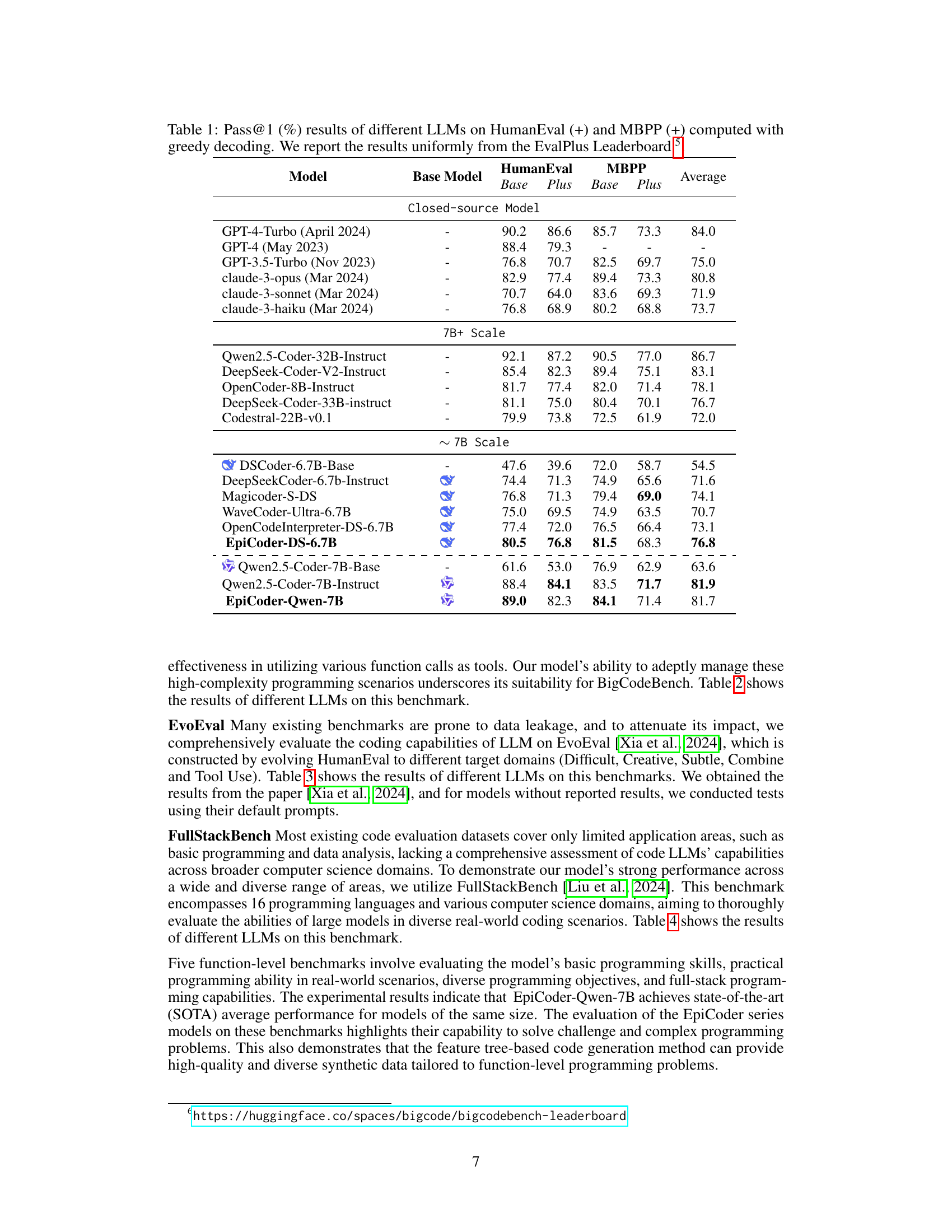
🔼 This table presents the pass@1 scores achieved by various Large Language Models (LLMs) on the BigCodeBench benchmark. BigCodeBench is a comprehensive benchmark designed to evaluate code generation capabilities across various programming tasks and domains. The evaluation was performed using greedy decoding and focused on both the ‘Full’ and ‘Hard’ subsets of the benchmark, which include ‘Complete’ and ‘Instruct’ tasks. The table highlights the performance differences between various LLMs, showcasing the relative strengths and weaknesses of each model. Scores not directly obtained from the BigCodeBench leaderboard (underlined in the table) were taken from the respective LLMs’ original papers, ensuring consistency in evaluation methodology.
read the caption
Table 2: Pass@1 (%) results of different LLMs on BigCodeBench computed with greedy decoding. We conducted the evaluation on the Full and Hard subsets of this benchmark, including the Complete and Instruct tasks. Except for the results underlined, which are sourced from their respective papers, all other results are obtained from the BigCodeBench-Leaderboard666https://huggingface.co/spaces/bigcode/bigcodebench-leaderboard.
| Model | Difficult | Creative | Subtle | Combine | Tool Use | Avg |
|---|---|---|---|---|---|---|
| Closed-source Model | ||||||
| GPT-4-Turbo | 50.0 | 61.0 | 82.0 | 45.0 | 69.0 | 61.4 |
| GPT-4 | 52.0 | 66.0 | 76.0 | 53.0 | 68.0 | 63.0 |
| Claude-3 | 50.0 | 53.0 | 81.0 | 42.0 | 69.0 | 59.0 |
| ChatGPT | 33.0 | 42.0 | 70.0 | 33.0 | 64.0 | 48.4 |
| Claude-3-haiku | 40.0 | 47.0 | 65.0 | 17.0 | 56.0 | 45.0 |
| 7B+ Scale | ||||||
| DeepSeekCoder-33b-Instruct | 47.0 | 47.0 | 67.0 | 31.0 | 66.0 | 51.6 |
| WizardCoder-33b-1.1 | 48.0 | 48.0 | 66.0 | 20.0 | 64.0 | 49.2 |
| CodeLlama-70b-Instruct | 31.0 | 41.0 | 65.0 | 18.0 | 65.0 | 44.0 |
| OpenCoder-8B-Instruct | 45.0 | 50.0 | 73.0 | 28.0 | 50.0 | 49.2 |
| ∼ 7B Scale | ||||||
| DeepSeek-Coder-6.7B-base | 21.0 | 24.0 | 47.0 | 5.0 | 55.0 | 30.4 |
| DeepSeekCoder-6.7b-Instruct | 40.0 | 37.0 | 61.0 | 18.0 | 51.0 | 41.4 |
| Magicoder-S-DS-6.7B | 40.0 | 34.0 | 67.0 | 21.0 | 61.0 | 44.6 |
| WaveCoder-Ultra-6.7B | 38.0 | 42.0 | 71.0 | 24.0 | 35.0 | 42.0 |
| OpenCodeInterpreter-DS-6.7B | 43.0 | 37.0 | 65.0 | 25.0 | 51.0 | 44.2 |
| EpiCoder-DS-6.7B | 40.0 | 45.0 | 70.0 | 30.0 | 65.0 | 50.0 |
| Qwen2.5-Coder-7B-Base | 35.0 | 20.0 | 55.0 | 27.0 | 41.0 | 35.6 |
| Qwen2.5-Coder-7B-Instruct | 48.0 | 49.0 | 77.0 | 37.0 | 65.0 | 55.2 |
| EpiCoder-Qwen-7B | 53.0 | 48.0 | 78.0 | 47.0 | 68.0 | 58.8 |
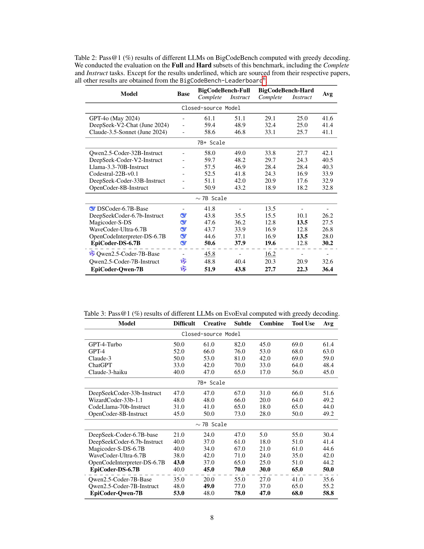
🔼 This table presents the pass@1 scores achieved by various Large Language Models (LLMs) on the EvoEval benchmark. EvoEval is a challenging code generation benchmark that tests a model’s ability to generalize across different coding tasks (difficult, creative, subtle, combined, and tool-use). The results illustrate the relative performance of each LLM in handling the complexity and diversity inherent in these tasks, showcasing strengths and weaknesses in code generation capabilities.
read the caption
Table 3: Pass@1 (%) results of different LLMs on EvoEval computed with greedy decoding.
| Model | BP | AP | SE | DP | MA | DW | ML | SC | DB | MM | OS | Others | Overall | |
|---|---|---|---|---|---|---|---|---|---|---|---|---|---|---|
| Close-Sourced API Model | ||||||||||||||
| OpenAI o1-preview | 55.56 | 78.61 | 64.29 | 76.80 | 79.14 | 18.75 | 51.28 | 61.76 | 40.00 | 47.37 | 100.00 | 74.47 | 66.47 | |
| OpenAI o1-mini | 72.22 | 75.62 | 50.00 | 76.00 | 80.58 | 28.75 | 56.41 | 56.62 | 40.00 | 57.89 | 100.00 | 72.34 | 66.23 | |
| Claude-35-Sonnet | 50.00 | 75.62 | 71.43 | 76.00 | 76.26 | 13.75 | 51.28 | 61.76 | 50.00 | 63.16 | 100.00 | 78.72 | 65.52 | |
| GPT 4o-0806 | 72.22 | 72.14 | 53.57 | 78.40 | 76.98 | 21.25 | 66.67 | 55.15 | 40.00 | 68.42 | 100.00 | 72.34 | 65.05 | |
| Doubao-Coder-Preview | 55.56 | 69.65 | 50.00 | 77.60 | 75.54 | 27.50 | 51.28 | 60.29 | 20.00 | 63.16 | 50.00 | 55.32 | 62.91 | |
| DeepSeek-v2.5 | 55.56 | 68.16 | 50.00 | 76.00 | 76.26 | 20.00 | 48.72 | 56.62 | 40.00 | 63.16 | 50.00 | 65.96 | 61.85 | |
| Qwen-Max | 50.00 | 70.15 | 39.29 | 77.60 | 72.66 | 13.75 | 56.41 | 57.35 | 30.00 | 47.37 | 50.00 | 63.83 | 60.78 | |
| GLM-4-Plus | 55.56 | 65.67 | 39.29 | 76.80 | 74.82 | 13.75 | 58.97 | 50.00 | 40.00 | 52.63 | 100.00 | 53.19 | 58.77 | |
| 20B+ Instruction Tuned Coder | ||||||||||||||
| DeepSeekCoder-v2-Instruct | 55.56 | 68.66 | 35.71 | 81.60 | 79.14 | 16.25 | 48.72 | 53.68 | 40.00 | 52.63 | 50.00 | 57.45 | 61.26 | |
| Qwen2.5-Coder-32B-Instruct | 50.00 | 70.15 | 50.00 | 77.60 | 66.19 | 17.50 | 61.54 | 43.38 | 30.00 | 47.37 | 100.00 | 61.70 | 58.41 | |
| DeepSeekCoder-33B-Instruct | 50.00 | 59.70 | 21.43 | 71.20 | 48.92 | 18.75 | 48.72 | 40.44 | 30.00 | 42.11 | 50.00 | 44.68 | 49.05 | |
| CodeLlama-34B-Instruct | 5.56 | 22.89 | 14.29 | 40.00 | 17.27 | 16.25 | 15.38 | 18.38 | 30.00 | 26.32 | 0.00 | 23.40 | 22.27 | |
| 13B+ Instruction Tuned Coder | ||||||||||||||
| Qwen2.5-Coder-14B-Instruct | 55.56 | 62.69 | 32.14 | 76.00 | 70.50 | 18.75 | 53.85 | 38.97 | 30.00 | 57.89 | 100.00 | 55.32 | 55.57 | |
| DeepSeekCoder-v2-Lite-Instruct | 50.00 | 64.68 | 32.14 | 64.00 | 56.12 | 26.25 | 43.59 | 33.82 | 60.00 | 21.05 | 50.00 | 53.19 | 50.47 | |
| StarCoder2-15B-Instruct-v0.1 | 61.11 | 44.28 | 32.14 | 63.20 | 36.69 | 31.25 | 53.85 | 28.68 | 60.00 | 36.84 | 50.00 | 53.19 | 43.01 | |
| CodeLlama-13B-Instruct | 11.11 | 22.39 | 25.00 | 24.00 | 20.86 | 30.00 | 20.51 | 13.97 | 40.00 | 10.53 | 50.00 | 23.40 | 21.56 | |
| 6B+ Instruction Tuned Coder | ||||||||||||||
| Qwen2.5-Coder-7B-Instruct | 33.33 | 58.21 | 39.29 | 66.40 | 48.92 | 18.75 | 38.46 | 32.35 | 40.00 | 47.37 | 50.00 | 59.57 | 47.51 | |
| Yi-Coder-9B-Chat | 61.11 | 50.25 | 32.14 | 66.40 | 46.76 | 26.25 | 43.59 | 36.76 | 50.00 | 36.84 | 50.00 | 48.94 | 46.56 | |
| DeepSeek-Coder-7B-Instruct-v1.5 | 50.00 | 51.74 | 25.00 | 64.80 | 37.41 | 25.00 | 30.77 | 34.56 | 20.00 | 52.63 | 50.00 | 48.94 | 43.60 | |
| OpenCoder-8B-Instruct | 44.44 | 53.73 | 28.57 | 57.60 | 35.97 | 26.25 | 28.21 | 28.68 | 0.00 | 47.37 | 0.00 | 44.68 | 41.11 | |
| DeepSeek-Coder-6.7B-Instruct | 61.11 | 49.75 | 28.57 | 65.60 | 38.13 | 18.75 | 38.46 | 22.79 | 30.00 | 31.58 | 50.00 | 42.55 | 40.88 | |
| CodeQwen1.5-7B-Chat | 38.89 | 45.77 | 50.00 | 58.40 | 31.65 | 15.00 | 33.33 | 22.79 | 20.00 | 31.58 | 0.00 | 42.55 | 37.20 | |
| CodeLlama-7B-Instruct | 27.78 | 23.88 | 25.00 | 28.00 | 20.86 | 23.75 | 10.26 | 11.76 | 50.00 | 10.53 | 0.00 | 21.28 | 21.33 | |
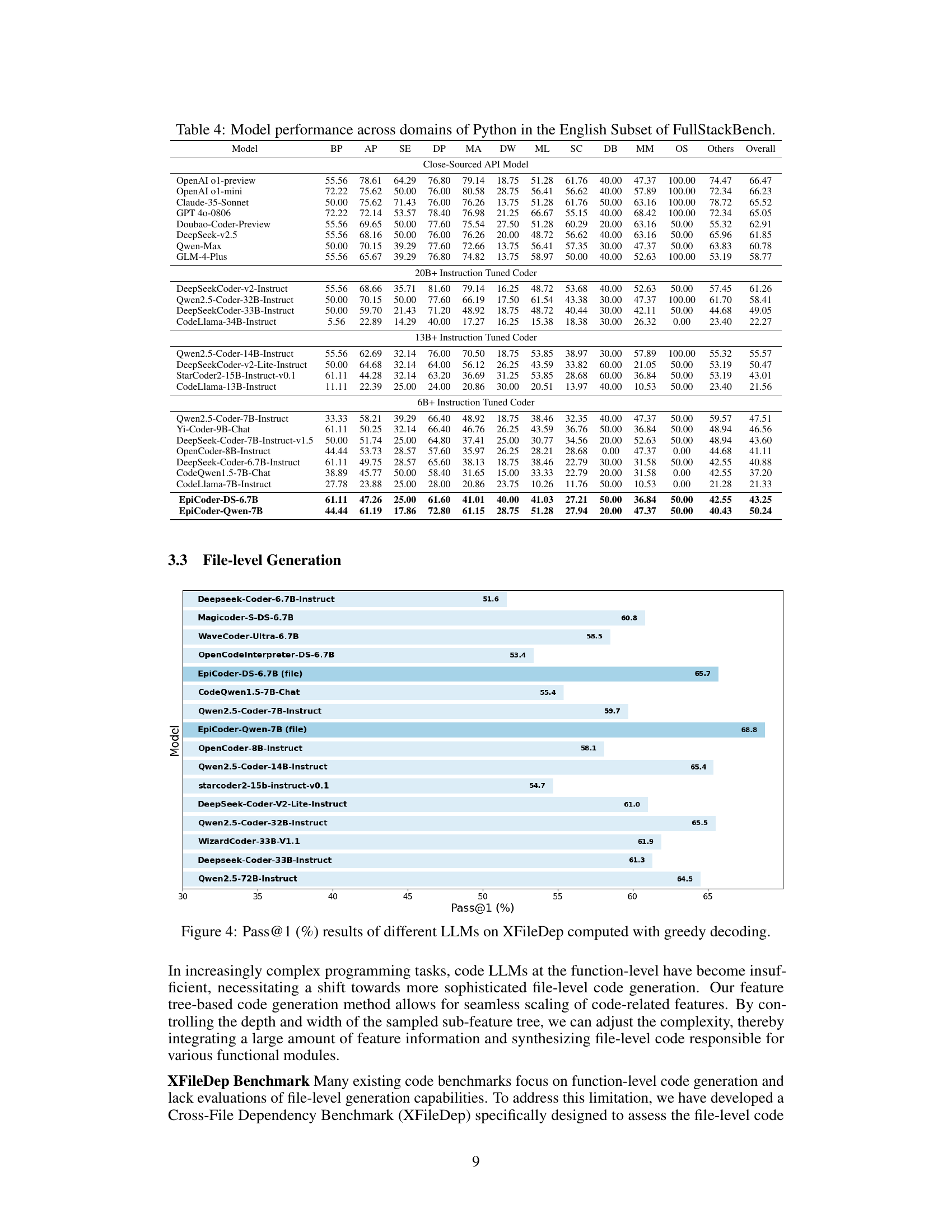
| EpiCoder-DS-6.7B | 61.11 | 47.26 | 25.00 | 61.60 | 41.01 | 40.00 | 41.03 | 27.21 | 50.00 | 36.84 | 50.00 | 42.55 | 43.25 | |
| EpiCoder-Qwen-7B | 44.44 | 61.19 | 17.86 | 72.80 | 61.15 | 28.75 | 51.28 | 27.94 | 20.00 | 47.37 | 50.00 | 40.43 | 50.24 |
🔼 This table presents a comprehensive evaluation of various large language models (LLMs) on the FullStackBench benchmark, specifically focusing on their performance in different domains of Python programming within the English subset of the benchmark. It assesses the models’ capabilities across a diverse range of tasks and programming styles, providing a detailed breakdown of their performance in various sub-domains. The results offer insights into the strengths and weaknesses of each model, highlighting their proficiency in handling diverse programming challenges.
read the caption
Table 4: Model performance across domains of Python in the English Subset of FullStackBench.
| Dataset | Unique Operators | Unique Operands | Total Operators | Total Operands |
|---|---|---|---|---|
| Code Alpaca [Chaudhary (2023)] | 4.83 | 8.22 | 10.66 | 15.89 |
| Evol CodeAlpaca [Luo et al. (2023)] | 7.94 | 18.97 | 29.91 | 46.70 |
| CodeFeedBack [Zheng et al. (2024b)] | 8.11 | 20.42 | 30.98 | 50.05 |
| OSS Instruct [Wei et al. (2024b)] | 7.44 | 20.99 | 28.05 | 47.55 |
| Ours (func-level) | 10.66 | 44.32 | 56.98 | 100.36 |
| Ours (file-level) | 11.64 | 72.87 | 100.24 | 179.98 |
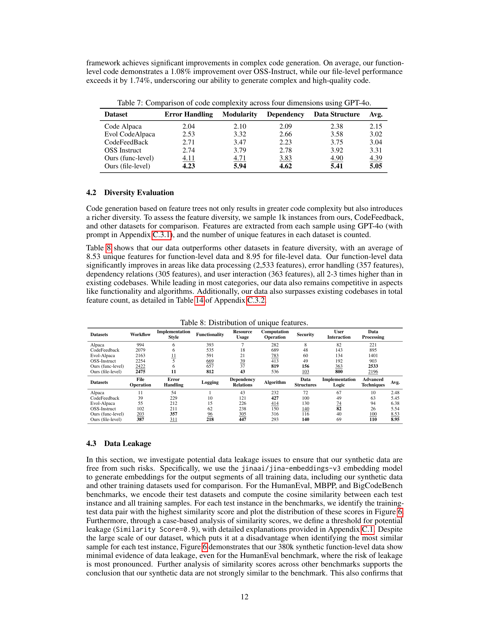
🔼 This table presents a comparison of Halstead complexity metrics between the synthetic code data generated by the proposed method and several existing code datasets. The Halstead complexity metrics used are: unique operators (n1), unique operands (n2), total operators (N1), and total operands (N2). The table highlights the differences in code complexity between the newly generated dataset and other datasets, showing that the proposed method generates code with significantly higher Halstead complexity, indicating a greater level of complexity and potentially a higher level of difficulty in the generated code.
read the caption
Table 5: Comparison of Halstead complexity between ours and existing codebase.
| Dataset | Mean | Median | Std |
|---|---|---|---|
| Code Alpaca | 0.18 | 0.00 | 0.52 |
| Evol CodeAlpaca | 0.82 | 0.00 | 1.63 |
| CodeFeedBack | 0.97 | 0.00 | 2.09 |
| OSS Instruct | 1.50 | 1.00 | 2.19 |
| Ours (func-level) | 4.95 | 4.00 | 3.77 |
| Ours (file-level) | 5.41 | 4.00 | 3.85 |
🔼 This table presents a comparison of code complexity metrics, specifically Strictness and Cyclomatic complexity, across several datasets. Strictness Complexity measures how strictly the code adheres to a single execution path, while Cyclomatic Complexity assesses the control flow complexity, indicating the number of linearly independent paths through the code. By comparing these metrics across different datasets (Code Alpaca, Evol CodeAlpaca, CodeFeedBack, OSS Instruct, and the authors’ own function-level and file-level datasets), the table allows for an evaluation of the relative complexity of the code generated by each method. The use of median and standard deviation provide a robust statistical analysis of the complexity scores.
read the caption
Table 6: Comparison of Strictness complexity (left) and Cyclomatic complexity (right).
| Dataset | Mean | Median | Std |
|---|---|---|---|
| Code Alpaca | 2.10 | 1.00 | 1.66 |
| Evol CodeAlpaca | 3.76 | 3.00 | 3.48 |
| CodeFeedBack | 3.96 | 3.00 | 3.33 |
| OSS Instruct | 3.45 | 3.00 | 2.98 |
| Ours (func-level) | 5.14 | 5.00 | 3.01 |
| Ours (file-level) | 14.93 | 14.00 | 6.73 |
🔼 This table presents a quantitative comparison of code complexity across four key dimensions: Error Handling, Modularity, Dependency, and Data Structure. The complexity of code samples from different datasets is evaluated using GPT-40, a large language model, which assigns a score to each sample based on predefined standards for each dimension. Higher scores indicate greater complexity.
read the caption
Table 7: Comparison of code complexity across four dimensions using GPT-4o.
| Dataset | Error Handling | Modularity | Dependency | Data Structure | Avg. |
|---|---|---|---|---|---|
| Code Alpaca | 2.04 | 2.10 | 2.09 | 2.38 | 2.15 |
| Evol CodeAlpaca | 2.53 | 3.32 | 2.66 | 3.58 | 3.02 |
| CodeFeedBack | 2.71 | 3.47 | 2.23 | 3.75 | 3.04 |
| OSS Instruct | 2.74 | 3.79 | 2.78 | 3.92 | 3.31 |
| Ours (func-level) | 4.11 | 4.71 | 3.83 | 4.90 | 4.39 |
| Ours (file-level) | 4.23 | 5.94 | 4.62 | 5.41 | 5.05 |
🔼 This table presents a quantitative analysis of the diversity of features extracted from different code datasets using a large language model (LLM). It breaks down the number of unique features found across various categories, such as workflow, implementation style, functionality, resource usage, and data processing, offering insights into the richness and variety of the code samples represented in each dataset. This analysis is crucial for evaluating the quality and representativeness of the training data used to train large language models (LLMs) for code generation.
read the caption
Table 8: Distribution of unique features.
| Datasets | Workflow | Implementation | Style | Functionality | Resource | Usage | Computation | Operation | Security | User | Interaction | Data | Processing | Avg. |
|---|---|---|---|---|---|---|---|---|---|---|---|---|---|---|
| Alpaca | 994 | 6 | 393 | 7 | 282 | 8 | 82 | 221 | 11 | 54 | 1 | 43 | 2.48 | |
| CodeFeedback | 2079 | 6 | 535 | 18 | 689 | 48 | 143 | 895 | 39 | 229 | 10 | 121 | 5.45 | |
| Evol-Alpaca | 2163 | 11 | 591 | 21 | 783 | 60 | 134 | 1401 | 55 | 212 | 15 | 226 | 6.38 | |
| OSS-Instruct | 2254 | 5 | 669 | 39 | 413 | 49 | 192 | 903 | 102 | 211 | 62 | 238 | 5.54 | |
| Ours (func-level) | 2422 | 6 | 657 | 37 | 819 | 156 | 363 | 2533 | 203 | 357 | 96 | 305 | 8.53 | |
| Ours (file-level) | 2475 | 11 | 812 | 43 | 536 | 103 | 800 | 2196 | 387 | 311 | 218 | 447 | 8.95 |
🔼 This table presents a quantitative comparison of the number of test functions and test cases in the XFileDep benchmark dataset before and after data augmentation. It shows the total counts, averages per sample, and maximum counts found within individual files. The augmentation process significantly increased both the number of test functions and test cases, improving the overall coverage and robustness of the benchmark.
read the caption
Table 9: Comparison of Test Functions and Test Cases before and after augmentation for 930 data samples.
| Implementation | Style |
|---|
🔼 This table shows the indices of specific data samples used in a case study on data leakage analysis. The case study examines the similarity between samples from the HumanEval benchmark dataset and the evol-codealpaca-v1 dataset. The table presents four similarity scores (99%, 95%, 90%, and 85%) and lists the corresponding indices from both datasets for each score, illustrating the degree of similarity between the benchmark and training data at various levels.
read the caption
Table 10: The index of the data samples presented in the case study.
| Resource | Usage |
|---|
🔼 This table presents a detailed comparison of Halstead complexity metrics across different code datasets. Halstead metrics quantify software complexity based on counts of unique and total operators and operands. The table shows the values for program length, vocabulary, volume, and difficulty for each dataset. This allows for a quantitative comparison of the complexity of different codebases, highlighting the relative complexity of the datasets.
read the caption
Table 11: Derived Halstead metrics. These metrics are derived from unique operators (n1subscript𝑛1n_{1}italic_n start_POSTSUBSCRIPT 1 end_POSTSUBSCRIPT), unique operands (n2subscript𝑛2n_{2}italic_n start_POSTSUBSCRIPT 2 end_POSTSUBSCRIPT), total operators (N1subscript𝑁1N_{1}italic_N start_POSTSUBSCRIPT 1 end_POSTSUBSCRIPT), and total operands (N2subscript𝑁2N_{2}italic_N start_POSTSUBSCRIPT 2 end_POSTSUBSCRIPT).
| Computation | Operation |
|---|
🔼 This table presents a quantitative comparison of the frequencies of various control flow and logical operations across different code datasets. It shows the counts of ‘if’, ‘while’, ‘for’, ‘and’, ‘or’, ’except’, ‘return’, ‘break’, ‘continue’, and ‘bool_op’ statements within the code. The datasets compared include Code Alpaca, Evol Code Alpaca, CodeFeedBack, OSS Instruct, and the authors’ own function-level and file-level datasets. The table helps to illustrate the differences in code complexity and style across different datasets, highlighting aspects like the use of loops, exception handling, and boolean logic.
read the caption
Table 12: Comparison of different control flow and logical operation frequencies.
| User | Interaction |
|---|
🔼 This table presents a detailed breakdown of code strictness complexity metrics across different datasets. It goes beyond a simple count and examines various aspects related to code quality and rigor, such as exception handling, documentation (docstrings), input validation, type hinting, and assertion usage. This granular analysis allows for a more nuanced comparison of code quality across datasets, offering insights into the adherence to best practices and coding standards. The values likely represent frequencies or percentages of these features in the code samples from each dataset.
read the caption
Table 13: Detailed metrics of code strictness complexity
| Data | Processing |
|---|
🔼 This table presents a detailed breakdown of the feature diversity observed in 1,000 samples from various code datasets. It compares the distribution of features across different categories, such as workflow, implementation, resource usage, and data processing, offering a quantitative assessment of the richness and variety of code characteristics represented within each dataset. The datasets included are Alpaca, CodeFeedback, Evol-Alpaca, OSS-Instruct, and two versions of data generated by the authors’ method (function-level and file-level). This comparison highlights the relative complexity and diversity of code features within each data source, providing valuable insight for assessing the suitability of different datasets for training code generation models.
read the caption
Table 14: Distribution of total features across 1k samples.
Full paper#
