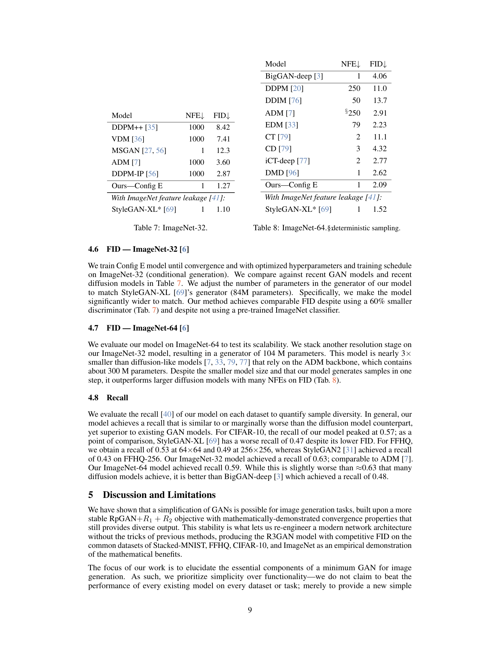
↗ arXiv ↗ Hugging Face ↗ Papers with Code
TL;DR#
Generative Adversarial Networks (GANs) have gained popularity for generating high-quality images, but they’ve been known for their training instability and reliance on numerous empirical tricks. These tricks often address issues like mode collapse (where the generator produces limited variety of images) and mode dropping (where the generator fails to capture all the modes of data distribution). These issues have hindered GAN’s widespread adoption and scalability.
This research introduces R3GAN, a new GAN baseline that tackles these long-standing problems head-on. By deriving a well-behaved regularized loss function and replacing outdated GAN backbones with modern architectures, R3GAN simplifies the GAN training process, discards previous ad-hoc tricks, and achieves state-of-the-art results on various benchmark datasets, outperforming even StyleGAN2 and some diffusion models in terms of FID score and mode coverage. This significantly simplifies GAN training, improves its stability and performance, and provides a new foundation for future research.
Key Takeaways#
Why does it matter?#
This paper is crucial because it challenges the common belief that GANs are notoriously difficult to train. By introducing a novel, mathematically-sound loss function and modern architectures, it provides a simpler, more stable, and higher-performing GAN baseline. This simplifies GAN research, making it more accessible and paving the way for more advanced models. It also challenges the dominance of diffusion models, suggesting GANs can still compete, even with simpler designs. The work opens up new directions for improving GAN training stability and scalability, as well as furthering research in generative modeling in general.
Visual Insights#

🔼 The figure shows the Generator’s loss curves during training for various GAN loss functions. The x-axis represents the training time, and the y-axis represents the Generator’s loss. Different lines represent different loss functions, including the combination of RpGAN loss with different gradient penalties (R1 and/or R2). The plot highlights the instability of GAN training when using only the R1 gradient penalty, leading to divergence. However, the combination of R1 and R2 penalties results in stable training and convergence, which is consistent with the theoretical analysis presented in the paper.
read the caption
Figure 1: Generator G𝐺Gitalic_G loss for different objectives over training. Regardless of which objective is used, training diverges with only R1subscript𝑅1R_{1}italic_R start_POSTSUBSCRIPT 1 end_POSTSUBSCRIPT and succeeded with both R1subscript𝑅1R_{1}italic_R start_POSTSUBSCRIPT 1 end_POSTSUBSCRIPT and R2subscript𝑅2R_{2}italic_R start_POSTSUBSCRIPT 2 end_POSTSUBSCRIPT. Convergence failure with only R1subscript𝑅1R_{1}italic_R start_POSTSUBSCRIPT 1 end_POSTSUBSCRIPT was noted by Lee et al. [42].
| Loss | # modes ↑ | DKL ↓ |
|---|---|---|
| RpGAN +R1+R2 | 1000 | 0.0781 |
| GAN +R1+R2 | 693 | 0.9270 |
| RpGAN +R1 | Fail | Fail |
| GAN +R1 | Fail | Fail |
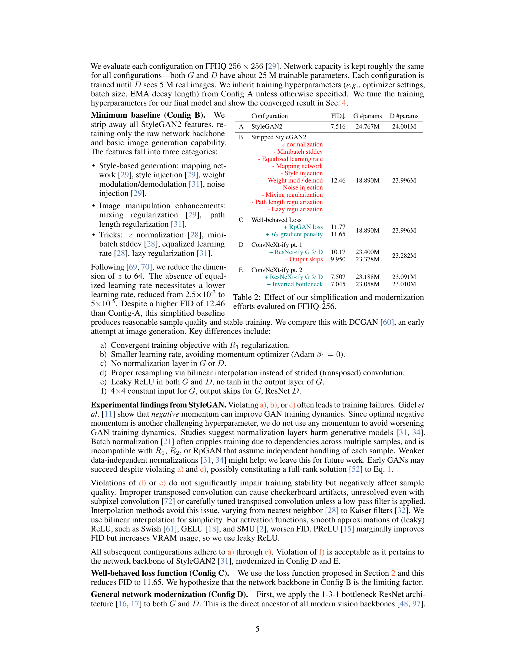
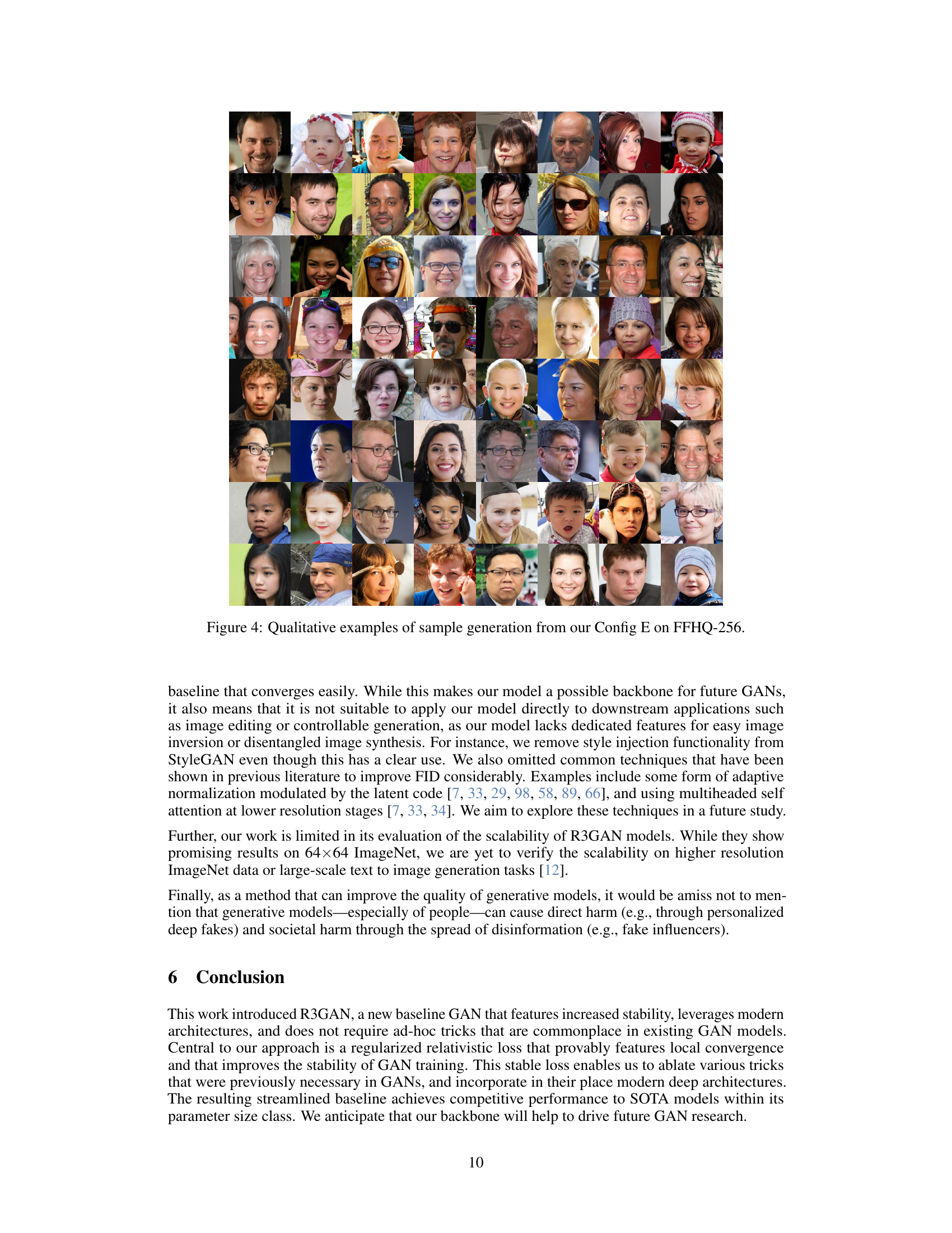
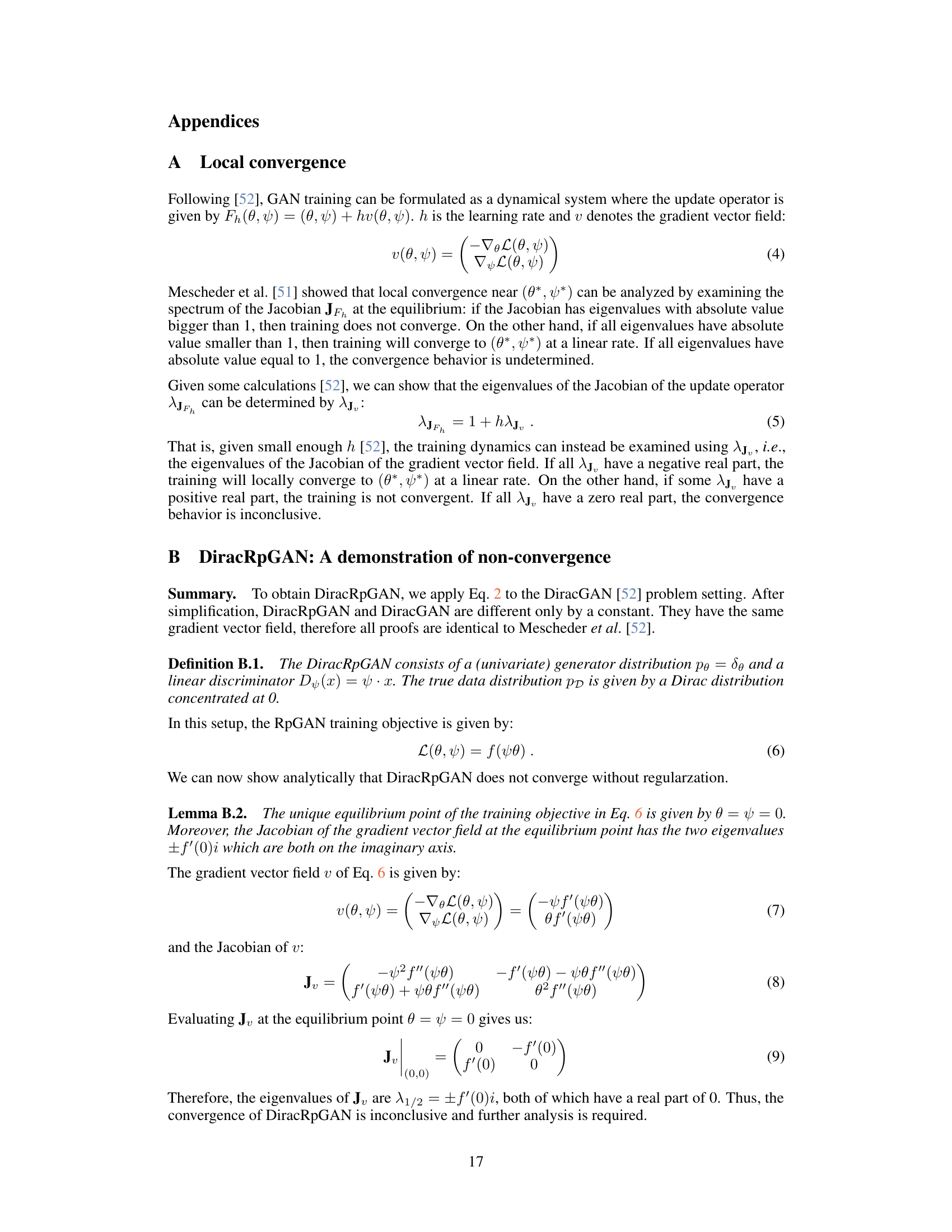
🔼 This table presents the results of a series of experiments conducted on the FFHQ-256 dataset to evaluate the impact of simplifying and modernizing the StyleGAN2 architecture. It compares several configurations, starting with the original StyleGAN2 and progressively removing features (tricks) and updating the backbone architecture with modern components. The configurations are denoted as Config A through Config E, with Config A representing the original StyleGAN2, and Config E representing the final, simplified and modernized model. The table shows the Fréchet Inception Distance (FID), which measures the quality of generated images, and the number of trainable parameters for both the generator (G) and discriminator (D) in each configuration. The results illustrate how the removal of unnecessary features and the incorporation of modern architectural designs can improve the performance of GANs while reducing the complexity of the model.
read the caption
Table 1: Effect of our simplification and modernization efforts evaluted on FFHQ-256.
In-depth insights#
GAN Training Issues#
Generative Adversarial Networks (GANs) have shown remarkable potential in generating high-quality images, but their training process is notoriously unstable and challenging. Mode collapse, where the generator produces limited variations of images, is a significant issue. Non-convergence, where the generator and discriminator fail to reach an equilibrium, is another major obstacle. The original GAN objective function suffers from a minimax game formulation, prone to vanishing or exploding gradients. Furthermore, achieving a balance between diversity and stability is crucial but difficult. Existing GAN architectures frequently incorporate numerous empirical tricks and heuristics to mitigate these problems, lacking a rigorous theoretical foundation. These issues contribute to the perceived difficulty of GAN training, hindering progress and adoption.
R3GAN: A New Baseline#
The proposed R3GAN aims to establish a modern baseline for Generative Adversarial Networks (GANs), challenging the common perception of GANs as notoriously difficult to train. R3GAN achieves this by focusing on a well-behaved, mathematically-grounded loss function, derived from a regularized relativistic GAN loss. This robust loss eliminates the need for many ad-hoc training tricks that plague other GAN architectures. Furthermore, R3GAN leverages modern convolutional neural network backbones, updating the outdated architectures frequently found in SOTA GANs. The result is a simple, effective GAN architecture that outperforms StyleGAN2 and other competitive GANs and diffusion models across various datasets. This suggests that the complexity associated with GAN training might be significantly reduced by focusing on fundamental theoretical improvements rather than relying on numerous empirical fixes.
Modern GAN Architectures#
Modern GAN architectures represent a significant evolution from their predecessors, focusing on improved training stability and enhanced sample quality. Key advancements include the adoption of residual networks and other convolutional neural network designs to facilitate training deeper and wider networks. This allows for greater expressivity in generated images while mitigating issues like mode collapse. StyleGAN’s introduction of a style-based generator architecture is another pivotal contribution, enabling more intricate control over the generation process. Further improvements have incorporated techniques like attention mechanisms (as seen in transformer-based GANs) and improved regularization methods, further addressing the historical challenges of GAN training such as non-convergence and instability. Progressive growing of GANs also helps to improve stability by gradually increasing the resolution of generated images. These methods collectively address limitations of older GAN architectures, leading to higher fidelity image generation and superior sample diversity. The ongoing research into modern GANs continuously pushes the boundaries of generative modeling, and future advancements will likely further refine these architectural innovations.
Empirical Evaluation#
An empirical evaluation section in a research paper would typically present a comprehensive assessment of the proposed method’s performance. It should include details on the datasets used, metrics employed (e.g., FID, Inception Score, precision, recall), and a comparison against relevant baselines or state-of-the-art approaches. Rigorous statistical analysis, such as error bars or confidence intervals, is essential to demonstrate the significance of any observed improvements or differences. The choice of metrics should be justified based on their relevance to the problem being addressed, and the evaluation should account for any potential limitations or biases in the datasets or evaluation procedures. Ablation studies systematically removing components of the proposed model to isolate the contributions of each part would showcase the effectiveness of design decisions. Additionally, qualitative results, such as generated images or other outputs, can provide valuable insights and support quantitative findings, offering a more holistic view of the model’s capabilities. The discussion should clearly state whether the empirical findings validate the hypothesis or theoretical claims of the paper, and explore any unexpected or noteworthy results.
Future Research#
Future research directions stemming from this work could explore several promising avenues. Improving the scalability of R3GAN to higher-resolution datasets and larger-scale tasks like text-to-image generation is crucial. Investigating the use of attention mechanisms within the R3GAN architecture warrants attention, potentially enhancing the model’s ability to capture intricate details and improve sample quality. Further analysis into the theoretical properties of the regularized loss and its impact on training dynamics would deepen the understanding of R3GAN’s success. Finally, exploring alternative activation functions beyond ReLU, and investigating adaptive normalization techniques, could refine the model, potentially improving FID scores and sample diversity. A key focus should be to understand how architectural choices affect the balance between training stability and model expressiveness.
More visual insights#
More on figures
🔼 This figure shows the results of an experiment on the StackedMNIST dataset, which consists of 1000 uniformly distributed modes. Different loss functions were used to train a GAN, and the figure displays the maximum mode coverage achieved by each loss function. The maximum possible mode coverage is 1000, meaning that a perfect GAN would capture all 1000 modes. The ‘Fail’ entries indicate cases where the training process diverged early on, preventing the GAN from reaching a satisfactory solution.
read the caption
Figure 2: StackedMNIST [46] result for each loss function. The maximum possible mode coverage is 1000. “Fail” indicates that training diverged early on.
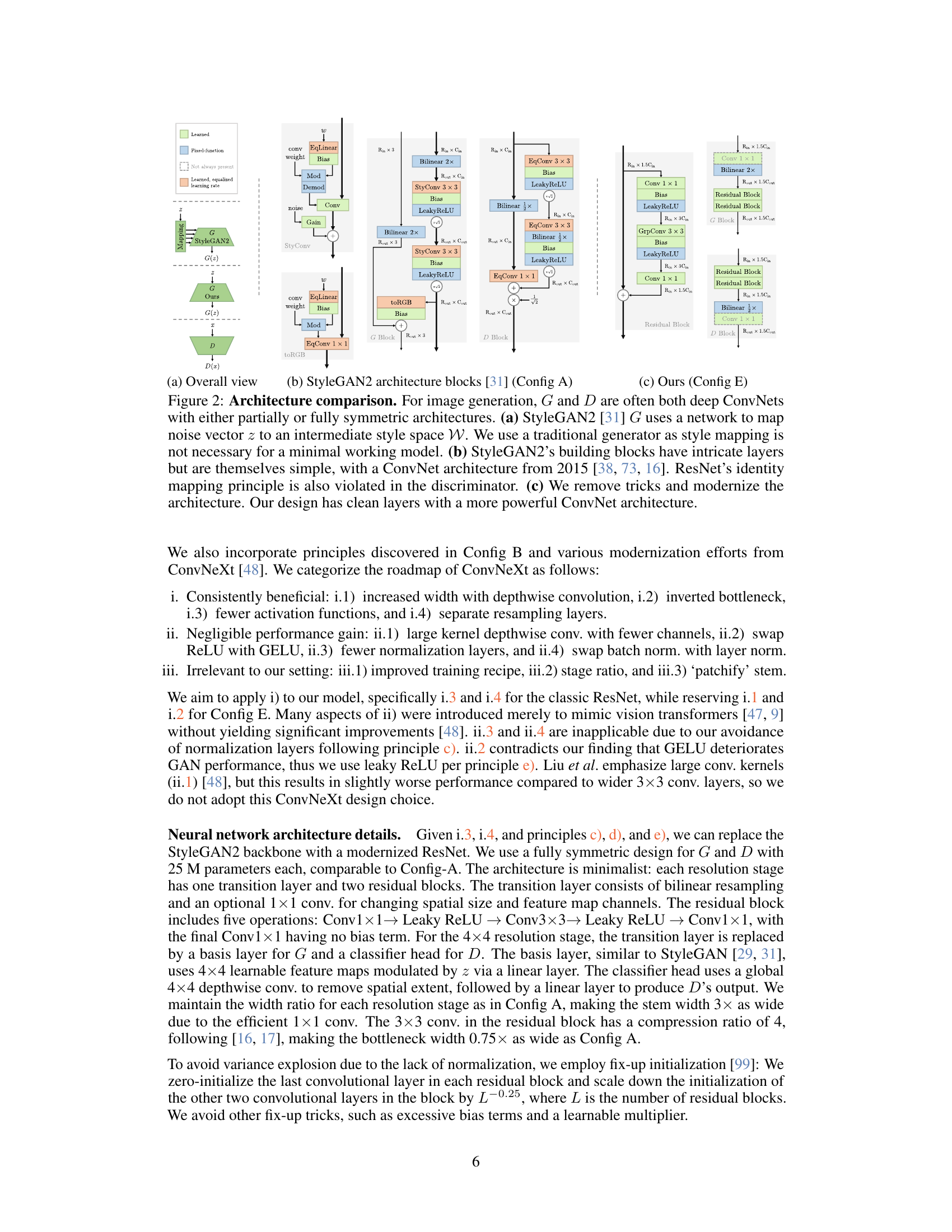
🔼 Figure 3 provides a detailed comparison of the architectures used in StyleGAN2 and the proposed R3GAN model for image generation. StyleGAN2’s architecture (part (b)) is presented as complex due to its reliance on intricate layers and features. Part (a) provides a simple comparison between the generator and discriminator of both models, and highlights some of the differences such as the style-mapping network in StyleGAN2 which is absent from R3GAN. The proposed R3GAN architecture (part (c)) is described as minimalist and modern, emphasizing its use of cleaner, more powerful ConvNet layers compared to StyleGAN2.
read the caption
Figure 3: Architecture comparison. For image generation, G𝐺Gitalic_G and D𝐷Ditalic_D are often both deep ConvNets with either partially or fully symmetric architectures. (a) StyleGAN2 [31] G𝐺Gitalic_G uses a network to map noise vector z𝑧zitalic_z to an intermediate style space 𝒲𝒲\mathcal{W}caligraphic_W. We use a traditional generator as style mapping is not necessary for a minimal working model. (b) StyleGAN2’s building blocks have intricate layers but are themselves simple, with a ConvNet architecture from 2015 [38, 73, 16]. ResNet’s identity mapping principle is also violated in the discriminator. (c) We remove tricks and modernize the architecture. Our design has clean layers with a more powerful ConvNet architecture.

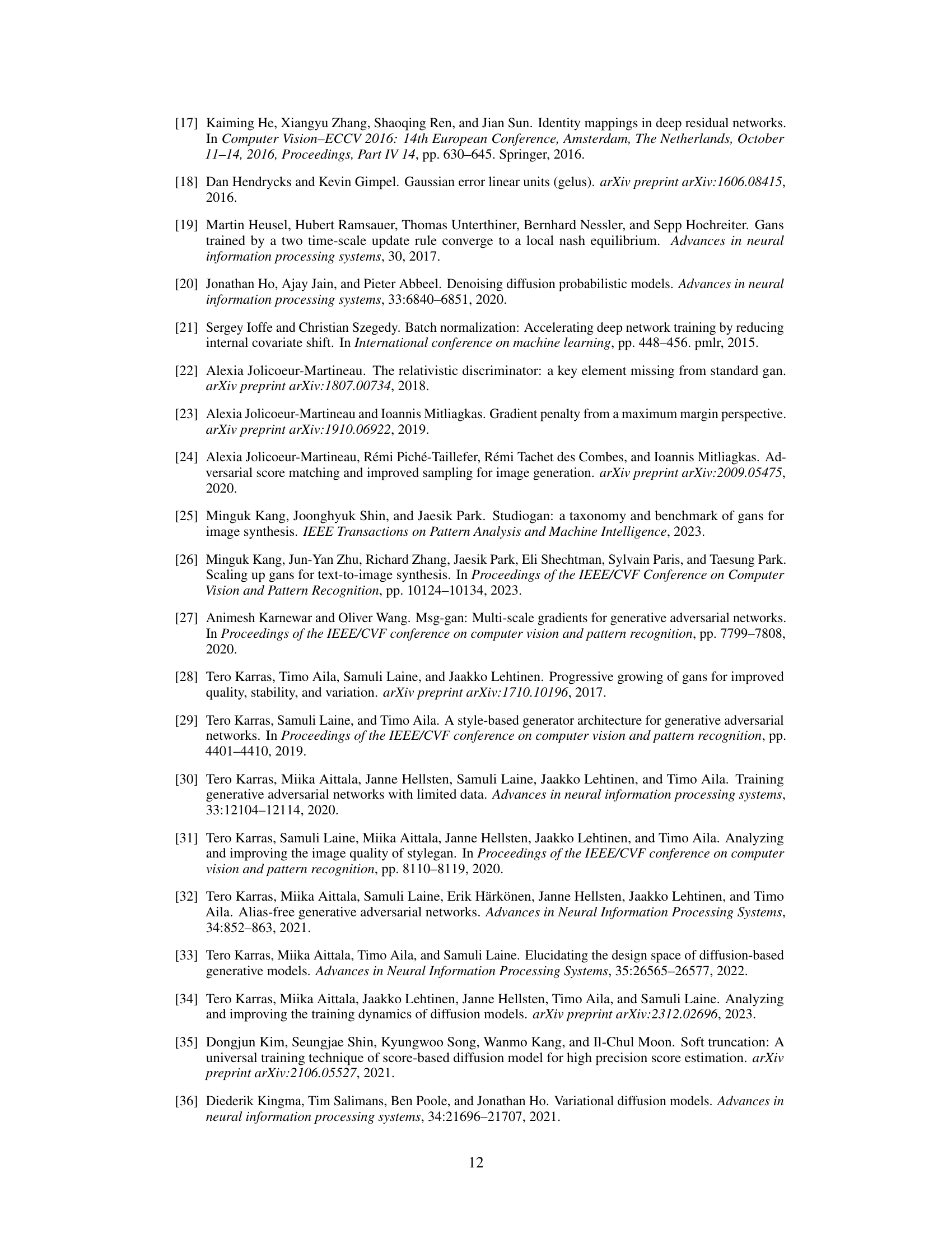
🔼 Figure 4 presents qualitative samples generated by the R3GAN model (Config E) on the FFHQ-256 dataset. It showcases the visual quality of images produced by the model, highlighting the realism and diversity achieved through the proposed method. This figure visually demonstrates the capabilities of the simplified and modernized GAN architecture introduced in the paper.
read the caption
Figure 4: FFHQ-256. * denotes models that leak ImageNet features.

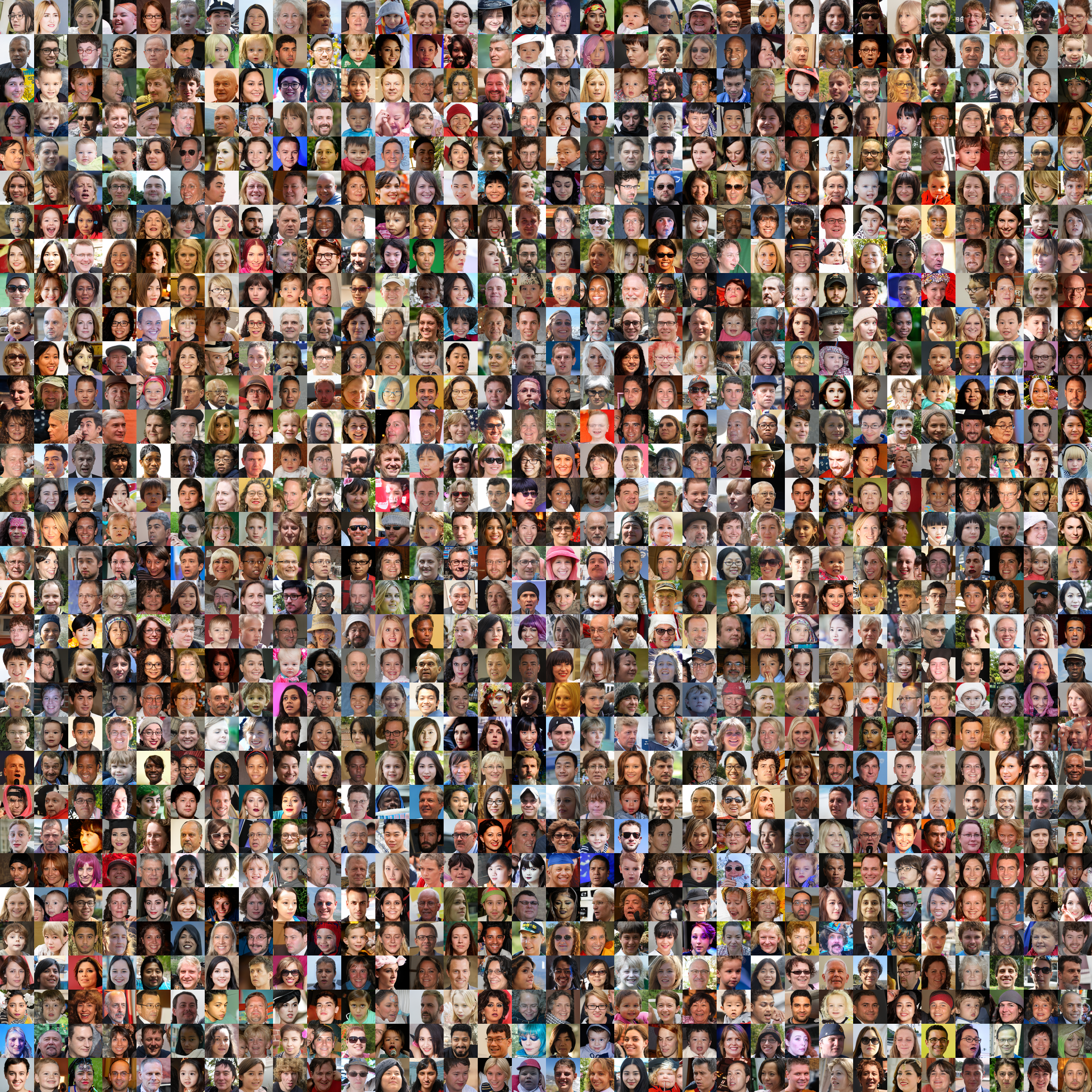
🔼 Figure 5 displays several images generated by the R3GAN model on the FFHQ-64 dataset. FFHQ-64 refers to the high-resolution Flickr Faces-HQ dataset, downsampled to 64x64 pixels. This figure showcases the model’s ability to generate realistic-looking faces at this lower resolution, demonstrating its capacity for generating high-quality images across different resolutions. The images represent a range of facial features and expressions, highlighting the diversity of the model’s output. The figure visually complements the quantitative results presented in the paper, providing evidence of the model’s performance in terms of image generation quality and variety.
read the caption
Figure 5: FFHQ-64.

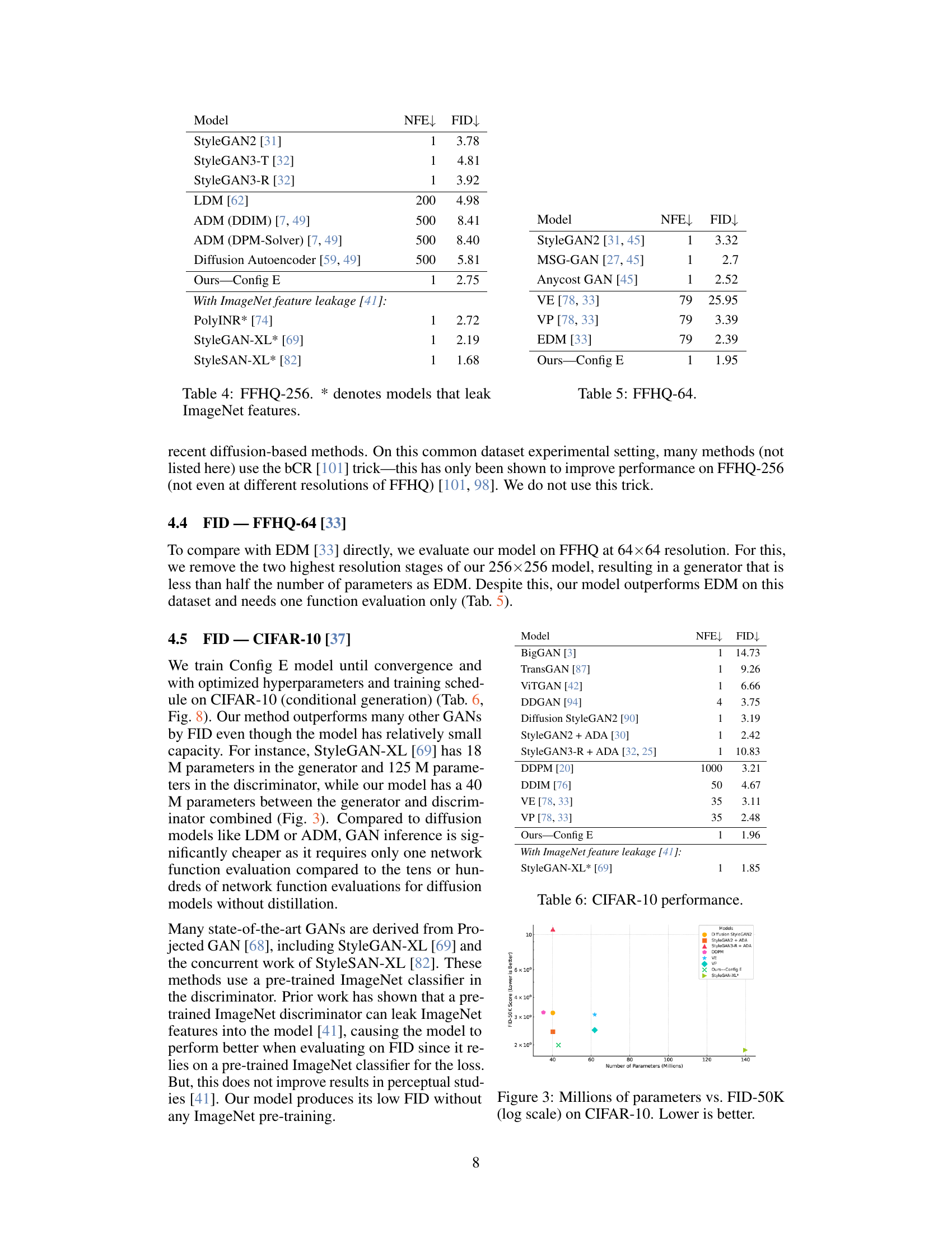
🔼 This figure shows the relationship between the number of parameters in a generative model and its performance on the CIFAR-10 dataset, measured by the Fréchet Inception Distance (FID) score. The x-axis represents the number of parameters (in millions) on a logarithmic scale, while the y-axis shows the FID score. A lower FID indicates better performance, meaning that the generated images are more realistic and similar to real images from the dataset. The plot allows for a comparison of different models’ efficiency in terms of parameter usage and image quality.
read the caption
Figure 6: Millions of parameters vs. FID-50K (log scale) on CIFAR-10. Lower is better.
More on tables
| Configuration | FID↓ | G #params | D #params |
|---|---|---|---|
| StyleGAN2 | 7.516 | 24.767M | 24.001M |
| Stripped StyleGAN2 | |||
| - z normalization - Minibatch stddev - Equalized learning rate - Mapping network - Style injection - Weight mod / demod - Noise injection - Mixing regularization - Path length regularization - Lazy regularization | 12.46 | 18.890M | 23.996M |
| Well-behaved Loss | 12.46 | 18.890M | 23.996M |
| + RpGAN loss | 11.77 | 18.890M | 23.996M |
| + R2 gradient penalty | 11.65 | 18.890M | 23.996M |
| ConvNeXt-ify pt. 1 | |||
| + ResNet-ify G & D | 10.17 | 23.400M | 23.282M |
| - Output skips | 9.950 | 23.378M | 23.282M |
| ConvNeXt-ify pt. 2 | |||
| + ResNeXt-ify G & D | 7.507 | 23.188M | 23.091M |
| + Inverted bottleneck | 7.045 | 23.058M | 23.010M |
🔼 This table presents the results of an experiment conducted on the StackedMNIST dataset, which consists of 1000 uniformly distributed modes. The experiment evaluated different loss functions, specifically different combinations of RpGAN (relativistic pairing GAN), R1, and R2 regularization, to assess their impact on the training dynamics of a GAN and its ability to capture all modes of the data. The table shows the number of modes covered by the generator (out of a possible 1000) and the reverse Kullback-Leibler (KL) divergence between the generated and true distributions, indicating how well the generator captures the true data distribution. The results illustrate the importance of regularization for GAN stability and mode coverage, highlighting the effectiveness of combining RpGAN with both R1 and R2 for achieving better results.
read the caption
Table 2: StackedMNIST 1000-mode coverage.
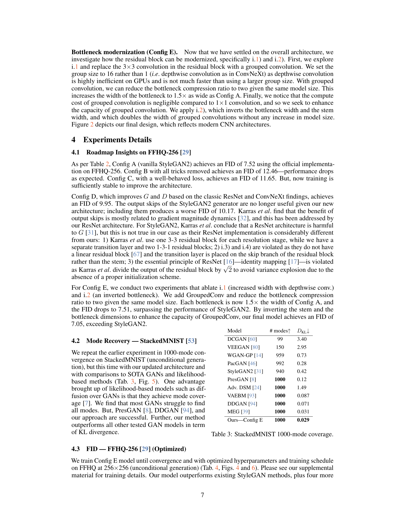
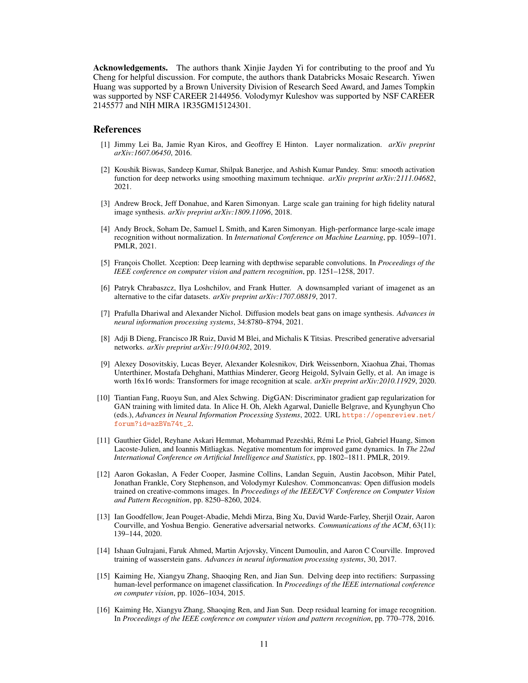
🔼 This table presents a comparison of the Fréchet Inception Distance (FID) scores achieved by various generative models on the CIFAR-10 dataset. It shows how the FID, a metric reflecting image quality and diversity, varies across different GAN (Generative Adversarial Network) and diffusion models, including both models using and not using ImageNet pre-training (indicated by *). The table helps illustrate the performance of the proposed model (Ours-Config E) compared to existing state-of-the-art models.
read the caption
Table 3: CIFAR-10 performance.
🔼 This table details the hyperparameters used in the experiments across different datasets (Stacked MNIST, CIFAR-10, FFHQ, and ImageNet). It includes settings such as resolution, whether class conditioning was used, the number of GPUs employed, the total training time (measured in millions of images), the burn-in period, minibatch size, learning rate schedule, R1 and R2 regularization parameters (and their decay), Adam’s beta2 parameter, EMA half-life (in millions of images), the number of residual blocks and groups per resolution, model parameter counts for both the generator (G) and discriminator (D), data augmentation (horizontal flips), and the schedule for augmentation probability. The formula for calculating the EMA decay factor (beta) is provided and an example calculation is given for the CIFAR-10 experiment.
read the caption
Table 4: Hyperparameters for each experiment. The decay factor β𝛽\betaitalic_β of EMA can be obtained using the formula β=0.5Minibatch sizeEMA half-life𝛽superscript0.5Minibatch sizeEMA half-life\beta=0.5^{\frac{\text{Minibatch size}}{\text{EMA half-life}}}italic_β = 0.5 start_POSTSUPERSCRIPT divide start_ARG Minibatch size end_ARG start_ARG EMA half-life end_ARG end_POSTSUPERSCRIPT, e.g. for CIFAR-10, EMA β=0.55125×10⁶≈0.9999𝛽superscript0.55125superscript1060.9999\beta=0.5^{\frac{512}{5\times 10^{6}}}\approx 0.9999italic_β = 0.5 start_POSTSUPERSCRIPT divide start_ARG 512 end_ARG start_ARG 5 × 10 start_POSTSUPERSCRIPT 6 end_POSTSUPERSCRIPT end_ARG end_POSTSUPERSCRIPT ≈ 0.9999.
Full paper#
