↗ arXiv ↗ Hugging Face ↗ Papers with Code
TL;DR#
Current video understanding models often lack the effectiveness of their text-based counterparts. This paper tackles this challenge by introducing a new approach: autoregressive pre-training directly from videos. The researchers used a large and diverse dataset, exceeding 1 trillion visual tokens, to train their models. The main challenge they faced was the lack of inherent sequential structure in video data compared to text, which they overcame using a raster scan approach. The study highlights a significant limitation of relying solely on internet videos because of their variability in quality and diversity.
The paper proposes a family of autoregressive video models called “Toto.” They tested the models’ effectiveness on various downstream tasks like image recognition, video classification, and object tracking, demonstrating competitive results despite minimal inductive bias. They discovered that their model scales similarly to language models, although at a different rate. The research also analyzed the impact of design choices like tokenizers and pooling methods, and found attention pooling to significantly outperform average pooling. These findings offer crucial insights into building efficient and effective video AI systems.
Key Takeaways#
Why does it matter?#
This paper is crucial for researchers in computer vision and video processing. It introduces a novel autoregressive pre-training approach for video models, showing scalable performance across various tasks. This opens up new avenues for large-scale video understanding and advances the field towards more efficient and effective video AI.
Visual Insights#

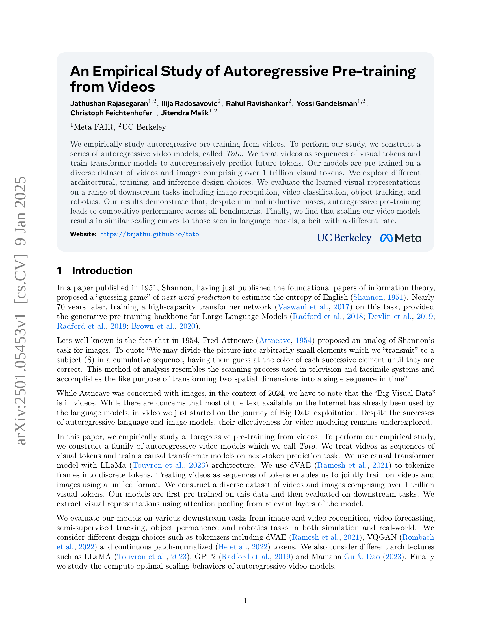
🔼 This figure illustrates the overall framework of the research, detailing the process from data acquisition to downstream task evaluation. The process begins with collecting images and video frames from various datasets. Each image and frame is then independently tokenized into a sequence of discrete visual tokens. A transformer model is pre-trained using these tokens, predicting the next token in the sequence with a context length of 4,000 tokens (which is equivalent to around 16 images or video frames). After pre-training, the intermediate learned representations from the transformer model are extracted and used to evaluate the model’s performance on a wide range of downstream tasks, such as image recognition, video classification, object tracking, and robotics.
read the caption
Figure 1: Overall Framework. Starting with images and video frames from a collection of datasets, we tokenize each frame/image into discrete visual tokens independently. We pre-train the transformer by predicting the next visual tokens, with a context length of 4K tokens of images or video frames. Once trained, we take the intermediate representations and evaluate them on various tasks.
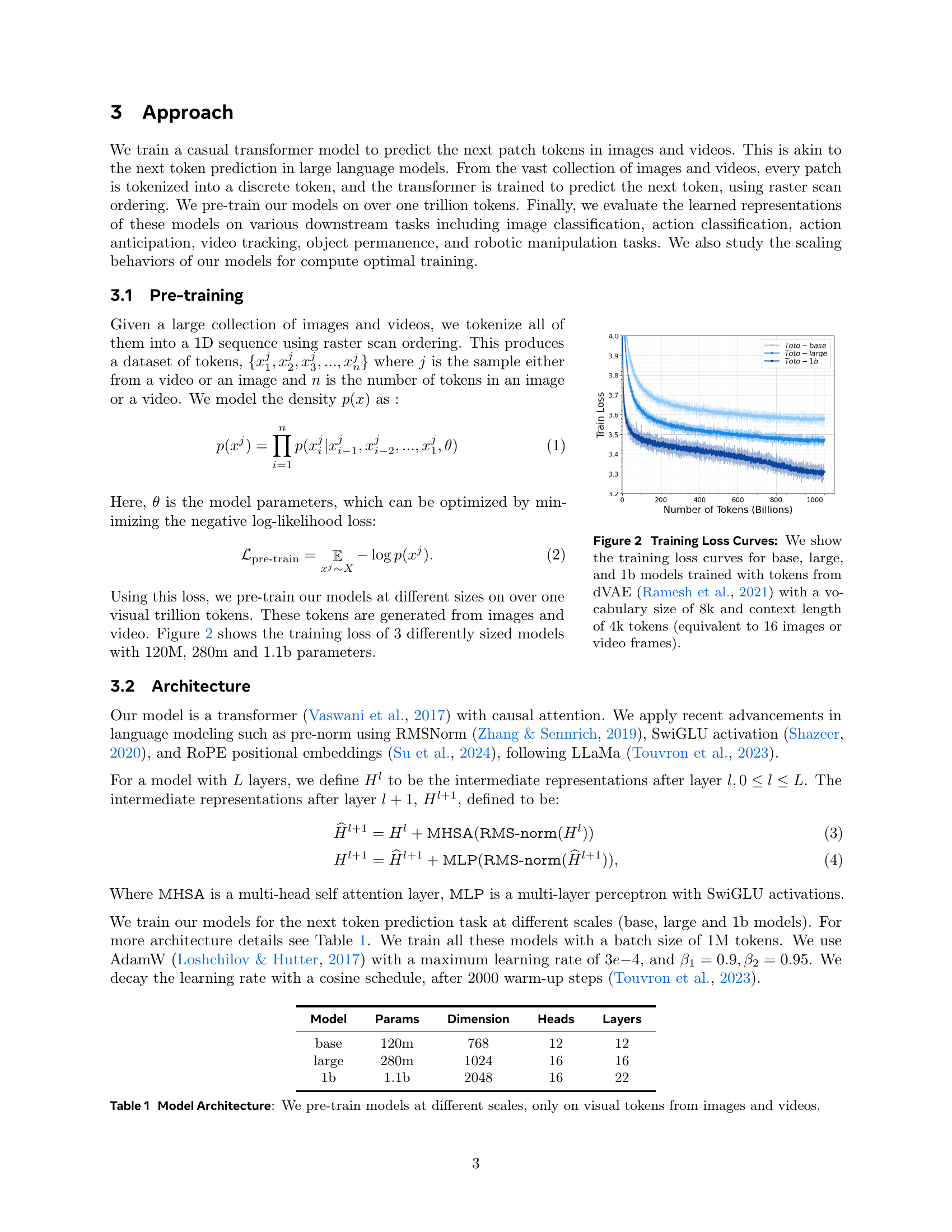
| Model | Params | Dimension | Heads | Layers |
|---|---|---|---|---|
| base | 120m | 768 | 12 | 12 |
| large | 280m | 1024 | 16 | 16 |
| 1b | 1.1b | 2048 | 16 | 22 |
🔼 This table details the architecture of the autoregressive video models (called Toto) used in the study. It shows the model’s parameters (in millions), the dimensionality of the embedding, the number of attention heads, and the number of layers in the transformer network. The table highlights that the models are trained at different scales, with varying numbers of parameters, to analyze the impact of scale on performance. All models are trained solely on visual tokens derived from images and videos.
read the caption
Table 1: Model Architecture: We pre-train models at different scales, only on visual tokens from images and videos.
In-depth insights#
Video Autoregressive#
The concept of “Video Autoregressive” models presents a significant advancement in video processing. It leverages the success of autoregressive models in natural language processing, extending the paradigm to the visual domain. This approach treats a video as a sequence of visual tokens, enabling the prediction of future tokens based on past ones. The key advantage lies in the potential to learn rich, contextualized visual representations directly from raw video data, without explicit supervision. This contrasts with other methods that often rely on pre-trained models or hand-engineered features. Challenges in developing effective video autoregressive models include the inherent complexity of video data (temporal and spatial dependencies), the computational cost of training large models on massive datasets, and the need for efficient tokenization strategies. However, the potential rewards are substantial, including enhanced capabilities for video generation, prediction, understanding, and downstream applications such as action recognition and video forecasting. Future research should focus on addressing the challenges to realize the full potential of this promising technique. The exploration of different tokenization methods and the development of optimized architectures are crucial steps in advancing this field.
Toto Model’s#
The conceptualization and implementation of the “Toto” models represent a significant advancement in autoregressive video pre-training. The core innovation lies in treating videos as sequences of visual tokens, enabling a unified training approach across both images and videos. This approach leverages the power of causal transformers, similar to those used in language modeling, to predict future visual tokens. The architecture incorporates recent advancements like RMSNorm, SwiGLU activation, and ROPE positional embeddings, enhancing efficiency and performance. The models are extensively evaluated across multiple downstream tasks, including image recognition, video classification, and robotics, demonstrating strong generalization capabilities despite minimal inductive biases. A noteworthy aspect is the study of scaling behaviors, revealing similar scaling curves to language models but with a different rate, providing valuable insights into the compute-performance tradeoff. The choice to utilize dVAE tokenization, while not without limitations, demonstrates a conscious decision to prioritize broad applicability and avoids biases inherent in methods that utilize perceptual loss. Overall, the Toto models offer a compelling approach to video understanding, highlighting the potential of autoregressive methods for visual data.
Downstream Tasks#
The evaluation of autoregressive video models on downstream tasks is crucial for demonstrating their practical utility and generalizability. The paper investigates several tasks, including image and video recognition (ImageNet, Kinetics-400), video forecasting (Ego4D), semi-supervised tracking (DAVIS), object permanence (CATER), and robotics. The choice of these tasks reflects a comprehensive assessment of various capabilities that extend beyond simple visual recognition, encompassing higher-level understanding and complex interaction with the environment. The strong performance observed across these diverse downstream tasks strongly supports the effectiveness of the autoregressive pre-training methodology. Furthermore, the similar scaling trends observed in language and vision models, albeit with a different scaling rate, suggest a deeper underlying relationship between these seemingly disparate modalities. The results provide compelling evidence for the potential of autoregressive pre-training to unlock powerful video representations suitable for various real-world applications, paving the way for further advancements in video understanding.
Scaling Behaviors#
The scaling behaviors analysis within a large language model (LLM) or a vision model is crucial for understanding its performance capabilities and resource requirements. This section would likely explore how the model’s performance changes as its size (number of parameters) and compute resources (training time, FLOPs) are scaled up. Key aspects would include identifying potential scaling laws, which are mathematical relationships describing the improvement in performance as a function of increased scale. The authors might compare these scaling laws to those observed in other models, particularly LLMs, to understand the unique scaling characteristics of their model. Analyzing the rate of diminishing returns is important; simply increasing scale doesn’t guarantee proportional improvements. A key insight is whether the model’s scaling behavior shows an optimal ‘sweet spot’ beyond which further scaling yields limited gains. The analysis should present quantitative results showing the trade-offs between performance gains and computational costs, allowing researchers to make informed decisions about model design and resource allocation. The existence of a ‘compute optimal scaling law’ would be a significant finding, providing a valuable guideline for future model development.
Future Work#
Future research directions stemming from this autoregressive video pre-training work could focus on several key areas. Addressing the limitations of internet-scale video data is crucial; future work should explore methods to mitigate the negative impacts of data quality and diversity issues. Developing a more robust and universal visual tokenizer is also important, moving beyond current limitations and improving both representation and generation quality. Investigating alternative training paradigms that reduce redundancy in video frame data may significantly enhance learned representations. The current study primarily focuses on ImageNet classification; further investigation into the effectiveness of the proposed approach on a wider range of tasks, including dense prediction, fine-grained recognition, and more complex temporal dynamics, is necessary. Finally, scaling experiments highlight that visual next-token prediction models scale, but slower than language models; exploring this difference through deeper analysis and potentially novel architectural design choices would be valuable.
More visual insights#
More on figures

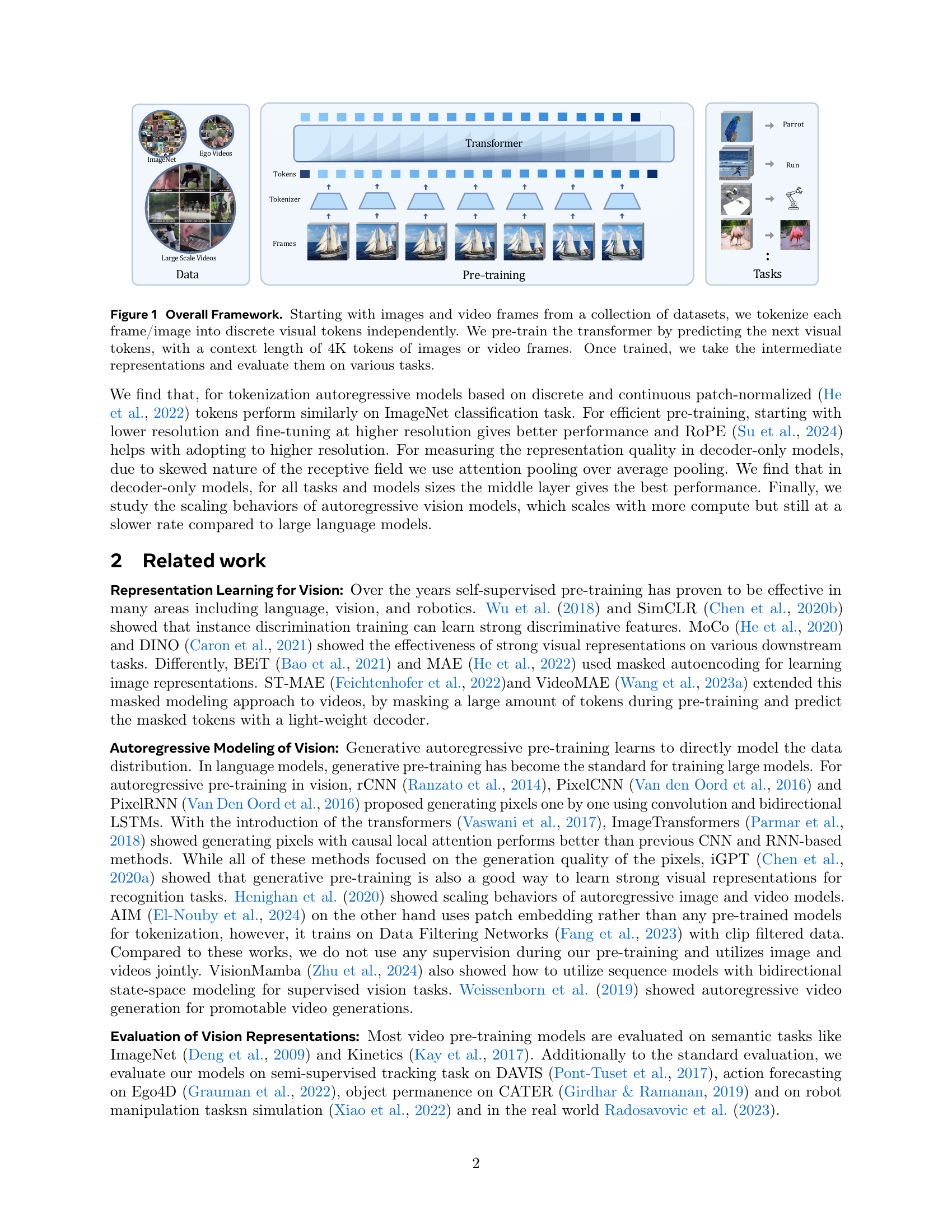
🔼 This figure displays the training loss curves for three different sized autoregressive video models (Toto): a base model, a large model, and a 1 billion parameter model. The models were trained using visual tokens generated by a discrete variational autoencoder (dVAE) with a vocabulary size of 8,000 tokens. Each model’s training data consisted of sequences of 4,000 tokens, which equates to roughly 16 images or video frames in length. The graph shows how the training loss decreases as the number of training tokens increases for each model, indicating the models’ learning progress during pre-training.
read the caption
Figure 2: Training Loss Curves: We show the training loss curves for base, large, and 1b models trained with tokens from dVAE (Ramesh et al., 2021) with a vocabulary size of 8k and context length of 4k tokens (equivalent to 16 images or video frames).

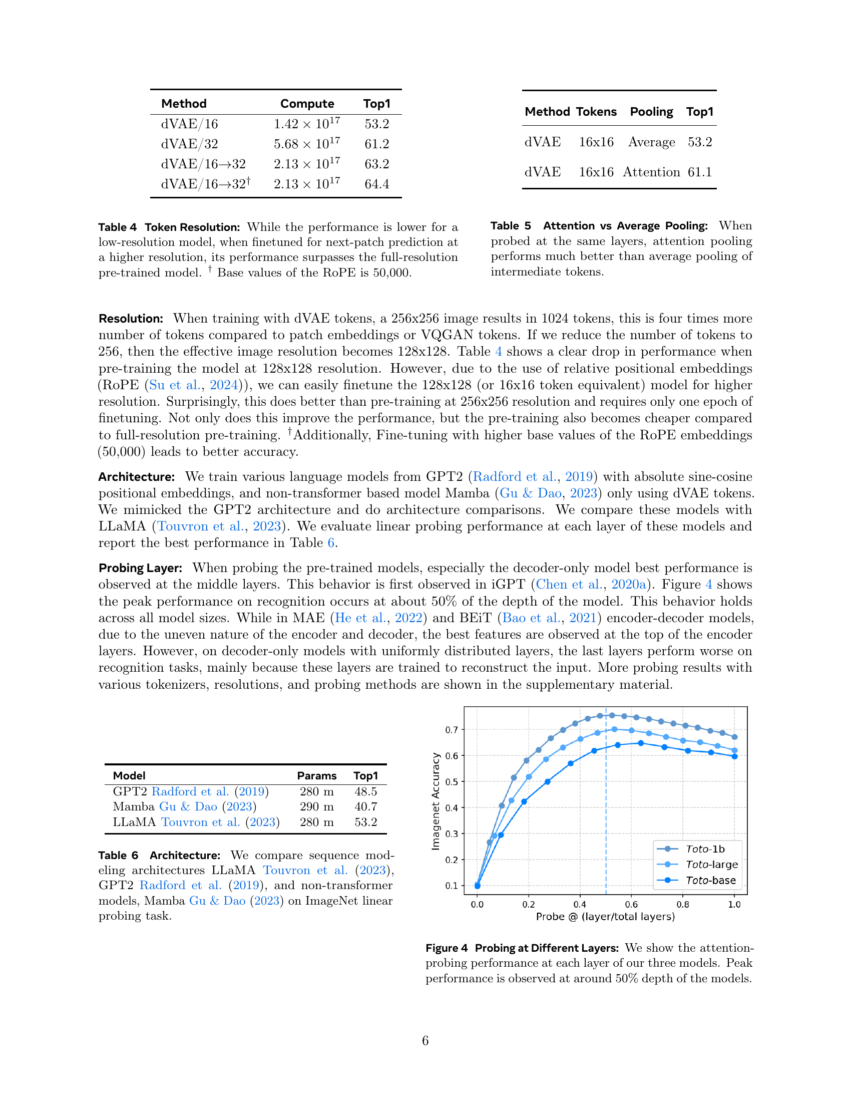
🔼 Figure 3 presents a comparison of the token distributions generated by three different tokenizers: dVAE, VQGAN-1k, and VQGAN-16k. The histograms illustrate the frequency of each unique visual token (1-gram) across the ImageNet validation set. The key observation is the difference in token coverage. dVAE exhibits a much more uniform distribution, with a near-complete coverage of its vocabulary. In contrast, both VQGAN-1k and VQGAN-16k show a significantly less uniform distribution, indicating that a substantial portion of their token vocabularies are underutilized in representing the ImageNet data. This implies that dVAE’s tokenizer may provide more comprehensive coverage of visual features compared to VQGAN.
read the caption
Figure 3: 1-gram Distribution of Various Tokens: This Figure shows the distribution of 1-gram tokens of various tokenizers (dVAE (Ramesh et al., 2021), VQGAN-1k, VQGAN-16k (Esser et al., 2020)) on Imagenet validation set. Note that, dVAE has almost full convergence of the tokens while VQGAN has less than 50% coverage of the tokens.

🔼 This table presents the results of an experiment comparing the performance of autoregressive video models trained at different resolutions. The models were initially trained at either low (128x128) or high (256x256) resolution using discrete visual tokens. The key finding is that even though the low-resolution model initially performed worse, fine-tuning it for next-patch prediction at a higher (256x256) resolution resulted in superior performance compared to the model that was trained directly at the high resolution. This highlights the benefit of starting with lower-resolution training and then subsequently fine-tuning at higher resolution, potentially reducing computational cost without compromising performance. The base value for the Rotary Positional Embeddings (ROPE) was set to 50,000 during training.
read the caption
Table 4: Token Resolution: While the performance is lower for a low-resolution model, when finetuned for next-patch prediction at a higher resolution, its performance surpasses the full-resolution pre-trained model. ††{}^{\text{\textdagger}}start_FLOATSUPERSCRIPT † end_FLOATSUPERSCRIPT Base values of the RoPE is 50,000.

🔼 This table compares the performance of attention pooling and average pooling when extracting features from intermediate layers of a pre-trained model for downstream tasks. It shows that attention pooling, which weights tokens based on their importance, significantly outperforms average pooling, which treats all tokens equally.
read the caption
Table 5: Attention vs Average Pooling: When probed at the same layers, attention pooling performs much better than average pooling of intermediate tokens.

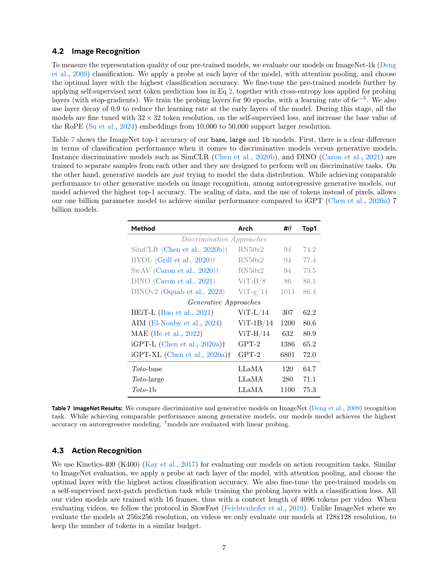
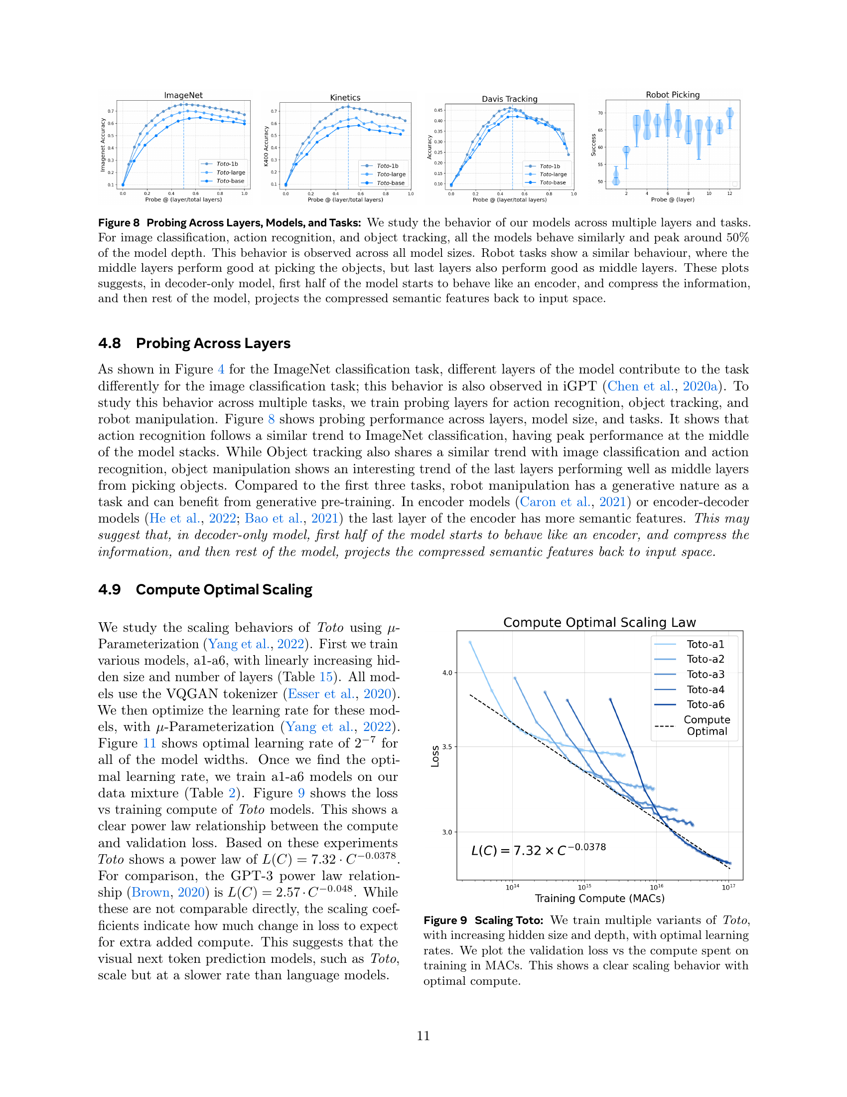
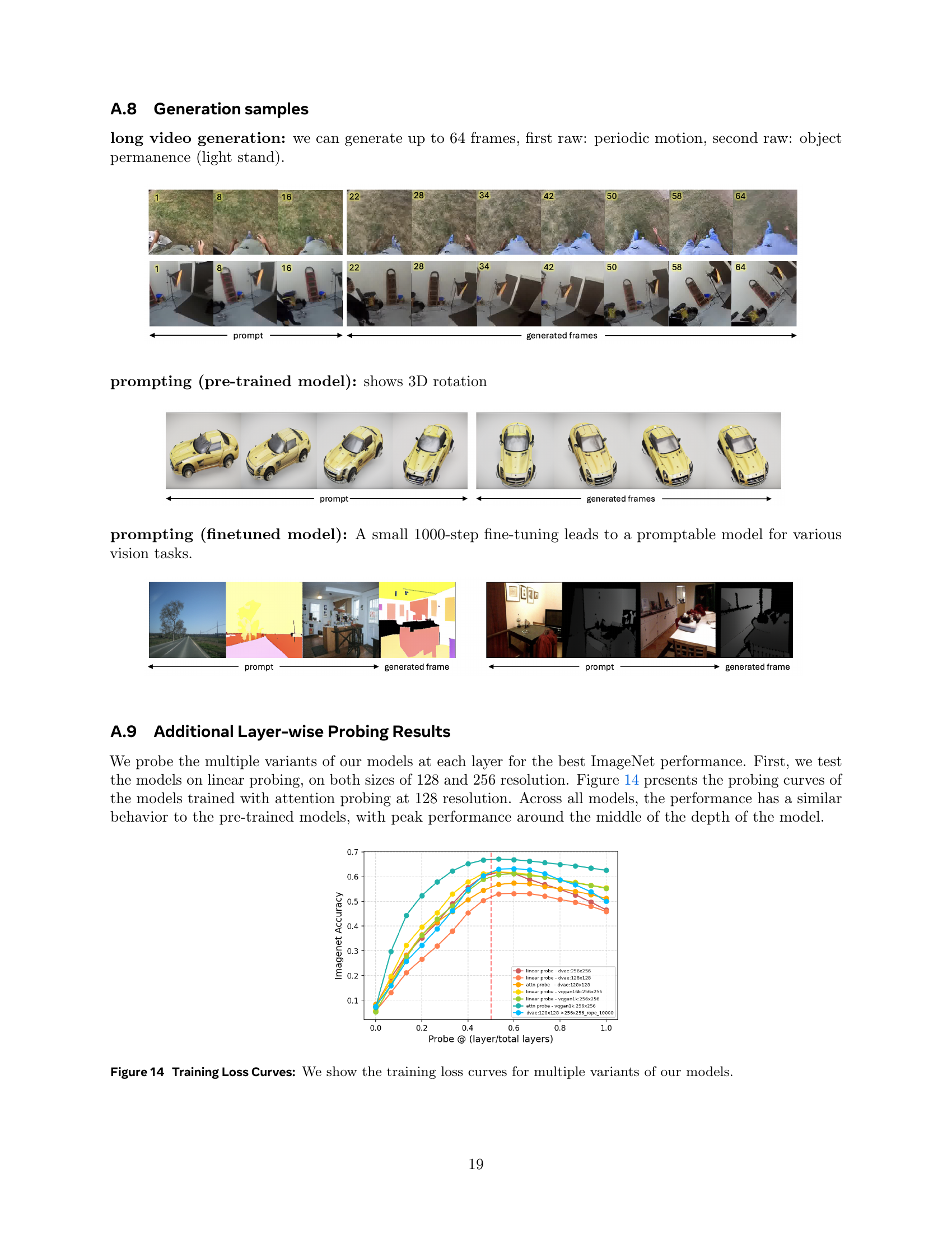
🔼 This figure visualizes the results of an experiment evaluating the performance of different layers within three autoregressive video models (Toto-base, Toto-large, and Toto-1b) on the ImageNet image classification task. The x-axis represents the relative layer depth within each model (0.0 representing the first layer and 1.0 the last), and the y-axis shows the classification accuracy achieved using attention pooling at each layer. The plot demonstrates that for all three models, the highest accuracy is achieved at approximately the 50% mark of the total layer depth, indicating that the most informative features for this task are located in the middle layers of the network. The observation of peak performance in middle layers across different model scales suggests an optimal depth for capturing both local and global contextual information.
read the caption
Figure 4: Probing at Different Layers: We show the attention-probing performance at each layer of our three models. Peak performance is observed at around 50% depth of the models.

🔼 This figure demonstrates semi-supervised video object tracking using the Toto-large model. Following the methodology outlined in Jabri et al. (2020), the process begins with a ground truth (GT) segmentation mask. The model then leverages its learned feature representations to propagate these labels forward in time. The results showcase the model’s ability to maintain accurate tracking across a sequence of 60 frames, highlighting the effectiveness of the model’s features even without explicit supervision in the tracking task.
read the caption
Figure 5: Semi-Supervised Tracking: We follow the protocol in STC (Jabri et al., 2020), start with the GT segmentation mask, and propagate the labels using the features computed by Toto-large. The mask was propagated up to 60 frames without losing much information.

🔼 This figure shows the mean success rate over training steps for a Franka robot performing a pick task. The success rate is plotted against the number of training steps. Two models, Toto-base and MVP-base, are compared, demonstrating that Toto-base learns the task faster than MVP-base.
read the caption
(a) Franka Pick

🔼 This figure is a plot showing the mean success rate over training steps for a Kuka Pick task in a robot manipulation experiment using reinforcement learning. The plot compares the performance of a Toto-base model against a MVP-base model. The x-axis represents the number of training steps, and the y-axis represents the mean success rate. The plot visually demonstrates the learning progress of each model on this specific robotic task.
read the caption
(b) Kuka Pick

🔼 This figure shows the results of a robot manipulation experiment using reinforcement learning. Specifically, it displays the mean success rate over training steps for a Franka robot performing a cabinet-opening task. The graph likely compares the performance of the Toto-base model to a baseline model (potentially MAE-base) to illustrate the improved learning efficiency and success rate achieved with the pre-trained Toto model.
read the caption
(c) Franka Cabinet

🔼 The figure shows the mean success rate over training steps for a Kuka Cabinet task in robot manipulation experiments using reinforcement learning. It compares the performance of a Toto-base model against a MAE-base model, illustrating the Toto model’s faster learning and improved sample efficiency.
read the caption
(d) Kuka Cabinet

🔼 Figure 6 presents a comparison of the learning performance between MAE-base (a previously published model) and Toto-base (the model introduced in this paper) on robot manipulation tasks within a simulated environment. The experiments follow the methodology outlined in Xiao et al. (2022). The figure displays the mean success rate achieved by each model across different training steps for four tasks: Franka-Pick, Kuka-Pick, Franka-Cabinet, and Kuka-Cabinet. Two different robot arms (Franka and Kuka) are involved. The results demonstrate that Toto-base learns these robotic manipulation tasks more efficiently (i.e., in fewer training steps) than MAE-base across both robot types and all four tasks.
read the caption
Figure 6: Robot Manipulation with Reinforcement Learning: We compare MAE-base (Radosavovic et al., 2022) with Toto-base pre-trained models in simulation following Xiao et al. (2022). We evaluate each model the mean success rate over training steps. Toto was able to learn these tasks faster than MAE, across two robots and two tasks.

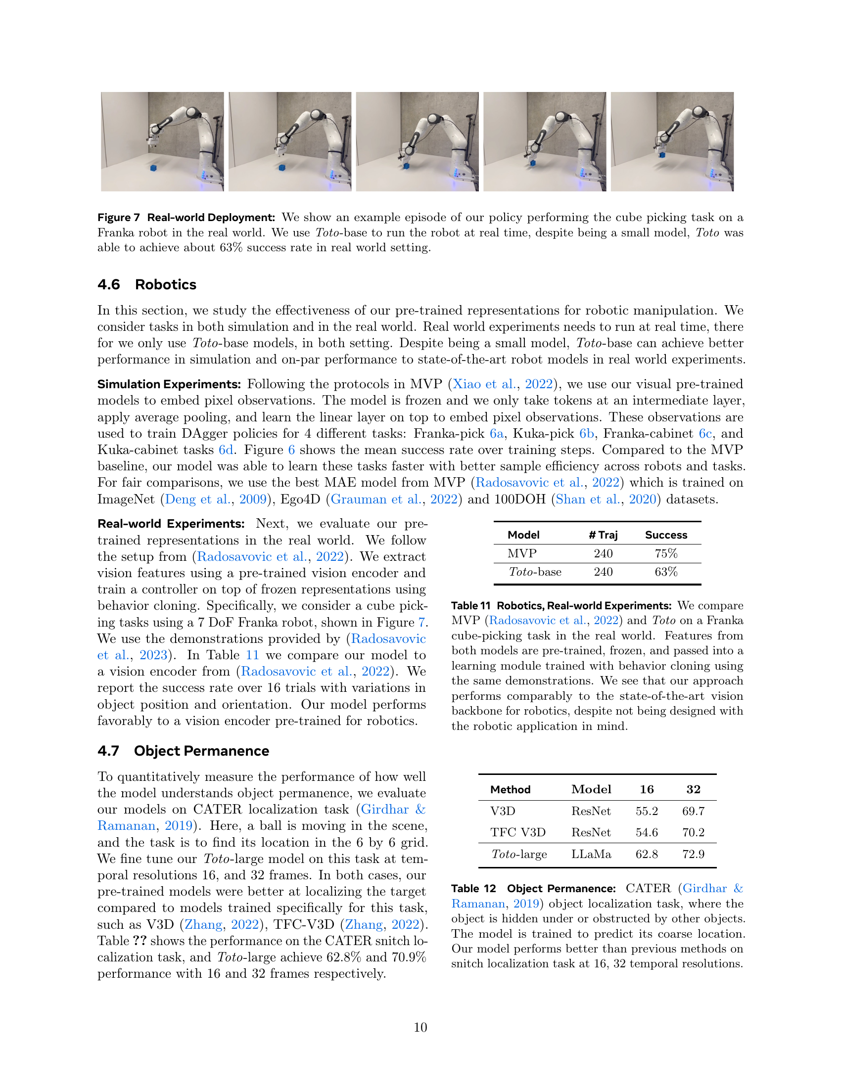
🔼 This figure showcases a real-world application of the Toto-base model in a robotic manipulation task. Specifically, it shows an example sequence of a Franka robot performing a cube-picking task. The key takeaway is that despite its relatively small size, the Toto-base model enables real-time control of the robot, achieving a success rate of approximately 63% in this challenging real-world environment. This demonstrates the effectiveness and efficiency of the autoregressive pre-training approach used in developing the Toto models for real-world robotic applications.
read the caption
Figure 7: Real-world Deployment: We show an example episode of our policy performing the cube picking task on a Franka robot in the real world. We use Toto-base to run the robot at real time, despite being a small model, Toto was able to achieve about 63% success rate in real world setting.

🔼 This figure visualizes the performance of different layers within the model across various tasks (ImageNet classification, Kinetics action recognition, DAVIS object tracking, and robot manipulation). For ImageNet, Kinetics, and DAVIS, peak performance is consistently observed around the middle layers (approximately 50% of the total depth), regardless of model size. Interestingly, robot manipulation tasks show a different pattern, with both middle and later layers exhibiting strong performance. This suggests that in decoder-only models, the initial layers function as an encoder, compressing information before the later layers project the compressed features back into the input space. The results highlight the distinct roles of different layers and their varying suitability across diverse tasks.
read the caption
Figure 8: Probing Across Layers, Models, and Tasks: We study the behavior of our models across multiple layers and tasks. For image classification, action recognition, and object tracking, all the models behave similarly and peak around 50% of the model depth. This behavior is observed across all model sizes. Robot tasks show a similar behaviour, where the middle layers perform good at picking the objects, but last layers also perform good as middle layers. These plots suggests, in decoder-only model, first half of the model starts to behave like an encoder, and compress the information, and then rest of the model, projects the compressed semantic features back to input space.

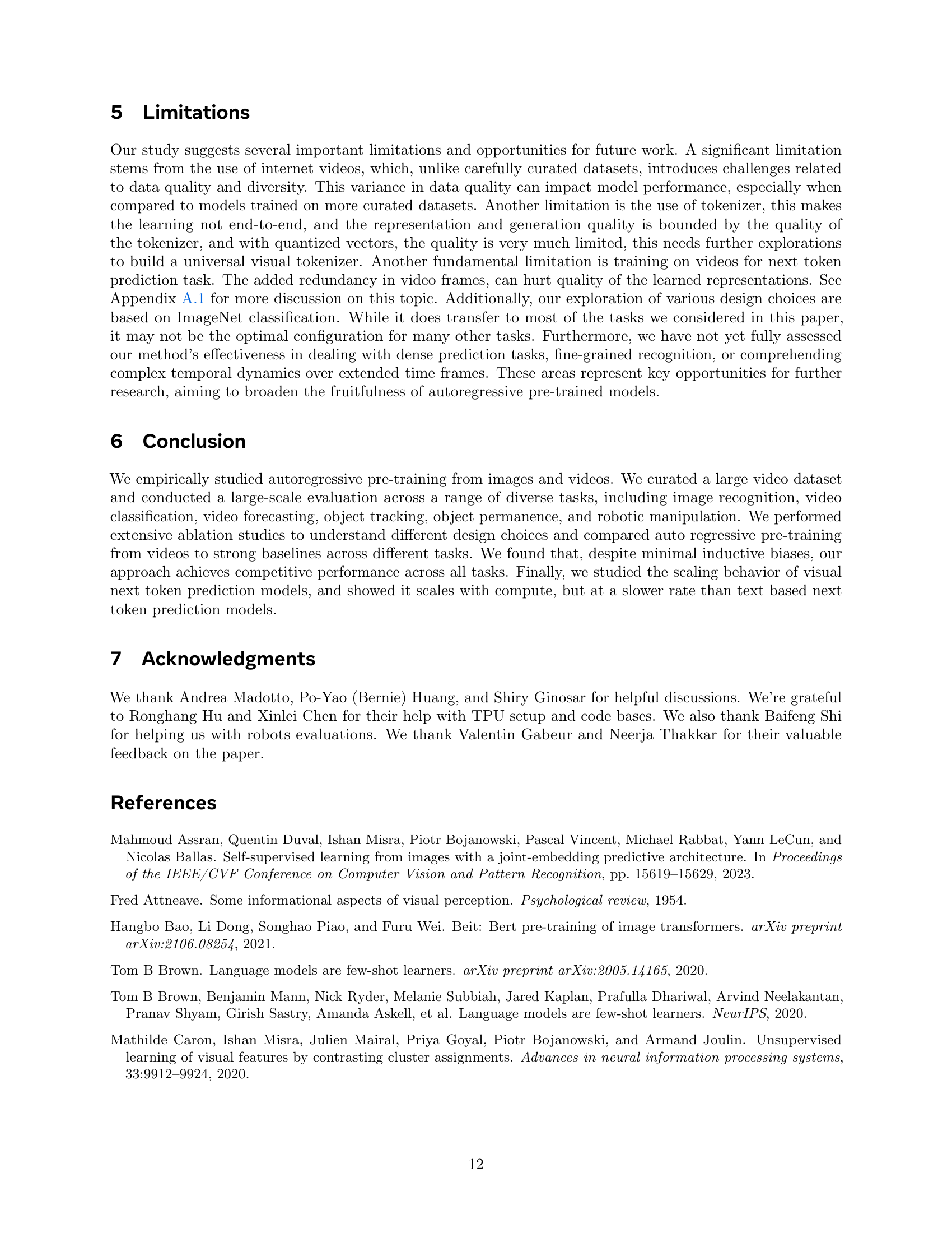
🔼 This figure demonstrates the scaling behavior of the Toto model family. Multiple versions of the model were trained with varying hidden sizes and depths; for each, the optimal learning rate was determined. The plot shows the validation loss against the total compute (measured in Multiply-Accumulate operations, or MACs) used during training. The graph clearly illustrates how increasing compute resources leads to lower validation loss, demonstrating the scaling efficiency of the models.
read the caption
Figure 9: Scaling Toto: We train multiple variants of Toto, with increasing hidden size and depth, with optimal learning rates. We plot the validation loss vs the compute spent on training in MACs. This shows a clear scaling behavior with optimal compute.

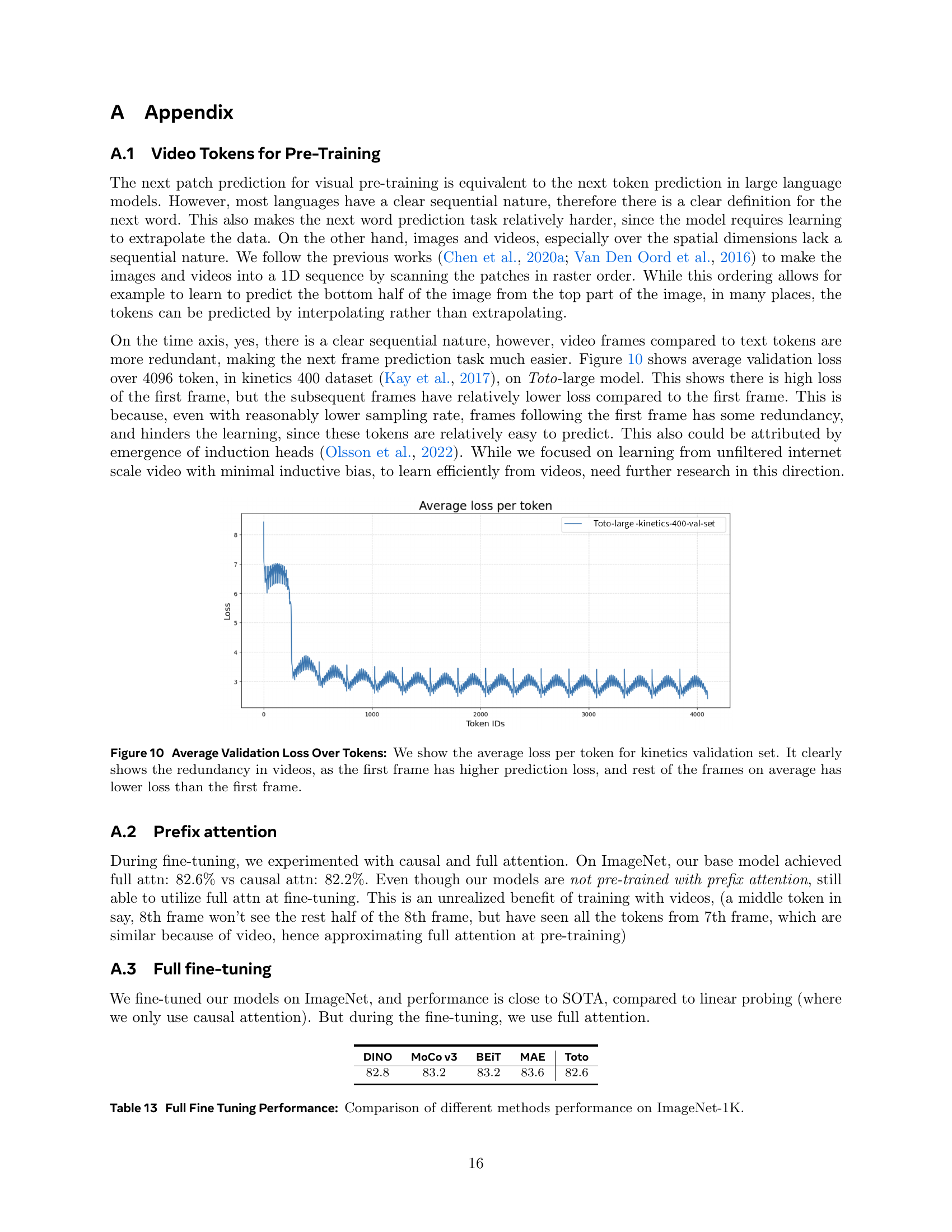
🔼 Figure 10 illustrates the average validation loss per token calculated on the Kinetics-400 validation dataset. The graph reveals a pattern of redundancy in video data. The first frame in a video sequence exhibits a significantly higher average loss than subsequent frames. This is because the model has to learn the overall content and context of the video from the very first frame, facing a greater challenge in prediction. In contrast, later frames benefit from the previously established context and temporal relationships, making prediction easier. The lower loss for subsequent frames demonstrates the inherent redundancy present in videos. This observation suggests that the model can more easily predict later frames due to the established context of prior frames. This effect highlights a key difference between video data and textual data, where the sequential nature of language makes each word more dependent on the context that precedes it.
read the caption
Figure 10: Average Validation Loss Over Tokens: We show the average loss per token for kinetics validation set. It clearly shows the redundancy in videos, as the first frame has higher prediction loss, and rest of the frames on average has lower loss than the first frame.

🔼 This table details the specifications of six different variations of the Toto model. These variations are created by systematically scaling up the model’s hidden dimension and number of layers, while maintaining a constant number of attention heads. This scaling approach follows the methods described by Yang et al. (2022) and Touvron et al. (2023), allowing for a systematic exploration of the effects of model size on performance and resource utilization.
read the caption
Table 15: Toto Varients: We scale Toto models by increasing hidden dimension and number of layers linearly while keeping number of heads constant following (Yang et al., 2022; Touvron et al., 2023).

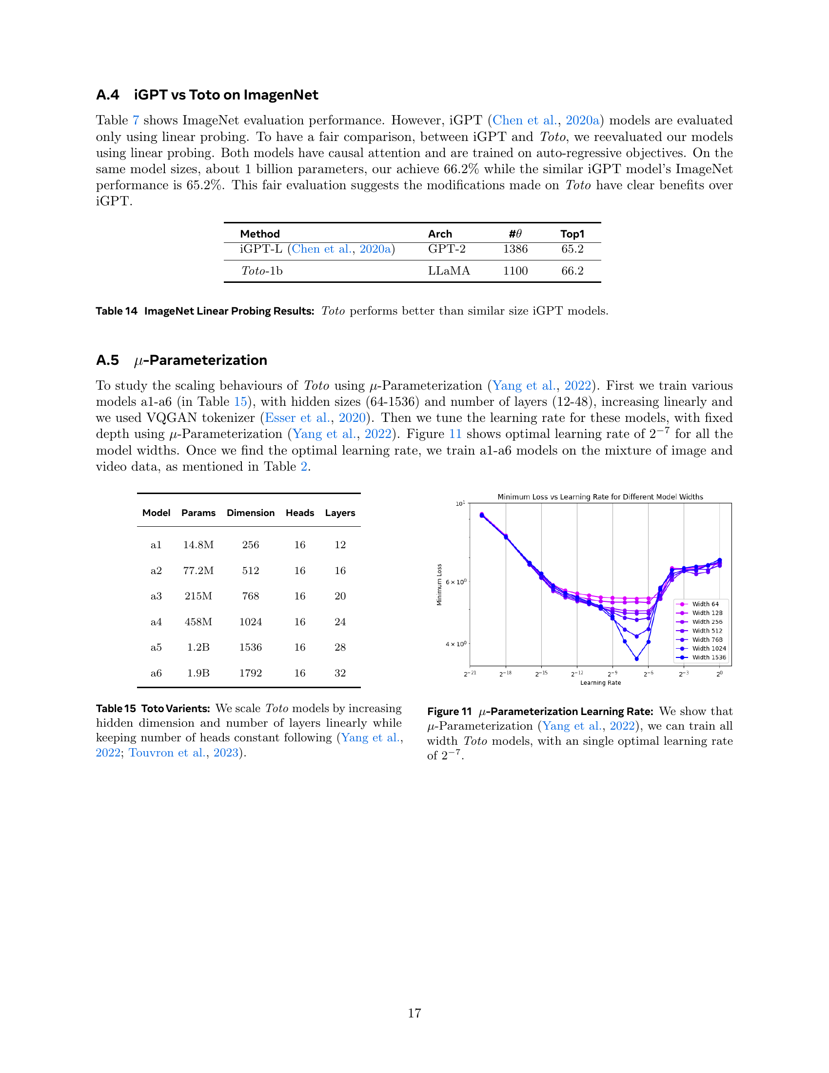
🔼 This figure demonstrates the effectiveness of μ-parameterization in finding a single optimal learning rate for various Toto model widths. The x-axis represents the learning rate, ranging from 2-2 to 2-7, while the y-axis shows the minimum validation loss achieved for each model width. Each curve represents a different model width, and it shows that despite the differing model complexities, a single optimal learning rate range (2-2 to 2-7) minimizes validation loss across all model sizes. This highlights the utility of μ-parameterization in simplifying the training process for various model scales.
read the caption
Figure 11: μ𝜇\muitalic_μ-Parameterization Learning Rate: We show that μ𝜇\muitalic_μ-Parameterization (Yang et al., 2022), we can train all width Toto models, with an single optimal learning rate of 2−7superscript272^{-7}2 start_POSTSUPERSCRIPT - 7 end_POSTSUPERSCRIPT.

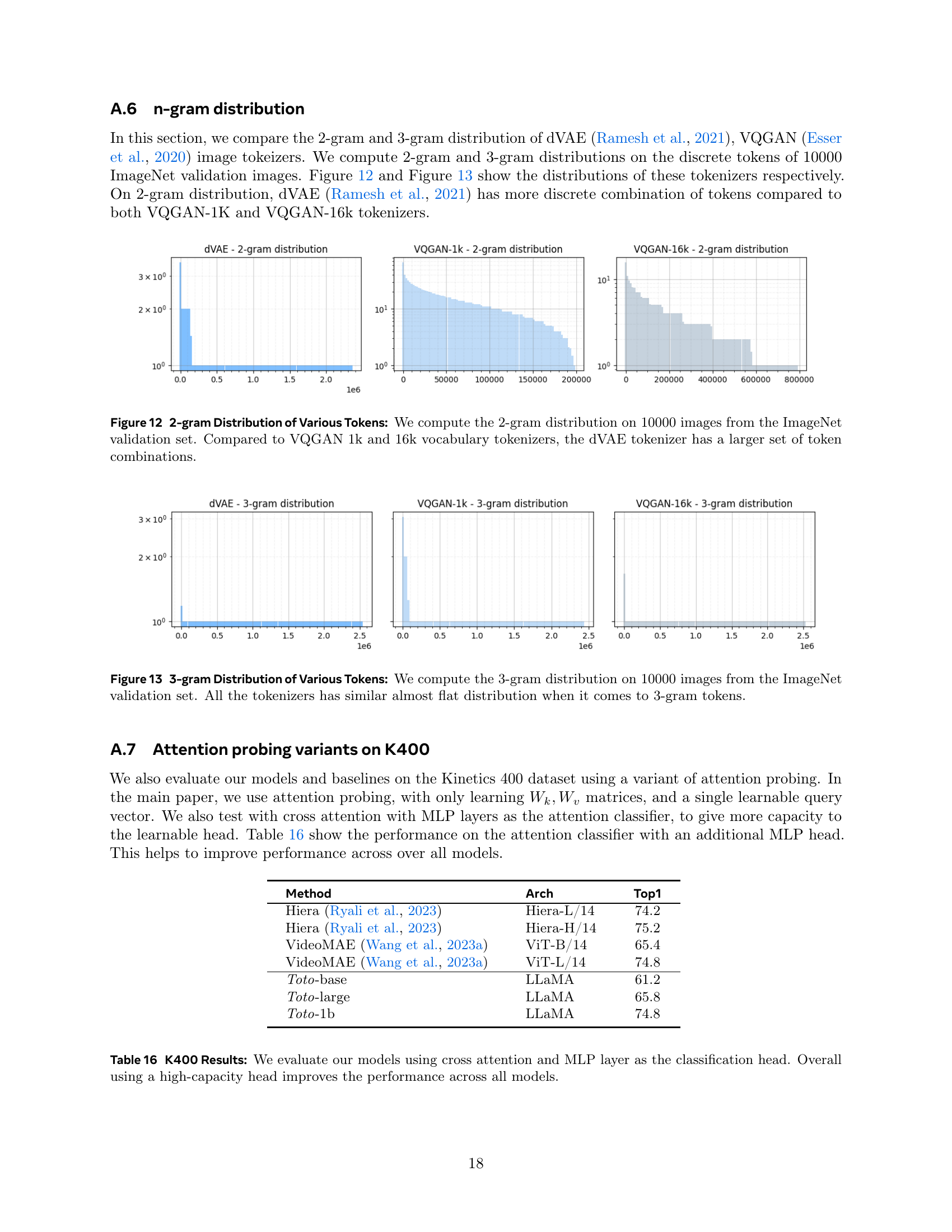
🔼 This figure compares the 2-gram distributions of visual tokens generated by three different tokenizers: dVAE, VQGAN-1k, and VQGAN-16k. The analysis is performed on 10,000 images from the ImageNet validation set. The histograms display the frequency of each unique pair of consecutive tokens (2-grams). The figure illustrates that the dVAE tokenizer produces a significantly broader range of 2-gram combinations compared to both variants of the VQGAN tokenizer, suggesting a more diverse and richer representation of visual information.
read the caption
Figure 12: 2-gram Distribution of Various Tokens: We compute the 2-gram distribution on 10000 images from the ImageNet validation set. Compared to VQGAN 1k and 16k vocabulary tokenizers, the dVAE tokenizer has a larger set of token combinations.

🔼 Figure 13 compares the distribution of 3-grams for different visual tokenizers (dVAE, VQGAN-1k, and VQGAN-16k) trained on 10,000 images from the ImageNet validation set. The 3-gram distributions show that all three tokenizers have similar distributions, largely flat, indicating a lack of strong sequential patterns or dependencies between tokens at this level.
read the caption
Figure 13: 3-gram Distribution of Various Tokens: We compute the 3-gram distribution on 10000 images from the ImageNet validation set. All the tokenizers has similar almost flat distribution when it comes to 3-gram tokens.
More on tables
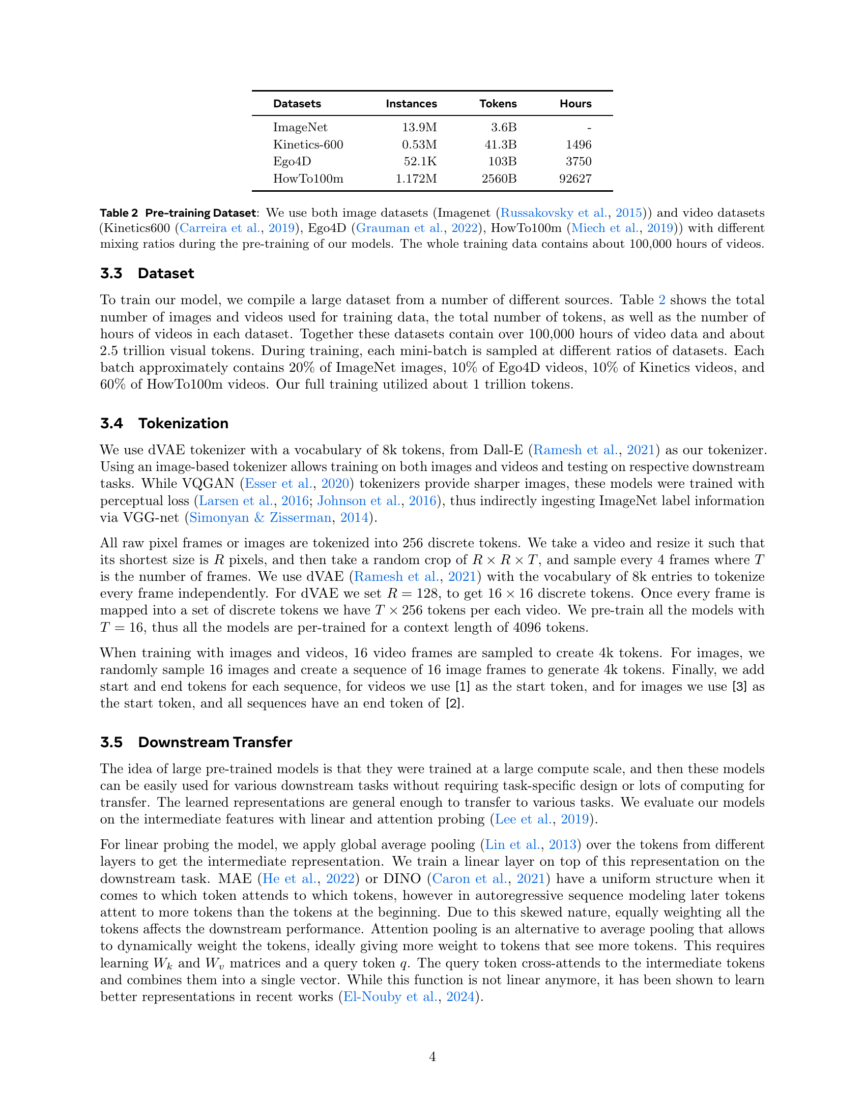
| Datasets | Instances | Tokens | Hours |
|---|---|---|---|
| ImageNet | 13.9M | 3.6B | - |
| Kinetics-600 | 0.53M | 41.3B | 1496 |
| Ego4D | 52.1K | 103B | 3750 |
| HowTo100m | 1.172M | 2560B | 92627 |
🔼 This table details the datasets used for pre-training the video models. It lists four datasets: ImageNet (a large image dataset), Kinetics-600 (a dataset of short video clips with action labels), Ego4D (a large-scale egocentric video dataset), and HowTo100M (a dataset of how-to videos with text descriptions). For each dataset, the table provides the number of instances (images or videos), the total number of visual tokens generated from them, and the approximate number of hours of video content. Note that the datasets were combined in different ratios during training, and the total training data comprised over 100,000 hours of video and roughly 1 trillion tokens. This demonstrates the massive scale of data used to pre-train the autoregressive video models.
read the caption
Table 2: Pre-training Dataset: We use both image datasets (Imagenet (Russakovsky et al., 2015)) and video datasets (Kinetics600 (Carreira et al., 2019), Ego4D (Grauman et al., 2022), HowTo100m (Miech et al., 2019)) with different mixing ratios during the pre-training of our models. The whole training data contains about 100,000 hours of videos.
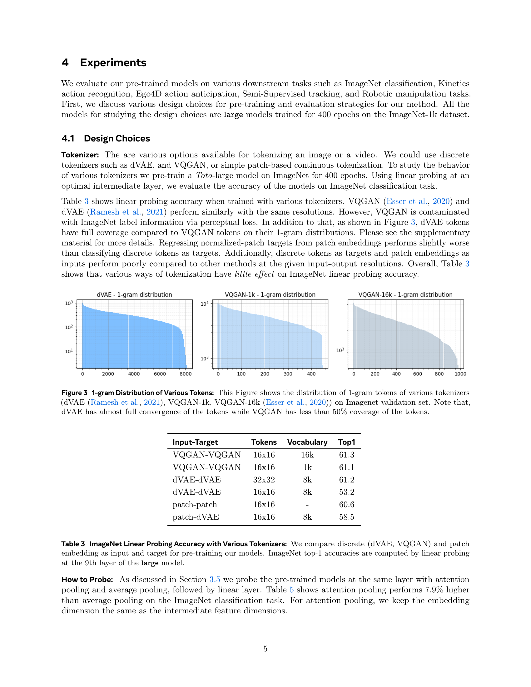
| Input-Target | Tokens | Vocabulary | Top1 |
|---|---|---|---|
| VQGAN-VQGAN | 16x16 | 16k | 61.3 |
| VQGAN-VQGAN | 16x16 | 1k | 61.1 |
| dVAE-dVAE | 32x32 | 8k | 61.2 |
| dVAE-dVAE | 16x16 | 8k | 53.2 |
| patch-patch | 16x16 | - | 60.6 |
| patch-dVAE | 16x16 | 8k | 58.5 |
🔼 This table presents the results of an experiment comparing different tokenization methods for training a vision transformer model. The goal was to determine the impact of various tokenization techniques on the model’s performance on ImageNet image classification. The experiment used three types of tokenizers: discrete tokenizers (dVAE and VQGAN), and a patch-based continuous tokenizer. For each tokenizer, the model was pre-trained, then its performance on ImageNet was evaluated using linear probing on the 9th layer of a ’large’ model. The table shows the top-1 accuracy achieved for each combination of input/target tokenizer and indicates that the choice of tokenizer has a relatively minor impact on performance.
read the caption
Table 3: ImageNet Linear Probing Accuracy with Various Tokenizers: We compare discrete (dVAE, VQGAN) and patch embedding as input and target for pre-training our models. ImageNet top-1 accuracies are computed by linear probing at the 9th layer of the large model.
| Method | Compute | Top1 |
|---|---|---|
| dVAE/16 | 1.42 × 10¹⁷ | 53.2 |
| dVAE/32 | 5.68 × 10¹⁷ | 61.2 |
| dVAE/16 → 32 | 2.13 × 10¹⁷ | 63.2 |
| dVAE/16 → 32† | 2.13 × 10¹⁷ | 64.4 |
🔼 This table compares the performance of different neural network architectures on the ImageNet image classification task using a linear probing method. The architectures compared include the LLaMA transformer model, the GPT-2 transformer model, and the non-transformer Mamba model. The table shows the number of parameters in each model and its top-1 accuracy on ImageNet after linear probing. This allows for a comparison of the effectiveness of different architectural designs for visual representation learning.
read the caption
Table 6: Architecture: We compare sequence modeling architectures LLaMA Touvron et al. (2023), GPT2 Radford et al. (2019), and non-transformer models, Mamba Gu & Dao (2023) on ImageNet linear probing task.
| Method | Tokens | Pooling | Top1 |
|---|---|---|---|
| dVAE | 16x16 | Average | 53.2 |
| dVAE | 16x16 | Attention | 61.1 |
🔼 Table 7 presents the ImageNet classification results, comparing various discriminative and generative vision models. The table highlights the top-1 accuracy achieved by each model. It’s particularly noteworthy that the proposed Toto models achieve the highest accuracy among the autoregressive generative models, demonstrating the effectiveness of the autoregressive pre-training approach. Models marked with † were evaluated using linear probing, meaning their performance was assessed by attaching a simple linear layer on top of the model’s extracted features, without further fine-tuning.
read the caption
Table 7: ImageNet Results: We compare discriminative and generative models on ImageNet (Deng et al., 2009) recognition task. While achieving comparable performance among generative models, our models model achieves the highest accuracy on autoregressive modeling. †models are evaluated with linear probing.
| Model | Params | Top1 |
|---|---|---|
| GPT2 [Radford et al. (2019)] | 280 m | 48.5 |
| Mamba [Gu & Dao (2023)] | 290 m | 40.7 |
| LLaMA [Touvron et al. (2023)] | 280 m | 53.2 |
🔼 Table 8 presents a comparison of various models’ performance on the Kinetics-400 action recognition dataset. It contrasts discriminative and generative approaches, highlighting the performance of the proposed ‘Toto’ models. A key takeaway is that while comparable to other generative models, Toto demonstrates competitive results, especially notable as the first to achieve such performance using an autoregressive pre-training method. Furthermore, the table shows that the performance of Toto models scales positively with model size.
read the caption
Table 8: K400 Results: We compare discriminative and generative models on Kinetics-400 (Kay et al., 2017) action recognition task. While achieving comparable performance among generative models, our models are the first to show the competitive performance on K400 with autoregressive pre-training, and shows scaling with large model sizes.
| Method | Arch | #θ | Top1 |
|---|---|---|---|
| Discriminative Approaches | |||
| SimCLR (Chen et al., 2020b)† | RN50x2 | 94 | 74.2 |
| BYOL (Grill et al., 2020)† | RN50x2 | 94 | 77.4 |
| SwAV (Caron et al., 2020)† | RN50x2 | 94 | 73.5 |
| DINO (Caron et al., 2021) | ViT-B/8 | 86 | 80.1 |
| DINOv2 (Oquab et al., 2023) | ViT-g/14 | 1011 | 86.4 |
| Generative Approaches | |||
| BEiT-L (Bao et al., 2021) | ViT-L/14 | 307 | 62.2 |
| AIM (El-Nouby et al., 2024) | ViT-1B/14 | 1200 | 80.6 |
| MAE (He et al., 2022) | ViT-H/14 | 632 | 80.9 |
| iGPT-L (Chen et al., 2020a)† | GPT-2 | 1386 | 65.2 |
| iGPT-XL (Chen et al., 2020a)† | GPT-2 | 6801 | 72.0 |
| Toto-base | LLaMA | 120 | 64.7 |
| Toto-large | LLaMA | 280 | 71.1 |
| Toto-1b | LLaMA | 1100 | 75.3 |
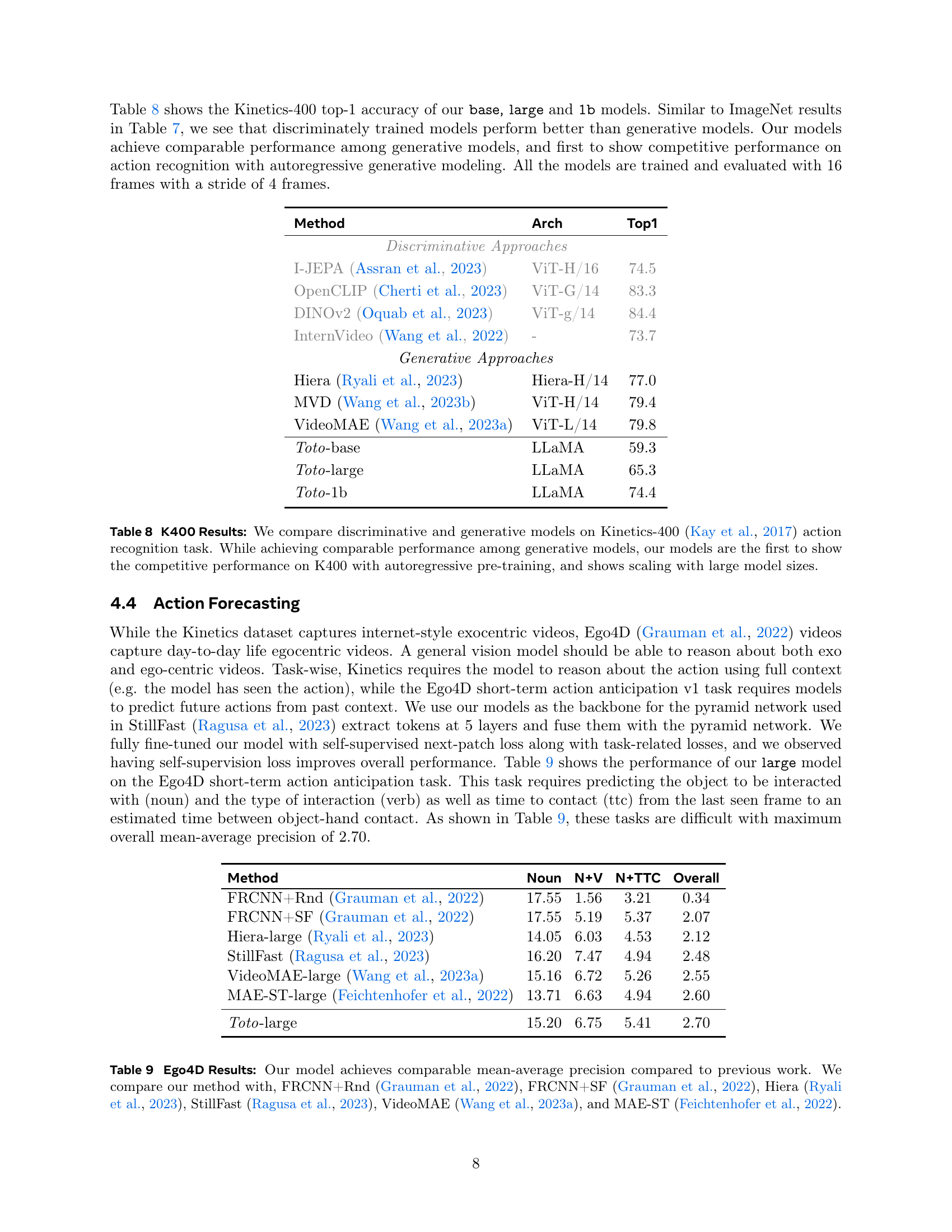
🔼 This table presents a comparison of the performance of different methods on the Ego4D action anticipation dataset. The metric used is mean average precision (mAP), broken down into three components: noun prediction, noun+verb prediction, and noun+verb+time-to-contact prediction. The table compares the proposed ‘Toto-large’ model to several state-of-the-art methods, including FRCNN with random and StillFast baselines from the original Ego4D paper, as well as more recently published models like Hiera and VideoMAE. This allows for an evaluation of the proposed model’s performance relative to existing approaches on this challenging video prediction task.
read the caption
Table 9: Ego4D Results: Our model achieves comparable mean-average precision compared to previous work. We compare our method with, FRCNN+Rnd (Grauman et al., 2022), FRCNN+SF (Grauman et al., 2022), Hiera (Ryali et al., 2023), StillFast (Ragusa et al., 2023), VideoMAE (Wang et al., 2023a), and MAE-ST (Feichtenhofer et al., 2022).
| Method | Arch | Top1 |
|---|---|---|
| Discriminative Approaches | ||
| I-JEPA (Assran et al., 2023) | ViT-H/16 | 74.5 |
| OpenCLIP (Cherti et al., 2023) | ViT-G/14 | 83.3 |
| DINOv2 (Oquab et al., 2023) | ViT-g/14 | 84.4 |
| InternVideo (Wang et al., 2022) | - | 73.7 |
| Generative Approaches | ||
| Hiera (Ryali et al., 2023) | Hiera-H/14 | 77.0 |
| MVD (Wang et al., 2023b) | ViT-H/14 | 79.4 |
| VideoMAE (Wang et al., 2023a) | ViT-L/14 | 79.8 |
| Toto-base | LLaMA | 59.3 |
| Toto-large | LLaMA | 65.3 |
| Toto-1b | LLaMA | 74.4 |
🔼 This table presents the results of a video tracking experiment on the DAVIS dataset. Specifically, it shows the performance of different models (Toto-base, Toto-large, Toto-1b, DINO-base, and MAE-base) in terms of J, F, and J&F scores. The J and F scores represent the Jaccard and F1 scores, respectively, which are common metrics for evaluating object segmentation. The J&F score is the average of the J and F scores. Results are reported for different model resolutions (256x8 and 512x8) and patch sizes. The table highlights that the Toto models, particularly the larger models at higher resolution, achieve comparable performance to DINO and even surpasses other methods.
read the caption
Table 10: DAVIS Tracking: We report J, F, and J&F scores at the peak layers of each model. We achieves comparable performance as DINO and at large resolution (512), it outperforms all methods.
| Method | Noun | N+V | N+TTC | Overall |
|---|---|---|---|---|
| FRCNN+Rnd (Grauman et al., 2022) | 17.55 | 1.56 | 3.21 | 0.34 |
| FRCNN+SF (Grauman et al., 2022) | 17.55 | 5.19 | 5.37 | 2.07 |
| Hiera-large (Ryali et al., 2023) | 14.05 | 6.03 | 4.53 | 2.12 |
| StillFast (Ragusa et al., 2023) | 16.20 | 7.47 | 4.94 | 2.48 |
| VideoMAE-large (Wang et al., 2023a) | 15.16 | 6.72 | 5.26 | 2.55 |
| MAE-ST-large (Feichtenhofer et al., 2022) | 13.71 | 6.63 | 4.94 | 2.60 |
| Toto-large | 15.20 | 6.75 | 5.41 | 2.70 |
🔼 This table presents a comparison of the performance of two different methods on a real-world robotic cube-picking task. The methods compared are MVP (a state-of-the-art vision model for robotics) and Toto (the autoregressive video model introduced in this paper). Both models’ visual features were pre-trained and then frozen; these features were fed into a learning module trained using behavior cloning with identical demonstrations for both models. The results show that Toto’s performance is comparable to MVP’s, demonstrating that a model not specifically designed for robotics can still achieve state-of-the-art results when leveraging effective pre-trained visual features.
read the caption
Table 11: Robotics, Real-world Experiments: We compare MVP (Radosavovic et al., 2022) and Toto on a Franka cube-picking task in the real world. Features from both models are pre-trained, frozen, and passed into a learning module trained with behavior cloning using the same demonstrations. We see that our approach performs comparably to the state-of-the-art vision backbone for robotics, despite not being designed with the robotic application in mind.
| Method (Res/Patch) | J&F | J | F |
|---|---|---|---|
| DINO-base (224/8) | 54.3 | 52.5 | 56.1 |
| DINO-base (224/16) | 33.1 | 36.2 | 30.1 |
| MAE-base (224/16) | 31.5 | 34.1 | 28.9 |
| Toto-base (256/8) | 42.0 | 41.2 | 43.1 |
| Toto-large (256/8) | 44.8 | 44.4 | 45.1 |
| Toto-1b (256/8) | 46.1 | 45.8 | 46.4 |
| Toto-large (512/8) | 62.4 | 59.2 | 65.6 |
🔼 This table presents the results of the object permanence task from the CATER dataset (Girdhar & Ramanan, 2019). The task involves predicting the coarse location of an object that is hidden or occluded by other objects in a scene. The table compares the performance of the proposed Toto model against previous methods. Performance is evaluated at two different temporal resolutions (16 and 32 frames), demonstrating the Toto model’s superior performance in object localization even when the object is not directly visible.
read the caption
Table 12: Object Permanence: CATER (Girdhar & Ramanan, 2019) object localization task, where the object is hidden under or obstructed by other objects. The model is trained to predict its coarse location. Our model performs better than previous methods on snitch localization task at 16, 32 temporal resolutions.
| Model | # Traj | Success |
|---|---|---|
| MVP | 240 | 75% |
| Toto-base | 240 | 63% |
🔼 This table presents a comparison of the top-1 accuracy achieved on the ImageNet-1K dataset by several different self-supervised learning methods after full fine-tuning. The methods compared include DINO, MoCoV3, BEIT, MAE, and the Toto model (the model presented in this paper). The results show the top-1 accuracy achieved by each method.
read the caption
Table 13: Full Fine Tuning Performance: Comparison of different methods performance on ImageNet-1K.
| Method | Model | 16 | 32 |
|---|---|---|---|
| V3D | ResNet | 55.2 | 69.7 |
| TFC V3D | ResNet | 54.6 | 70.2 |
| Toto-large | LLaMa | 62.8 | 72.9 |
🔼 This table presents the results of linear probing experiments conducted on the ImageNet dataset, comparing the performance of the Toto model with that of the iGPT model. Linear probing is a method used to evaluate the quality of learned visual representations by adding a linear classifier on top of the frozen feature representations. The table shows that the Toto model, despite having a similar number of parameters, achieves higher accuracy on ImageNet than the iGPT model, demonstrating the effectiveness of the Toto model in learning robust and generalizable visual representations.
read the caption
Table 14: ImageNet Linear Probing Results: Toto performs better than similar size iGPT models.
| DINO | MoCo v3 | BEiT | MAE | Toto |
|---|---|---|---|---|
| 82.8 | 83.2 | 83.2 | 83.6 | 82.6 |
🔼 This table presents the results of evaluating various models on the Kinetics-400 (K400) action recognition dataset. The key difference from previous evaluations is that a more complex classification head was used, incorporating cross-attention and an MLP layer, to enhance the model’s capacity to learn more complex features. The results show improved performance across all models when this enhanced classification head is applied, highlighting the benefit of increasing model capacity for action recognition.
read the caption
Table 16: K400 Results: We evaluate our models using cross attention and MLP layer as the classification head. Overall using a high-capacity head improves the performance across all models.
Full paper#
