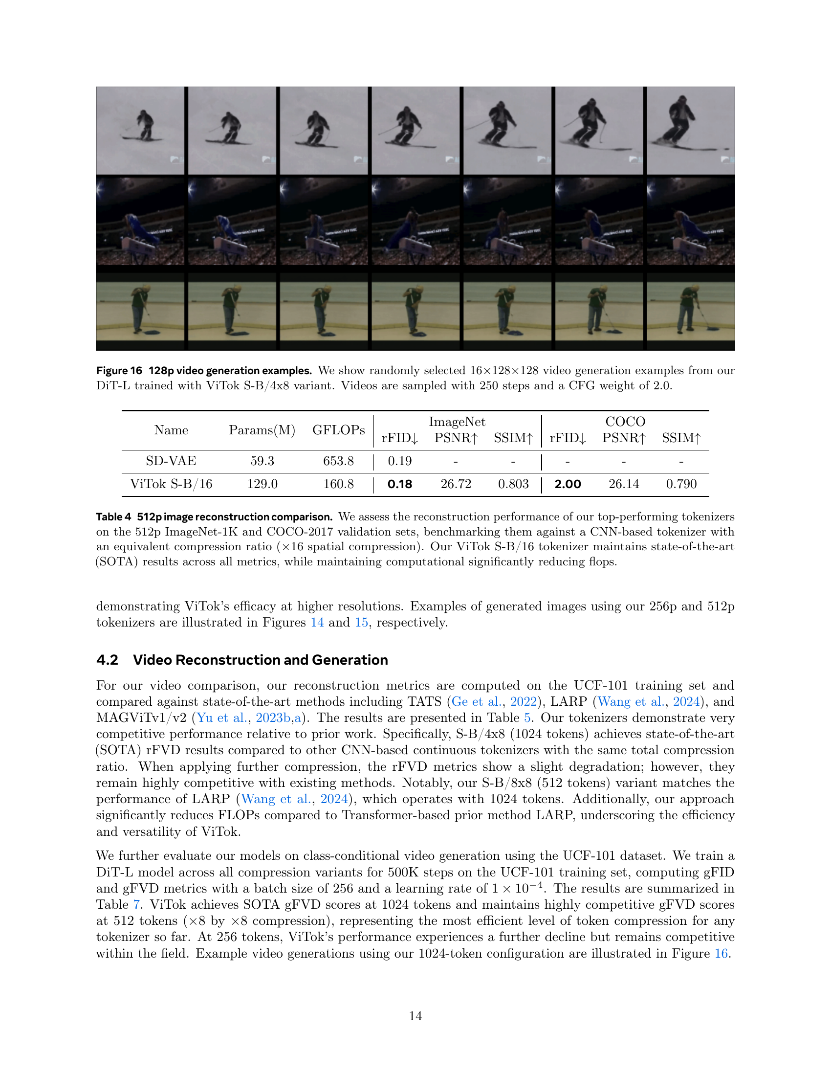
TL;DR#
Visual tokenization, encoding pixels into a latent space, is fundamental to image and video generation. While recent advances focus on generator scaling, the impact of scaling the tokenizer (auto-encoder) remains unclear, leading to suboptimal model performance. Prior methods rely on convolutional neural networks (CNNs) for tokenizers, limiting scalability and performance. The limited data also constrained effective tokenizer scaling.
This paper introduces ViTok, a novel Vision Transformer-based tokenizer, that addresses these issues. By using a Vision Transformer architecture and training on large-scale datasets, ViTok significantly improves reconstruction and generation quality. The authors find that scaling the decoder is more effective than scaling the encoder, which challenges conventional approaches. ViTok achieves state-of-the-art results in both image and video generation, outperforming existing methods with fewer computations.
Key Takeaways#
Why does it matter?#
This paper is crucial because it challenges the conventional wisdom in visual tokenization, which usually focuses on scaling generators while neglecting the tokenizer. By demonstrating the importance of scaling the auto-encoder, particularly the decoder, the study opens new avenues for improving both reconstruction and generation performance in image and video models. This is relevant to ongoing research in Transformer-based architectures and generative AI, suggesting improvements for a wide range of applications.
Visual Insights#

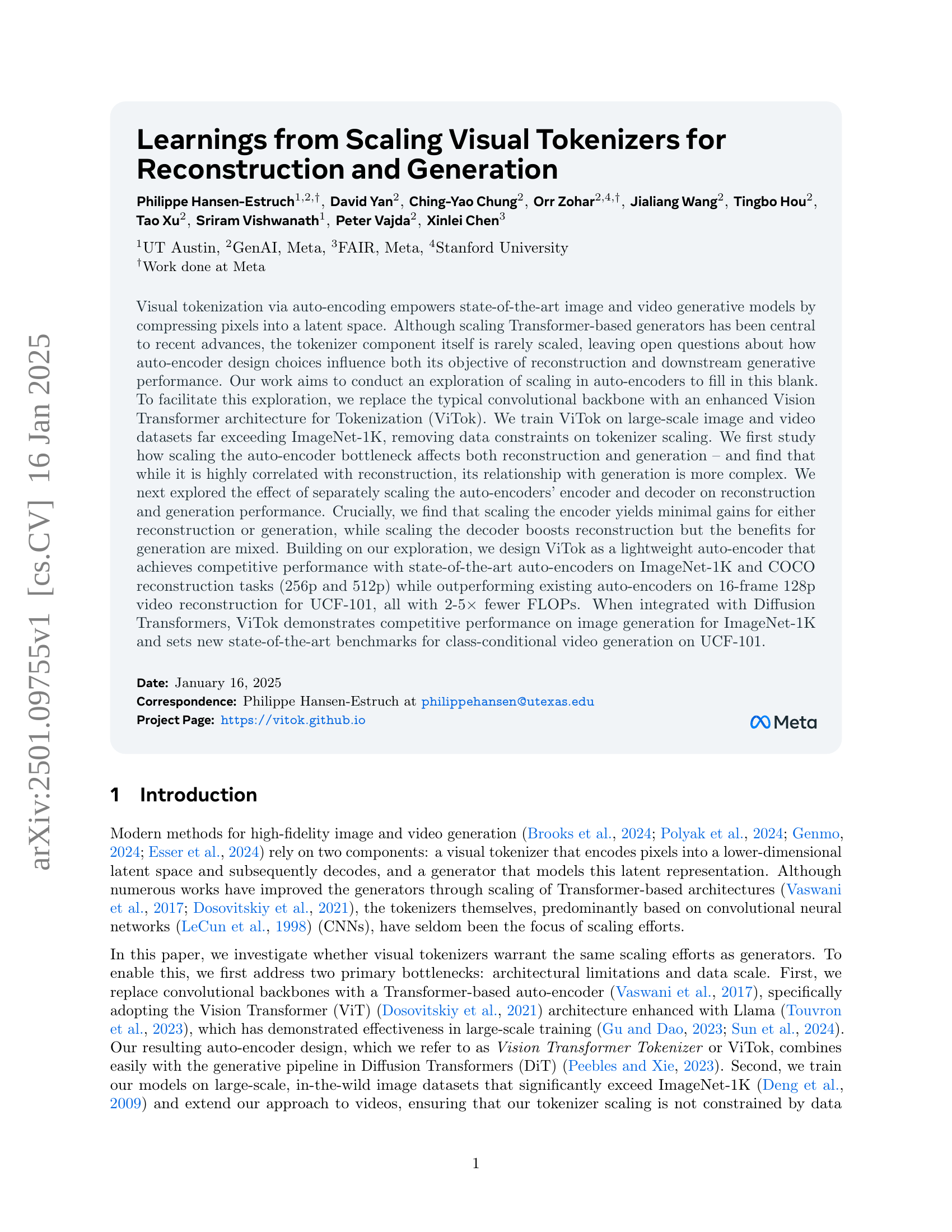
🔼 Figure 1 illustrates the key findings from scaling Vision Transformer Tokenizers (ViTok) for image and video reconstruction and generation. The left side shows the ViTok architecture, which replaces traditional CNN-based autoencoders with an asymmetric design integrating Vision Transformers (ViTs) and an enhanced Llama architecture. Visual inputs are embedded as patches or tubelets, encoded by a Llama Encoder, bottlenecked, upsampled by a larger Llama Decoder, and finally decoded to reconstruct the input. The right side summarizes the findings, highlighting the impact of scaling different components (encoder, decoder, bottleneck size) on reconstruction and generation performance. Color-coding helps visualize these effects. The figure also notes trade-offs in loss optimization strategies and the model’s adaptability for video. The best ViTok variant offers competitive performance and lower computational costs compared to existing methods.
read the caption
Figure 1: Our learnings from scaling ViTok. We showcase our ViTok architecture (left) and key findings (right) from scaling auto-encoders for image and video reconstruction and generation. We enhance traditional CNN-based auto-encoders by integrating Vision Transformers (ViTs) with an upgraded Llama architecture into an asymmetric auto-encoder framework forming Vision Transformer Tokenizer or ViTok. Visual inputs are embedded as patches or tubelets, processed by a compact Llama Encoder, and bottlenecked to create a latent code. The encoded representation is then upsampled and handled by a larger Llama Decoder to reconstruct the input. Color-coded text boxes highlight the effects of scaling the encoder, adjusting the bottleneck size, and expanding the decoder. Additionally, we discuss trade-offs in loss optimization and the model’s adaptability to video data. Our best performing ViTok variant achieves competitive performance with prior state-of-the-art tokenizers while reducing computational burden.
| Model | Hidden Dimension | Blocks | Heads | Parameters (M) | GFLOPs |
| Small (S) | 768 | 6 | 12 | 43.3 | 11.6 |
| Base (B) | 768 | 12 | 12 | 85.8 | 23.1 |
| Large (L) | 1152 | 24 | 16 | 383.7 | 101.8 |
🔼 This table details the different model sizes and computational costs (in FLOPs and parameters) for various configurations of the ViTok model. ViTok model configurations are described by a three-part identifier: (encoder size)-(decoder size)/(tubelet size). The encoder and decoder sizes can be Small (S), Base (B), or Large (L), representing different model complexities, each with a specific hidden dimension, number of blocks, and number of attention heads. Tubelet size refers to the spatial and temporal downsampling factors (q and p) during the embedding process. The table shows that while increasing the model size (e.g., from S to L) significantly increases both FLOPs and the number of parameters, adjustments have been made to the small model to enhance its performance.
read the caption
Table 1: Model Sizes and FLOPs for ViTok. We describe ViTok variants by specifying the encoder and decoder sizes separately, along with the tubelet sizes. For example, ViTok S-B/4x16 refers to a model with an encoder of size Small (S) and a decoder of size Base (B), using tubelet size q=4𝑞4q=4italic_q = 4 and p=16𝑝16p=16italic_p = 16. We modified the traditional Small (S) model by increasing its hidden dimension from 384 to 768 and reducing the number of blocks from 12 to 6 to increase flops and parameters slightly. Additionally, for the Large (L) model, we increased the hidden dimension to 1152 from 1024 to ensure divisibility by 3 for 3D RoPE integration.
In-depth insights#
ViTok Architecture#
The ViTok architecture is a novel approach to visual tokenization that significantly improves upon traditional methods by leveraging the power of Vision Transformers (ViTs). Instead of relying on convolutional neural networks (CNNs), ViTok employs an enhanced ViT architecture combined with an upgraded Llama architecture for both its encoder and decoder. This Transformer-based design offers several key advantages. It is inherently scalable, allowing for easy adjustment of the model’s capacity through changes in the number of layers and hidden dimensions. ViTok addresses architectural limitations and data constraints often encountered with CNN-based tokenizers by effectively handling large-scale image and video datasets. Another critical aspect is the introduction of an asymmetric auto-encoder framework, where the decoder is significantly larger than the encoder. This design choice is shown to be highly effective for reconstruction tasks, demonstrating a notable ability to recover high-fidelity images and videos even with substantial compression. The paper’s key finding is the emphasis on the decoder’s role in balancing reconstruction quality and downstream generative performance. By carefully scaling the decoder, significant gains in reconstruction can be achieved, while the impact on generation is shown to be more complex, suggesting potential improvements in model design for future research.
Scaling Effects#
The research paper explores scaling effects in visual tokenizers, specifically focusing on how alterations to the autoencoder’s architecture and training impact both image reconstruction and generation. The core finding is that simply increasing the size of the model (scaling the encoder or decoder) does not guarantee improved performance. While scaling the bottleneck size enhances reconstruction, it can negatively affect generation. Scaling the decoder leads to better reconstruction but yields mixed results in generation, suggesting it functions partially as a generative model. Crucially, the study identifies the total number of floating-point operations (E) in the latent code as the primary bottleneck for reconstruction, irrespective of the encoder or decoder design or FLOPs used. These findings highlight the complex interplay between reconstruction and generation performance, emphasizing the need for a balanced approach to scaling visual tokenizers for optimal results in downstream generative tasks. Data limitations are also addressed by training on large-scale datasets, enabling a more thorough investigation into the effects of scaling.
E Bottleneck#
The research paper’s analysis of the ‘E Bottleneck’ reveals a crucial insight into the limitations of solely scaling autoencoders for enhanced visual generation. The total number of floating-point numbers (E) in the latent code acts as the primary bottleneck, strongly correlating with reconstruction quality metrics. Increasing E improves reconstruction but unexpectedly degrades generation performance beyond a certain point. This highlights that simply increasing the size of the autoencoder doesn’t guarantee better results, underscoring the complex interplay between reconstruction fidelity and generative capabilities. The findings suggest a careful balance is needed; a low E restricts reconstruction quality, whereas a high E, achieved by larger channel sizes, complicates the generative model’s convergence and performance. The optimal E varies depending on other factors such as patch size, further emphasizing that a holistic approach to scaling is crucial for optimal performance in visual tokenization.
Decoder Role#
The research reveals a nuanced decoder role beyond simple reconstruction. Initially viewed as a component for reconstructing encoded data, the decoder increasingly acts as a generative model, particularly when using GAN loss functions. This transition is marked by a trade-off: higher fidelity to the original image (measured by PSNR/SSIM) is sacrificed for improved image quality (FID/IS). The results emphasize the decoder’s capacity to generate content, filling in details based on limited information. Scaling the decoder improves reconstruction but yields mixed results for generation, highlighting a complex interaction between reconstruction fidelity and generative capabilities. The authors’ exploration shows that optimizing for both aspects is crucial, implying that auto-encoder design should carefully balance these competing goals to maximize overall performance.
Future Work#
Future research directions stemming from this visual tokenizer scaling work could explore several promising avenues. Extending ViTok’s architecture to handle even higher-resolution images and videos is crucial, necessitating investigation into efficient memory management and computational strategies. A deeper exploration of the interplay between different loss functions and their impact on both reconstruction and generation quality warrants further study. This includes investigating novel loss formulations or weighting schemes that could better balance fidelity and perceptual quality. Incorporating more advanced techniques, like attention mechanisms or improved positional encodings, within the ViT architecture, may unlock further improvements in performance and efficiency. The effectiveness of ViTok with diverse generative models beyond diffusion transformers also needs examination. Finally, thorough analysis of the model’s robustness and generalization capabilities across various datasets and task domains is needed to ascertain its true practical value. Thorough ablation studies on various model components could provide a fine-grained understanding of the model’s strengths and weaknesses.
More visual insights#
More on figures

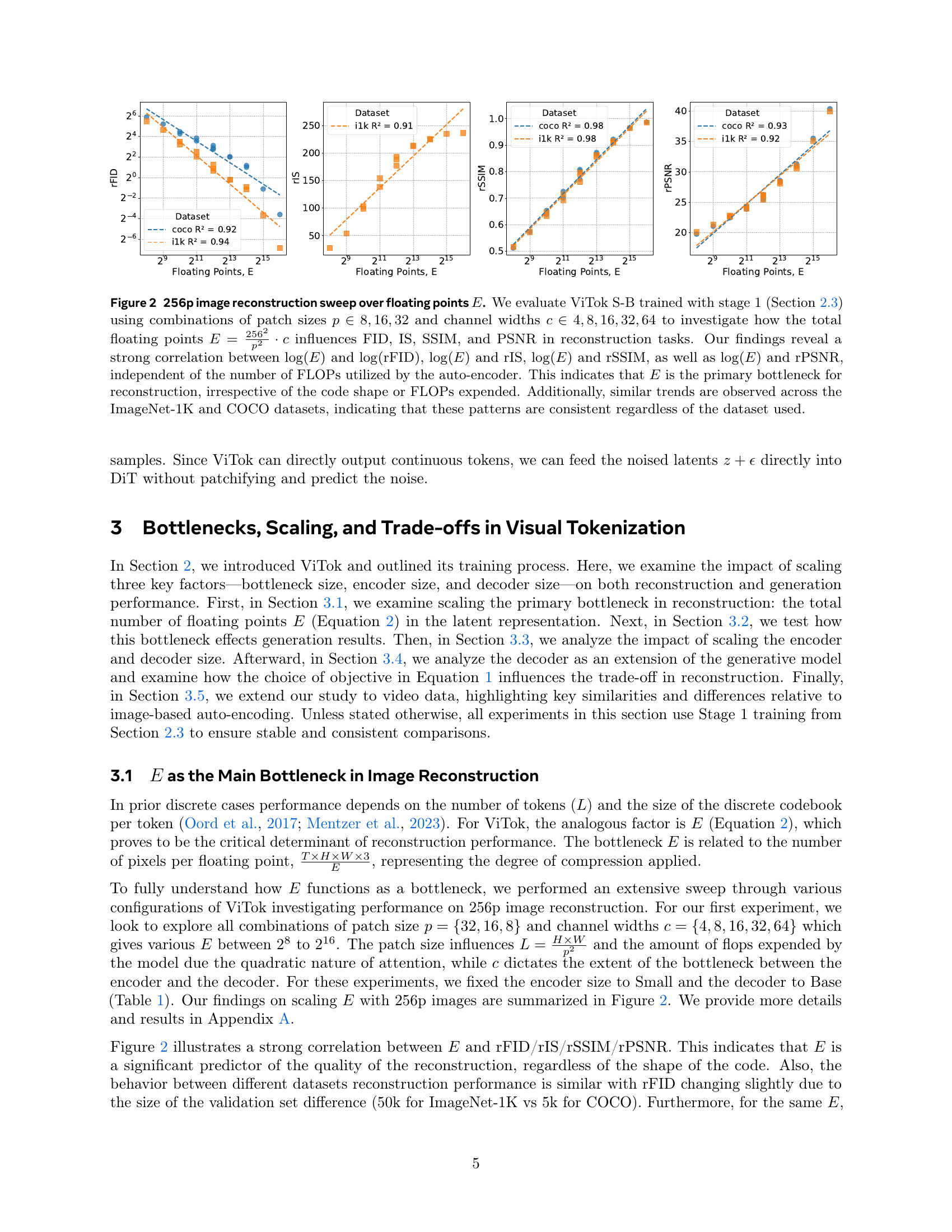
🔼 This figure shows the results of an experiment investigating the impact of the total number of floating-point numbers (E) in the latent representation on image reconstruction performance. The experiment varied the patch size (p) and the number of channels (c) in the ViTok model, while keeping the encoder size small and the decoder size base. The results show a strong positive correlation between the logarithm of E and the logarithm of reconstruction metrics (FID, IS, SSIM, PSNR), regardless of the computational cost (FLOPs). This suggests that E is the primary limiting factor for reconstruction quality, not the specific architecture or computational complexity. The consistent trends across ImageNet-1K and COCO datasets further support this conclusion.
read the caption
Figure 2: 256p image reconstruction sweep over floating points E𝐸Eitalic_E. We evaluate ViTok S-B trained with stage 1 (Section 2.3) using combinations of patch sizes p∈8,16,32𝑝81632p\in{8,16,32}italic_p ∈ 8 , 16 , 32 and channel widths c∈4,8,16,32,64𝑐48163264c\in{4,8,16,32,64}italic_c ∈ 4 , 8 , 16 , 32 , 64 to investigate how the total floating points E=2562p2⋅c𝐸⋅superscript2562superscript𝑝2𝑐E=\frac{256^{2}}{p^{2}}\cdot citalic_E = divide start_ARG 256 start_POSTSUPERSCRIPT 2 end_POSTSUPERSCRIPT end_ARG start_ARG italic_p start_POSTSUPERSCRIPT 2 end_POSTSUPERSCRIPT end_ARG ⋅ italic_c influences FID, IS, SSIM, and PSNR in reconstruction tasks. Our findings reveal a strong correlation between log(E)𝐸\log(E)roman_log ( italic_E ) and log(rFID)rFID\log(\text{rFID})roman_log ( rFID ), log(E)𝐸\log(E)roman_log ( italic_E ) and rIS, log(E)𝐸\log(E)roman_log ( italic_E ) and rSSIM, as well as log(E)𝐸\log(E)roman_log ( italic_E ) and rPSNR, independent of the number of FLOPs utilized by the auto-encoder. This indicates that E𝐸Eitalic_E is the primary bottleneck for reconstruction, irrespective of the code shape or FLOPs expended. Additionally, similar trends are observed across the ImageNet-1K and COCO datasets, indicating that these patterns are consistent regardless of the dataset used.

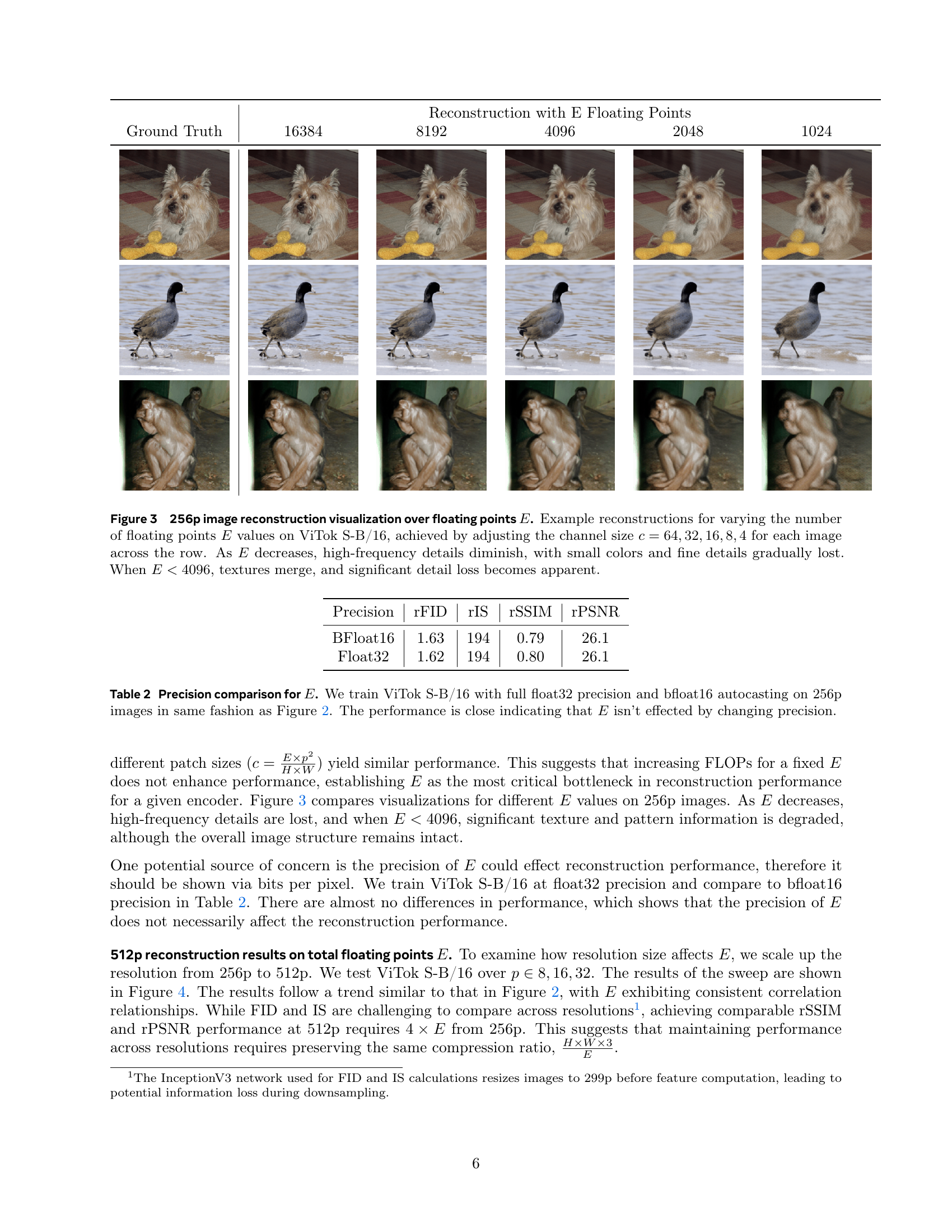
🔼 Figure 3 visualizes the effect of varying the total number of floating points (E) in the latent code on the quality of 256x256 pixel image reconstruction using the ViTok S-B/16 model. Each row represents a different value of E, achieved by adjusting the number of channels (c) in the latent space while keeping the patch size constant. As E decreases (moving from left to right), the amount of detail preserved in the reconstructed images decreases. High-frequency details, such as fine textures and small color variations, are lost first. When E falls below 4096, significant loss of image texture and detail becomes noticeable.
read the caption
Figure 3: 256p image reconstruction visualization over floating points E𝐸Eitalic_E. Example reconstructions for varying the number of floating points E𝐸Eitalic_E values on ViTok S-B/16, achieved by adjusting the channel size c=64,32,16,8,4𝑐64321684c={64,32,16,8,4}italic_c = 64 , 32 , 16 , 8 , 4 for each image across the row. As E𝐸Eitalic_E decreases, high-frequency details diminish, with small colors and fine details gradually lost. When E<4096𝐸4096E<4096italic_E < 4096, textures merge, and significant detail loss becomes apparent.

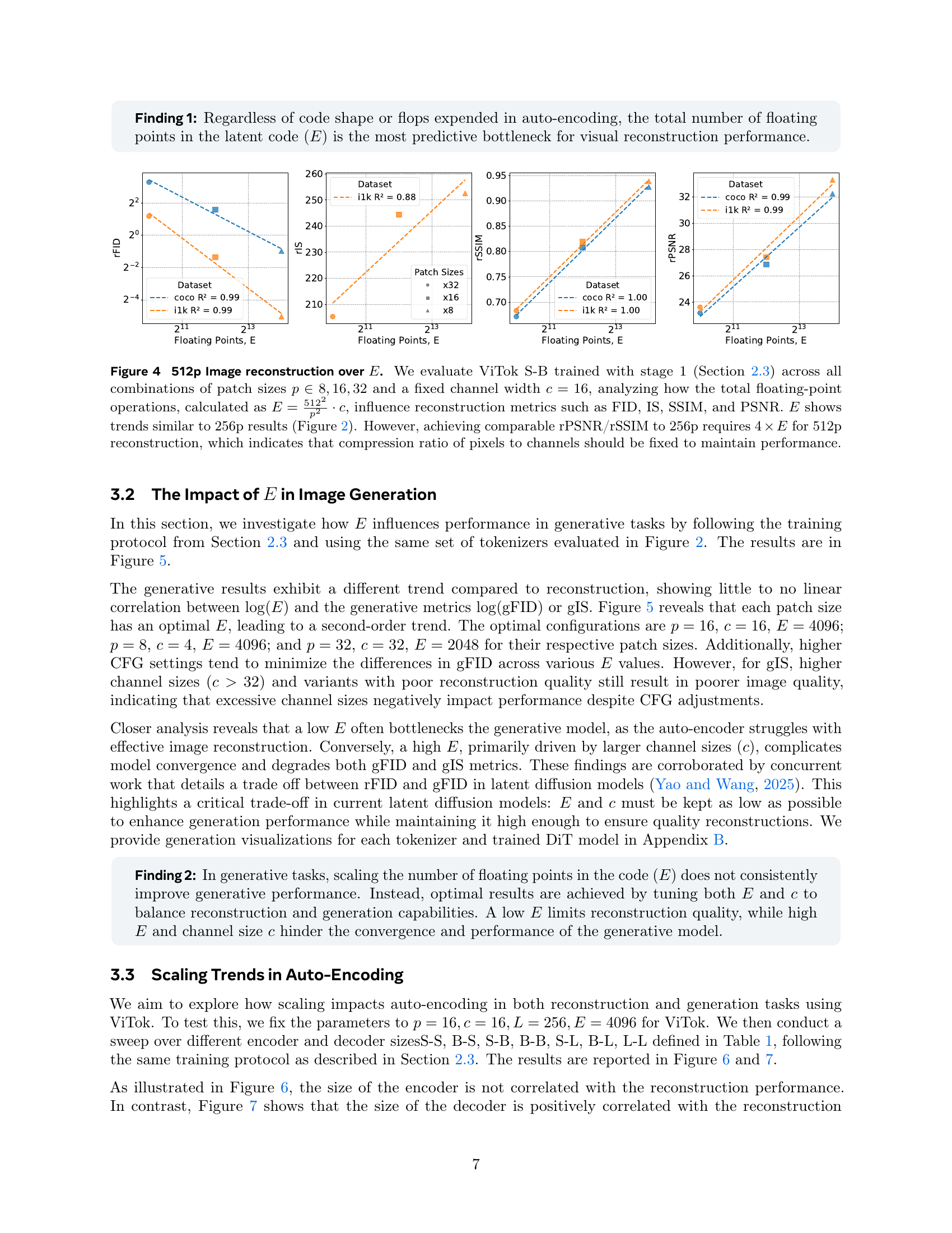
🔼 Figure 4 investigates the impact of the total number of floating-point operations (E) on the quality of 512p image reconstruction using the ViTok S-B model. The experiment systematically varies patch sizes (p) while keeping the channel width (c) constant at 16. The results show a strong correlation between E and reconstruction metrics (FID, IS, SSIM, PSNR), consistent with the findings from the 256p experiment in Figure 2. A key observation is that maintaining comparable reconstruction quality at 512p resolution requires four times the number of floating-point operations (4xE) compared to 256p, highlighting the importance of maintaining a consistent compression ratio (pixels to channels) for optimal reconstruction performance.
read the caption
Figure 4: 512p Image reconstruction over E𝐸Eitalic_E. We evaluate ViTok S-B trained with stage 1 (Section 2.3) across all combinations of patch sizes p∈8,16,32𝑝81632p\in{8,16,32}italic_p ∈ 8 , 16 , 32 and a fixed channel width c=16𝑐16c=16italic_c = 16, analyzing how the total floating-point operations, calculated as E=5122p2⋅c𝐸⋅superscript5122superscript𝑝2𝑐E=\frac{512^{2}}{p^{2}}\cdot citalic_E = divide start_ARG 512 start_POSTSUPERSCRIPT 2 end_POSTSUPERSCRIPT end_ARG start_ARG italic_p start_POSTSUPERSCRIPT 2 end_POSTSUPERSCRIPT end_ARG ⋅ italic_c, influence reconstruction metrics such as FID, IS, SSIM, and PSNR. E𝐸Eitalic_E shows trends similar to 256p results (Figure 2). However, achieving comparable rPSNR/rSSIM to 256p requires 4×E4𝐸4\times E4 × italic_E for 512p reconstruction, which indicates that compression ratio of pixels to channels should be fixed to maintain performance.

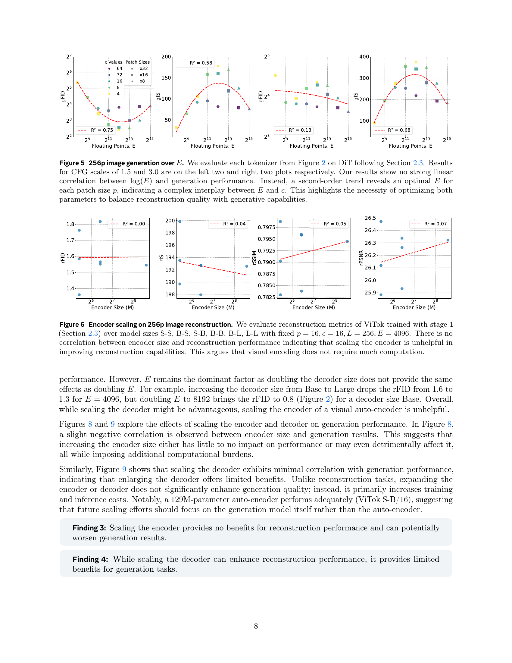
🔼 Figure 5 examines how the total number of floating points in the latent code (E), a key bottleneck in the model, impacts the quality of generated images. The figure presents four plots, each showing the relationship between E and two key metrics: gFID and gIS, which measure the quality of generated images and their diversity, respectively. Each plot corresponds to a different CFG (classifier-free guidance) scale (1.5 or 3.0), which affects the balance between image quality and adherence to the input prompt. The results show that for a given patch size (p), there’s an optimal E that yields the best performance. There’s no simple linear relationship, but rather a second-order curve indicating that either too small or too large an E hinders image generation quality.
read the caption
Figure 5: 256p image generation over E𝐸Eitalic_E. We evaluate each tokenizer from Figure 2 on DiT following Section 2.3. Results for CFG scales of 1.5 and 3.0 are on the left two and right two plots respectively. Our results show no strong linear correlation between log(E)𝐸\log(E)roman_log ( italic_E ) and generation performance. Instead, a second-order trend reveals an optimal E𝐸Eitalic_E for each patch size p𝑝pitalic_p, indicating a complex interplay between E𝐸Eitalic_E and c𝑐citalic_c. This highlights the necessity of optimizing both parameters to balance reconstruction quality with generative capabilities.

🔼 This figure analyzes the effect of scaling the encoder size on 256p image reconstruction quality using the ViTok model. The experiment controls for other variables by keeping the patch size (p), channel width (c), number of tokens (L), and total number of floating points (E) constant. The results show that there is no significant correlation between the size of the encoder and the reconstruction metrics. This suggests that increasing the complexity of the encoder does not necessarily lead to better reconstruction performance, indicating that visual encoding might not require extensive computational resources.
read the caption
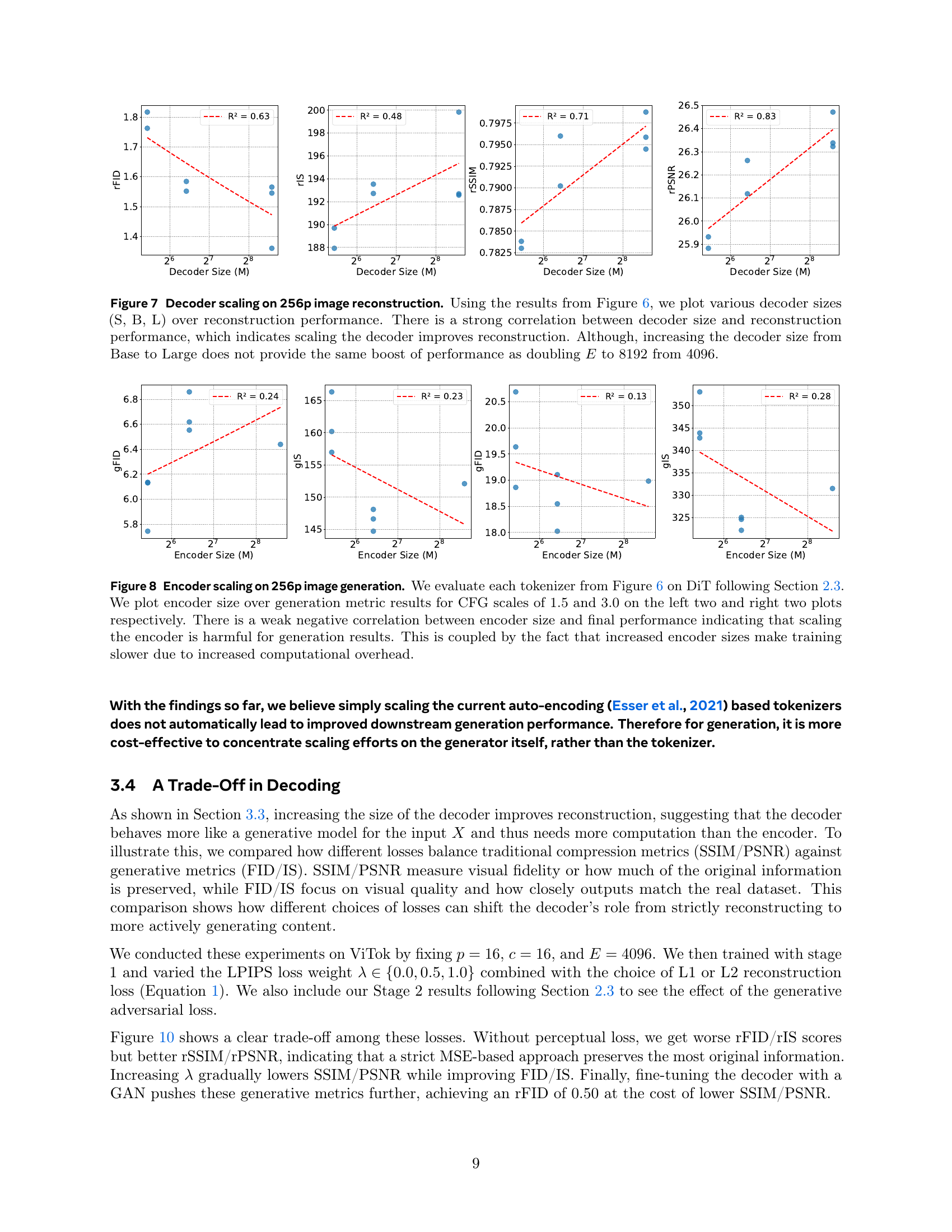
Figure 6: Encoder scaling on 256p image reconstruction. We evaluate reconstruction metrics of ViTok trained with stage 1 (Section 2.3) over model sizes S-S, B-S, S-B, B-B, B-L, L-L with fixed p=16,c=16,L=256,E=4096formulae-sequence𝑝16formulae-sequence𝑐16formulae-sequence𝐿256𝐸4096p=16,c=16,L=256,E=4096italic_p = 16 , italic_c = 16 , italic_L = 256 , italic_E = 4096. There is no correlation between encoder size and reconstruction performance indicating that scaling the encoder is unhelpful in improving reconstruction capabilities. This argues that visual encoding does not require much computation.

🔼 Figure 7 investigates the impact of scaling the decoder size on the performance of the ViTok model in 256p image reconstruction. The figure shows a strong positive correlation between decoder size and reconstruction quality, as measured by metrics like FID, suggesting that larger decoders generally lead to better reconstruction. However, the improvement plateaus when scaling the decoder from the ‘Base’ size to the ‘Large’ size; simply increasing the decoder size does not yield the same dramatic improvements observed when the total number of floating points in the latent code (E) is doubled.
read the caption
Figure 7: Decoder scaling on 256p image reconstruction. Using the results from Figure 6, we plot various decoder sizes (S, B, L) over reconstruction performance. There is a strong correlation between decoder size and reconstruction performance, which indicates scaling the decoder improves reconstruction. Although, increasing the decoder size from Base to Large does not provide the same boost of performance as doubling E𝐸Eitalic_E to 8192819281928192 from 4096409640964096.

🔼 Figure 8 explores the impact of scaling the encoder size of the ViTok architecture on the performance of image generation. The experiment uses the DiT model, following the training protocol described in Section 2.3 of the paper. Different encoder sizes (Small, Base, Large) are tested, and their performance is evaluated using two different CFG scales (1.5 and 3.0). The plots showcase the generation metrics (gFID) for each encoder size and CFG scale, revealing a weak negative correlation between encoder size and generation quality. Larger encoders do not improve, and may even slightly hinder, generation performance while increasing training time and computational cost.
read the caption
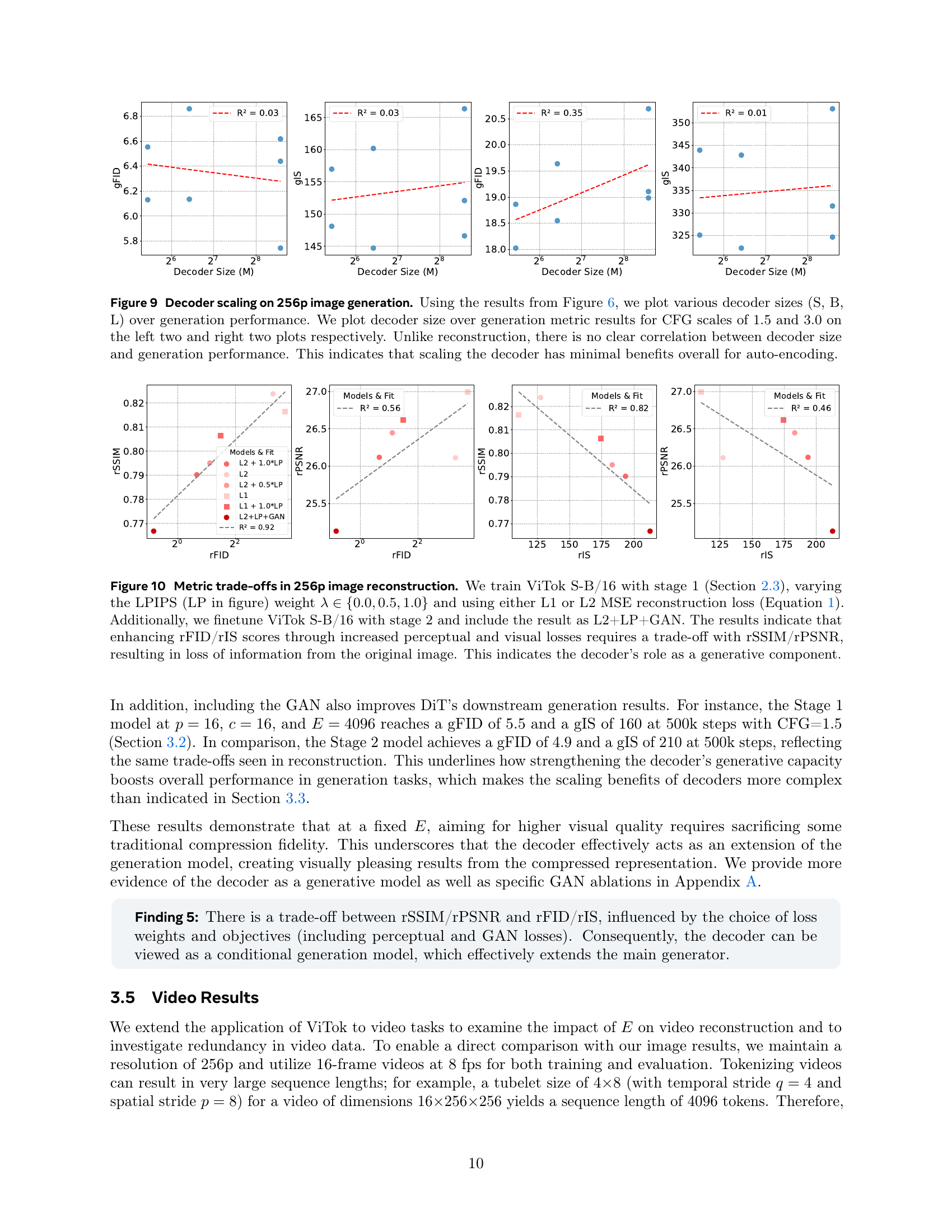
Figure 8: Encoder scaling on 256p image generation. We evaluate each tokenizer from Figure 6 on DiT following Section 2.3. We plot encoder size over generation metric results for CFG scales of 1.5 and 3.0 on the left two and right two plots respectively. There is a weak negative correlation between encoder size and final performance indicating that scaling the encoder is harmful for generation results. This is coupled by the fact that increased encoder sizes make training slower due to increased computational overhead.

🔼 Figure 9 explores the impact of scaling the decoder size on 256p image generation performance. It builds upon the results presented in Figure 6, which examined the effects of encoder scaling. The figure shows generation results (gFID and gIS) for different decoder sizes (Small, Base, Large), each tested with two different classifier-free guidance (CFG) scales (1.5 and 3.0). Unlike the findings for reconstruction tasks (where larger decoders improved performance), this figure demonstrates that decoder scaling has only minimal impact on image generation quality.
read the caption
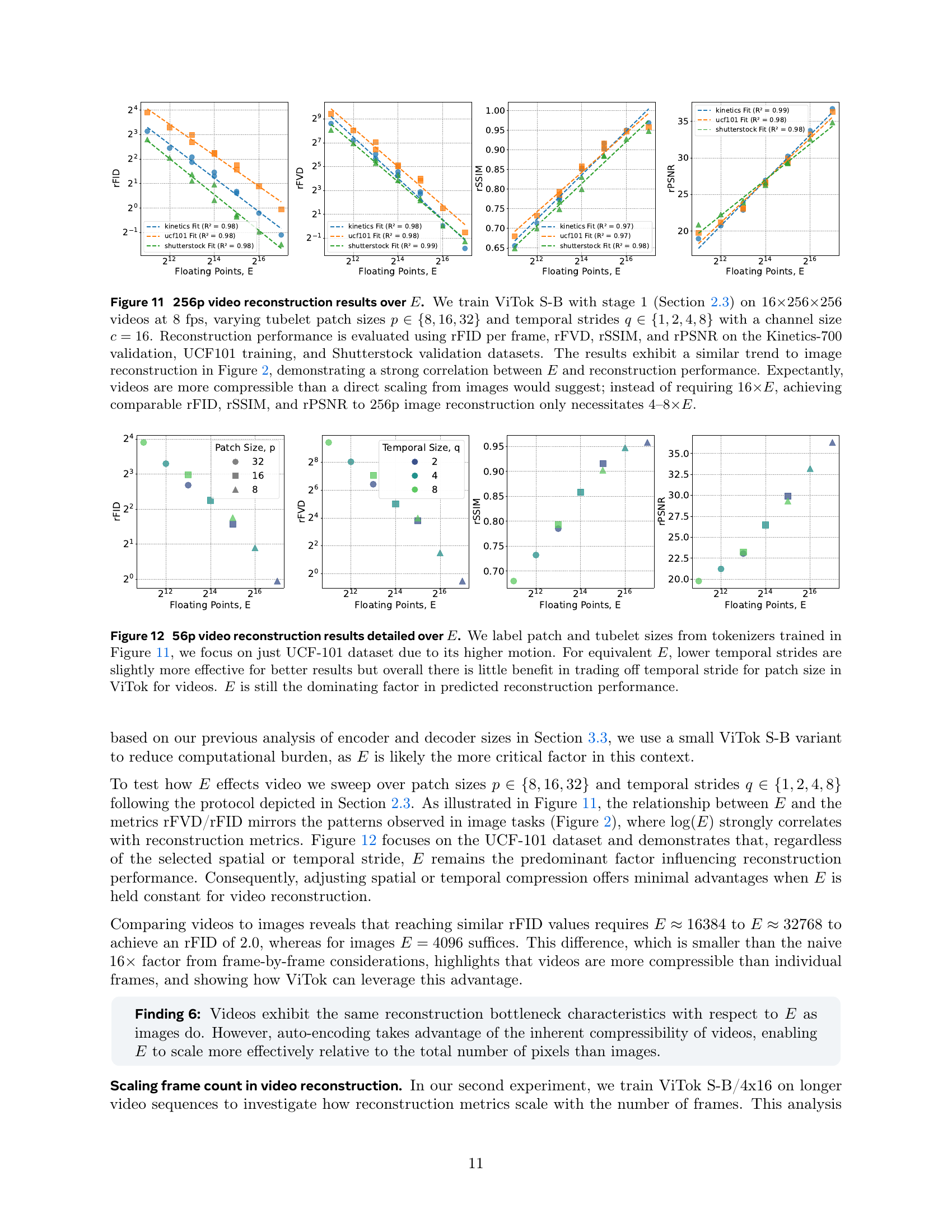
Figure 9: Decoder scaling on 256p image generation. Using the results from Figure 6, we plot various decoder sizes (S, B, L) over generation performance. We plot decoder size over generation metric results for CFG scales of 1.5 and 3.0 on the left two and right two plots respectively. Unlike reconstruction, there is no clear correlation between decoder size and generation performance. This indicates that scaling the decoder has minimal benefits overall for auto-encoding.
More on tables
| Reconstruction with E Floating Points | |||||
| Ground Truth | 16384 | 8192 | 4096 | 2048 | 1024 |
 |  |  |  |  |  |
 |  |  |  |  |  |
 |  |  |  |  |  |
🔼 This table compares the performance of the ViTok S-B/16 model trained with full float32 precision and bfloat16 autocasting on 256p images. The goal is to determine whether the precision of floating-point calculations in the model affects the reconstruction quality as measured by various metrics. The results demonstrate that the difference in reconstruction metrics between the two precision types is negligible, indicating that the model’s performance is not significantly impacted by using bfloat16 instead of float32.
read the caption
Table 2: Precision comparison for E𝐸Eitalic_E. We train ViTok S-B/16 with full float32 precision and bfloat16 autocasting on 256p images in same fashion as Figure 2. The performance is close indicating that E𝐸Eitalic_E isn’t effected by changing precision.
| Precision | rFID | rIS | rSSIM | rPSNR |
| BFloat16 | 1.63 | 194 | 0.79 | 26.1 |
| Float32 | 1.62 | 194 | 0.80 | 26.1 |
🔼 This table compares the performance of ViTok S-B/16 against other CNN-based continuous tokenizers on 256p ImageNet-1K and COCO-2017 validation sets. The comparison focuses on reconstruction quality, measured by rFID, PSNR, and SSIM, while also considering the computational efficiency (GFLOPS). ViTok S-B/16 achieves state-of-the-art (SOTA) rFID scores, outperforming others with significantly fewer FLOPs and maintaining competitive PSNR and SSIM. The table also shows that increasing the decoder size in ViTok improves reconstruction performance across all metrics.
read the caption
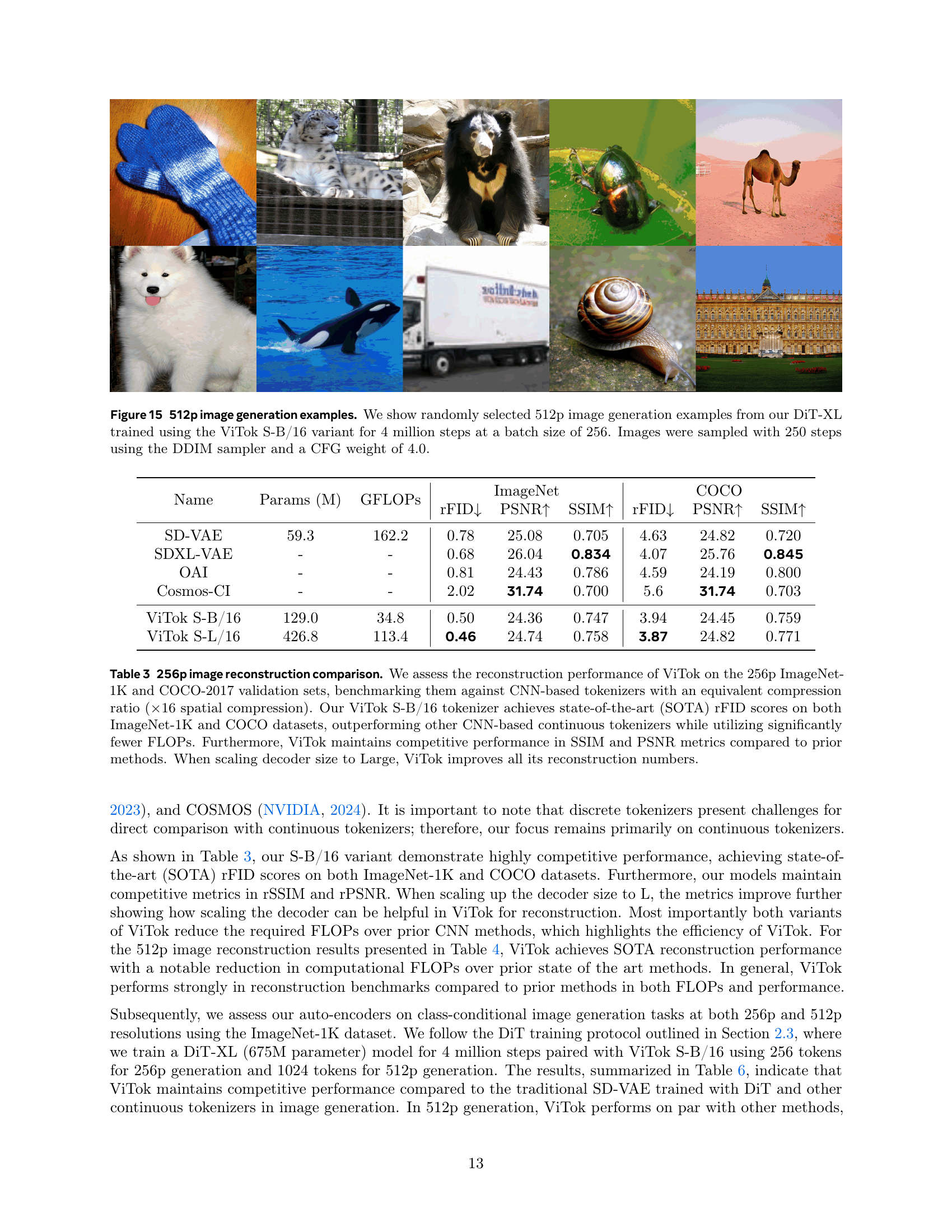
Table 3: 256p image reconstruction comparison. We assess the reconstruction performance of ViTok on the 256p ImageNet-1K and COCO-2017 validation sets, benchmarking them against CNN-based tokenizers with an equivalent compression ratio (×16absent16\times 16× 16 spatial compression). Our ViTok S-B/16 tokenizer achieves state-of-the-art (SOTA) rFID scores on both ImageNet-1K and COCO datasets, outperforming other CNN-based continuous tokenizers while utilizing significantly fewer FLOPs. Furthermore, ViTok maintains competitive performance in SSIM and PSNR metrics compared to prior methods. When scaling decoder size to Large, ViTok improves all its reconstruction numbers.
| Name | Params (M) | GFLOPs | ImageNet | COCO | ||||
| rFID | PSNR | SSIM | rFID | PSNR | SSIM | |||
| SD-VAE | 59.3 | 162.2 | 0.78 | 25.08 | 0.705 | 4.63 | 24.82 | 0.720 |
| SDXL-VAE | - | - | 0.68 | 26.04 | 0.834 | 4.07 | 25.76 | 0.845 |
| OAI | - | - | 0.81 | 24.43 | 0.786 | 4.59 | 24.19 | 0.800 |
| Cosmos-CI | - | - | 2.02 | 31.74 | 0.700 | 5.6 | 31.74 | 0.703 |
| ViTok S-B/16 | 129.0 | 34.8 | 0.50 | 24.36 | 0.747 | 3.94 | 24.45 | 0.759 |
| ViTok S-L/16 | 426.8 | 113.4 | 0.46 | 24.74 | 0.758 | 3.87 | 24.82 | 0.771 |
🔼 This table compares the performance of different visual tokenizers on 512x512 pixel image reconstruction tasks using the ImageNet-1K and COCO-2017 datasets. The comparison includes the number of parameters (in millions), the number of floating point operations (GFLOPs), and reconstruction metrics such as FID, PSNR, and SSIM. The key finding is that ViTok S-B/16 achieves state-of-the-art (SOTA) performance across all metrics, significantly reducing computational cost (GFLOPs) compared to alternative methods with similar compression ratios (16x spatial compression).
read the caption
Table 4: 512p image reconstruction comparison. We assess the reconstruction performance of our top-performing tokenizers on the 512p ImageNet-1K and COCO-2017 validation sets, benchmarking them against a CNN-based tokenizer with an equivalent compression ratio (×16absent16\times 16× 16 spatial compression). Our ViTok S-B/16 tokenizer maintains state-of-the-art (SOTA) results across all metrics, while maintaining computational significantly reducing flops.
| Name | Params(M) | GFLOPs | ImageNet | COCO | ||||
| rFID | PSNR | SSIM | rFID | PSNR | SSIM | |||
| SD-VAE | 59.3 | 653.8 | 0.19 | - | - | - | - | - |
| ViTok S-B/16 | 129.0 | 160.8 | 0.18 | 26.72 | 0.803 | 2.00 | 26.14 | 0.790 |
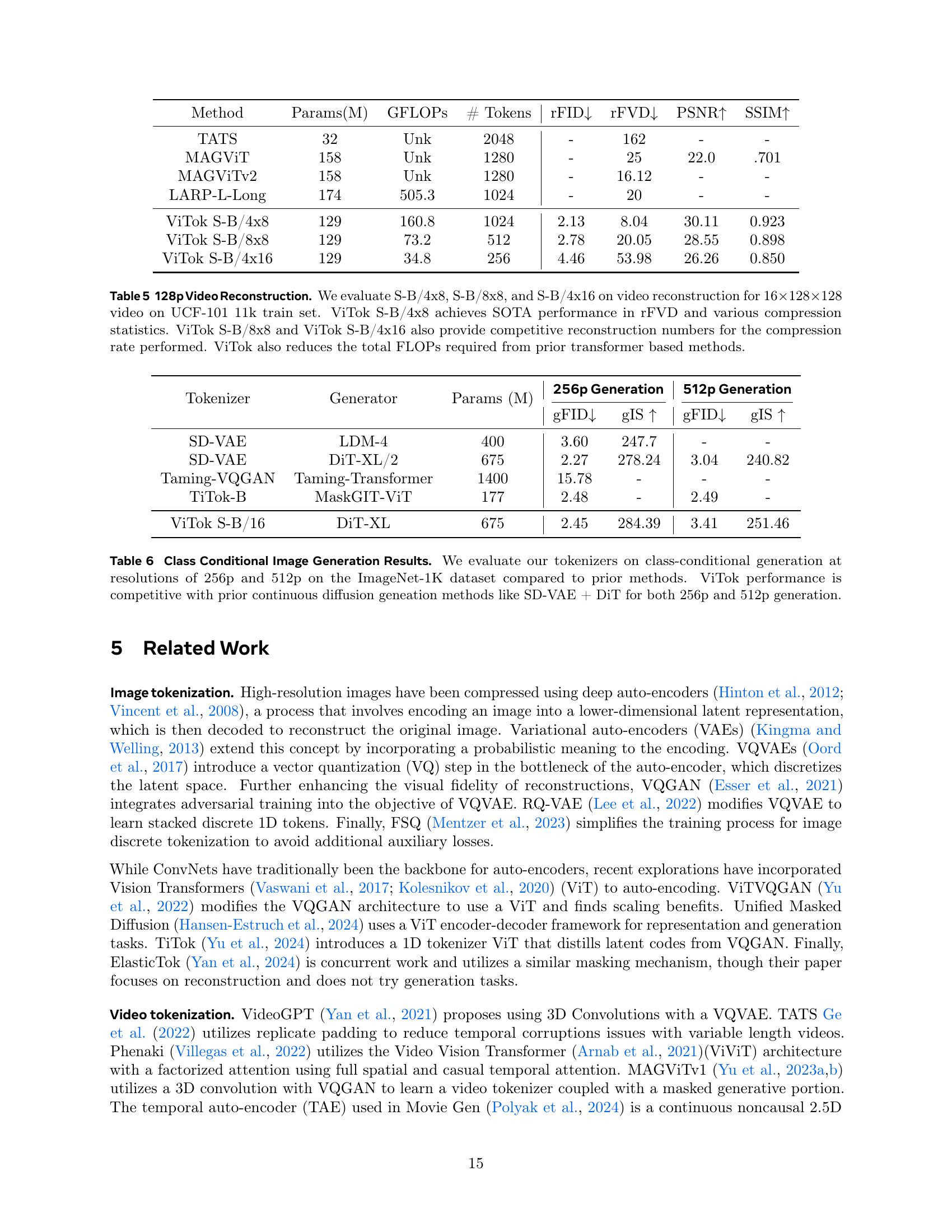
🔼 This table presents a comparison of video reconstruction performance using different ViTok configurations and other state-of-the-art methods on the UCF-101 dataset. The models are evaluated on 16-frame videos with a resolution of 128x128 pixels. Key metrics include rFVD (lower is better), PSNR (higher is better), and SSIM (higher is better). The table shows ViTok’s competitive performance and reduced computational cost (GFLOPs) compared to prior transformer-based methods. Different ViTok configurations vary in their encoder/decoder sizes and resulting compression ratios, illustrating a tradeoff between computational efficiency and reconstruction quality.
read the caption
Table 5: 128p Video Reconstruction. We evaluate S-B/4x8, S-B/8x8, and S-B/4x16 on video reconstruction for 16×\times×128×\times×128 video on UCF-101 11k train set. ViTok S-B/4x8 achieves SOTA performance in rFVD and various compression statistics. ViTok S-B/8x8 and ViTok S-B/4x16 also provide competitive reconstruction numbers for the compression rate performed. ViTok also reduces the total FLOPs required from prior transformer based methods.
| Method | Params(M) | GFLOPs | # Tokens | rFID | rFVD | PSNR | SSIM |
| TATS | 32 | Unk | 2048 | - | 162 | - | - |
| MAGViT | 158 | Unk | 1280 | - | 25 | 22.0 | .701 |
| MAGViTv2 | 158 | Unk | 1280 | - | 16.12 | - | - |
| LARP-L-Long | 174 | 505.3 | 1024 | - | 20 | - | - |
| ViTok S-B/4x8 | 129 | 160.8 | 1024 | 2.13 | 8.04 | 30.11 | 0.923 |
| ViTok S-B/8x8 | 129 | 73.2 | 512 | 2.78 | 20.05 | 28.55 | 0.898 |
| ViTok S-B/4x16 | 129 | 34.8 | 256 | 4.46 | 53.98 | 26.26 | 0.850 |
🔼 This table presents a comparison of class-conditional image generation results at 256x256 and 512x512 resolutions using the ImageNet-1K dataset. The performance of various tokenizers, including the proposed ViTok model and several state-of-the-art methods (SD-VAE + DiT), is evaluated based on the gFID and gIS scores. The table showcases the competitiveness of ViTok, which achieves comparable results to existing continuous diffusion generation methods.
read the caption
Table 6: Class Conditional Image Generation Results. We evaluate our tokenizers on class-conditional generation at resolutions of 256p and 512p on the ImageNet-1K dataset compared to prior methods. ViTok performance is competitive with prior continuous diffusion geneation methods like SD-VAE + DiT for both 256p and 512p generation.
| Tokenizer | Generator | Params (M) | 256p Generation | 512p Generation | ||
| gFID | gIS | gFID | gIS | |||
| SD-VAE | LDM-4 | 400 | 3.60 | 247.7 | - | - |
| SD-VAE | DiT-XL/2 | 675 | 2.27 | 278.24 | 3.04 | 240.82 |
| Taming-VQGAN | Taming-Transformer | 1400 | 15.78 | - | - | - |
| TiTok-B | MaskGIT-ViT | 177 | 2.48 | - | 2.49 | - |
| ViTok S-B/16 | DiT-XL | 675 | 2.45 | 284.39 | 3.41 | 251.46 |
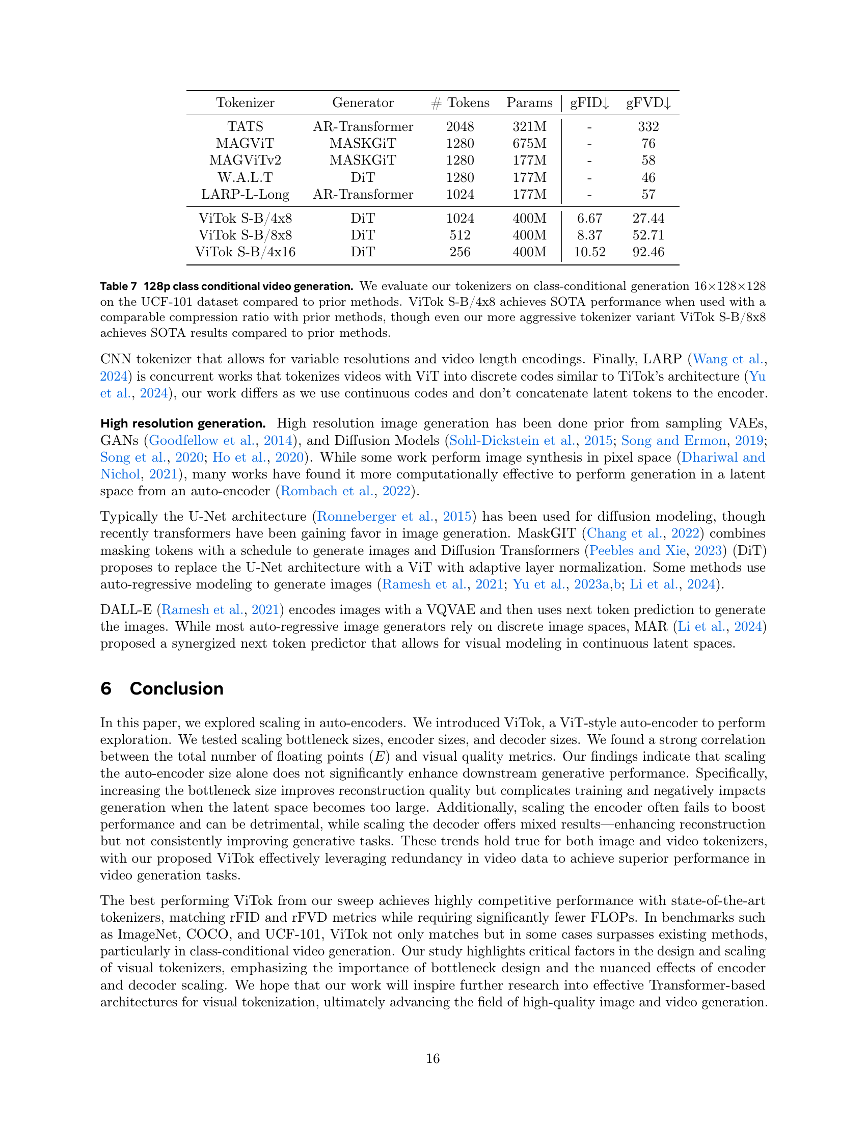
🔼 This table presents a comparison of various tokenizers’ performance on class-conditional video generation tasks. The evaluation focuses on 16-frame videos with a resolution of 128x128 pixels from the UCF-101 dataset. Key metrics include the Fréchet Inception Distance (gFID) and the Fréchet Video Distance (gFVD), which assess the quality and similarity of the generated videos to real videos. The table compares ViTok variants (S-B/4x8, S-B/8x8, S-B/4x16) against other state-of-the-art tokenizers, highlighting ViTok’s superior performance in terms of gFID and gFVD while using a comparable compression ratio. Even the more aggressive ViTok variant (S-B/8x8) achieves state-of-the-art results.
read the caption
Table 7: 128p class conditional video generation. We evaluate our tokenizers on class-conditional generation 16×\times×128×\times×128 on the UCF-101 dataset compared to prior methods. ViTok S-B/4x8 achieves SOTA performance when used with a comparable compression ratio with prior methods, though even our more aggressive tokenizer variant ViTok S-B/8x8 achieves SOTA results compared to prior methods.
Full paper#
