TL;DR#
Large language models (LLMs) are computationally expensive, particularly during inference. Existing methods for improving efficiency often focus on uniform compression of key and value components, neglecting the varying impacts of each component on the model. This paper introduces limitations of the existing LLMs.
The paper proposes SIGMA, a new LLM architecture employing
DiffQKV attention, which differentially optimizes query, key, and value components based on their impact on performance and efficiency. This approach achieves significant inference speed improvements and is demonstrated through rigorous theoretical analysis and experimental results on the newly introduced AIMICIUS benchmark. Results show SIGMA significantly outperforming existing models in the system domain, indicating its potential for real-world applications.
Key Takeaways#
Why does it matter?#
This paper is crucial for researchers working on large language models (LLMs) and system optimization. It introduces a novel attention mechanism that significantly improves inference efficiency, directly addressing a major bottleneck in LLM deployment. The proposed benchmark, AIMICIUS, provides a valuable tool for evaluating LLMs in the system domain, a field that is gaining importance as AI becomes more integral to various systems. The findings open new avenues for research in efficient LLM architecture and system-specific LLM development.
Visual Insights#

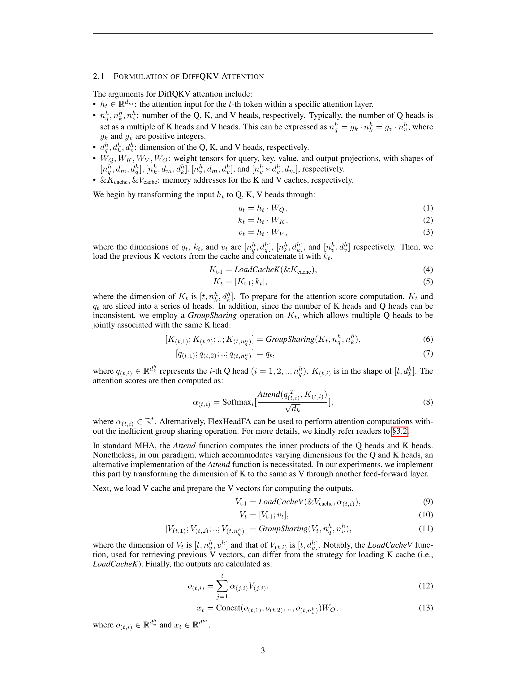
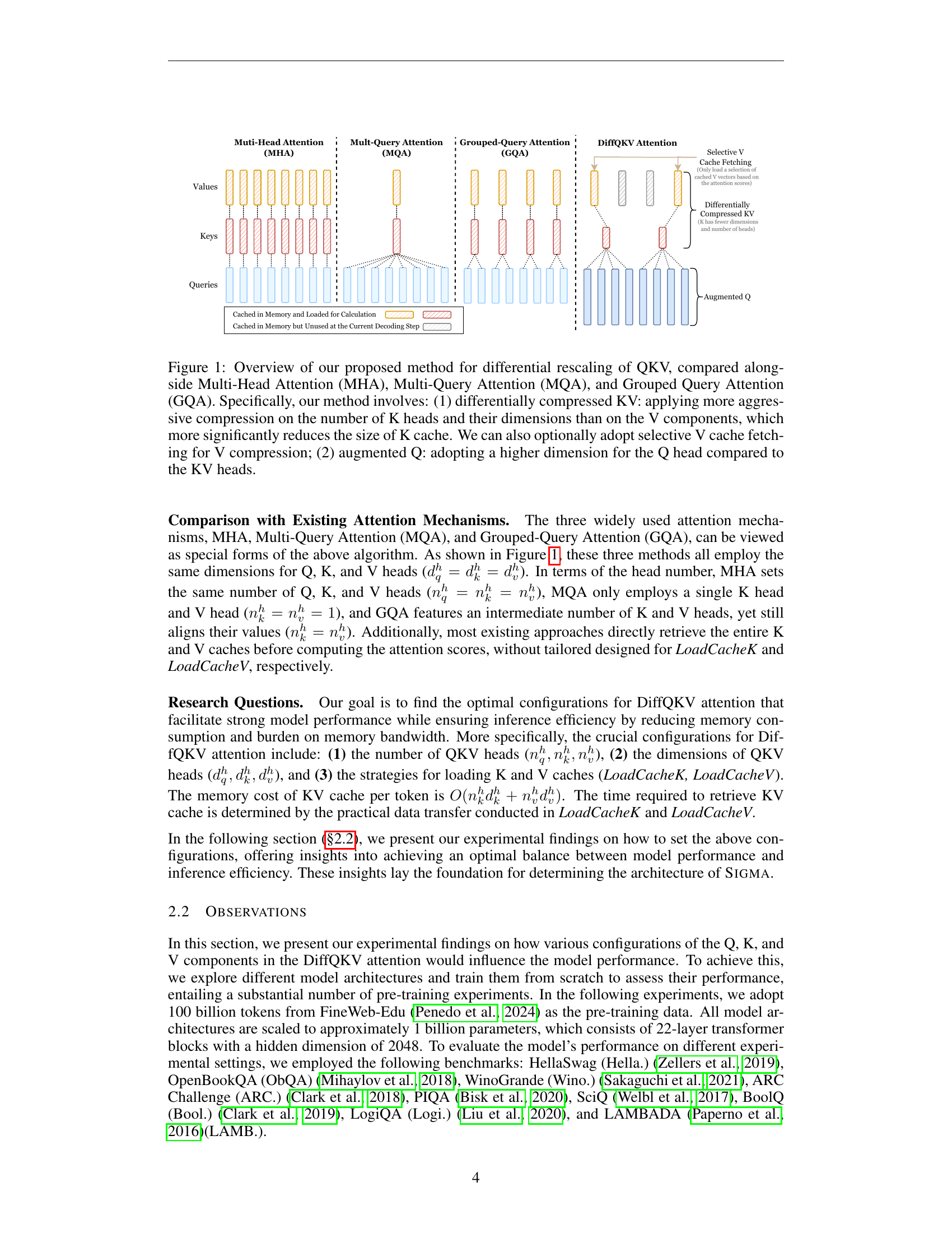
🔼 Figure 1 illustrates four different attention mechanisms: Multi-Head Attention (MHA), Multi-Query Attention (MQA), Grouped-Query Attention (GQA), and the proposed DiffQKV attention. The figure uses diagrams to highlight the key differences in how queries (Q), keys (K), and values (V) are handled in each method. Specifically, it shows that DiffQKV employs (1) differentially compressed KV: a more aggressive compression of K’s number of heads and dimensions compared to V to reduce K cache size, with optional selective V cache fetching for further compression, and (2) augmented Q: a higher dimension for Q heads than K or V heads to improve representation capability. The visual comparison allows readers to quickly grasp the architectural innovations introduced by DiffQKV and understand how it improves efficiency.
read the caption
Figure 1: Overview of our proposed method for differential rescaling of QKV, compared alongside Multi-Head Attention (MHA), Multi-Query Attention (MQA), and Grouped Query Attention (GQA). Specifically, our method involves: (1) differentially compressed KV: applying more aggressive compression on the number of K heads and their dimensions than on the V components, which more significantly reduces the size of K cache. We can also optionally adopt selective V cache fetching for V compression; (2) augmented Q: adopting a higher dimension for the Q head compared to the KV heads.
| Model | Overall | Commonsense & Comprehension | Continued | LM | ||||||
| Hella. | ObQA | Wino. | ARC. | PIQA | SciQ | Bool. | Logi. | LAMB. | ||
| MHA (==32) | 52.40 | 55.6 | 37.6 | 57.6 | 36.0 | 73.9 | 85.5 | 59.6 | 28.9 | 36.8 |
| -50% V Heads (=16) | 51.74 (0.66) | 55.5 | 39.6 | 55.0 | 35.9 | 71.6 | 85.9 | 56.9 | 28.3 | 37.0 |
| -50% K Heads (=16) | 52.83 (0.43) | 55.1 | 38.8 | 56.4 | 35.8 | 71.9 | 85.2 | 63.6 | 29.0 | 39.7 |
| GQA (==16) | 52.14 | 55.1 | 39.6 | 56.3 | 35.4 | 71.9 | 85.0 | 61.4 | 27.8 | 36.8 |
| -75% V Heads (=4) | 51.76 (0.38) | 54.0 | 38.2 | 55.6 | 34.8 | 72.7 | 85.0 | 60.3 | 29.9 | 35.3 |
| -75% K Heads (=4) | 51.97 (0.17) | 54.6 | 37.8 | 57.1 | 35.1 | 72.3 | 84.1 | 62.5 | 28.3 | 36.0 |
| GQA (==4) | 51.66 | 54.0 | 38.0 | 56.0 | 37.5 | 72.3 | 82.0 | 61.3 | 28.6 | 35.4 |
| -75% V Heads (=1) | 51.03 (0.63) | 53.5 | 38.4 | 57.0 | 35.1 | 72.1 | 82.6 | 56.9 | 28.4 | 35.1 |
| -75% K Heads (=1) | 51.67 (0.01) | 53.9 | 36.2 | 58.6 | 36.9 | 71.1 | 83.5 | 60.7 | 28.7 | 35.5 |
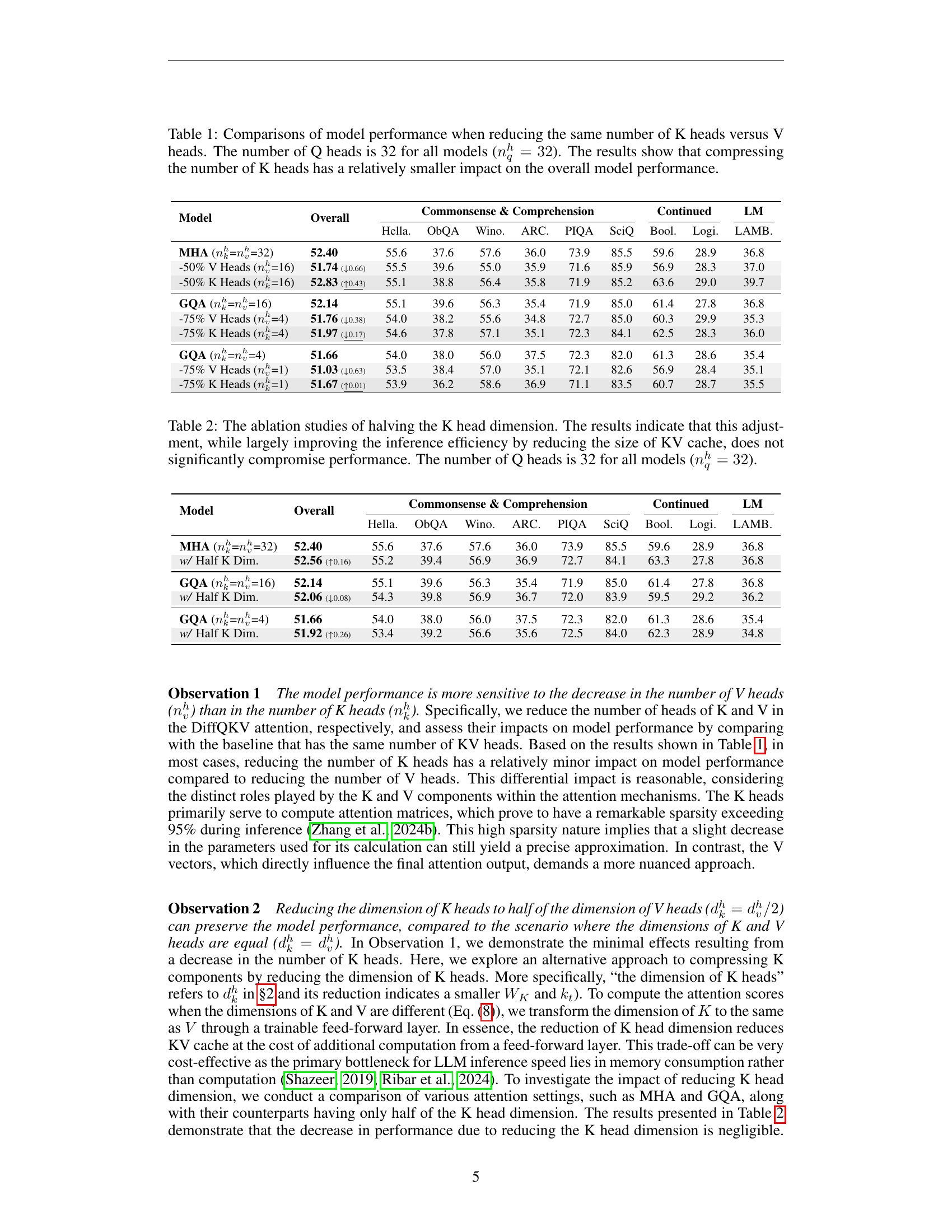
🔼 This table compares the performance of different models when reducing either the number of key heads (K) or value heads (V) by the same percentage. The number of query heads (Q) remains constant at 32 across all models. The results show that reducing the number of key heads has less of a negative impact on overall model performance compared to reducing the number of value heads. This is likely because key heads primarily serve to calculate attention matrices which tend to be quite sparse, whereas value heads directly impact the attention output.
read the caption
Table 1: Comparisons of model performance when reducing the same number of K heads versus V heads. The number of Q heads is 32 for all models (nqh=32superscriptsubscript𝑛𝑞ℎ32n_{q}^{h}=32italic_n start_POSTSUBSCRIPT italic_q end_POSTSUBSCRIPT start_POSTSUPERSCRIPT italic_h end_POSTSUPERSCRIPT = 32). The results show that compressing the number of K heads has a relatively smaller impact on the overall model performance.
In-depth insights#
DiffQKV Attention#
The proposed DiffQKV attention mechanism offers a novel approach to optimizing large language model (LLM) inference efficiency by differentially rescaling the Query (Q), Key (K), and Value (V) components within the attention mechanism. Unlike traditional methods that treat Q, K, and V uniformly, DiffQKV leverages the varying impact of each component on both performance and efficiency. This is achieved through two key techniques: differentially compressed KV, which compresses K more aggressively than V based on experimental observations of sensitivity, and augmented Q, which increases the dimensionality of the query component to compensate for the potential performance loss from KV compression. The result is a significant improvement in inference speed, particularly in long-context scenarios, while maintaining comparable performance to state-of-the-art models in general domains. Rigorous theoretical and empirical analyses support the effectiveness of DiffQKV, demonstrating that it outperforms conventional methods by mitigating KV cache bottlenecks and achieving a more efficient balance between model capacity and computational costs.
SIGMA Architecture#
The SIGMA architecture is designed for efficiency, particularly in handling long sequences. This is achieved through differential rescaling of Query, Key, and Value (QKV) components in the attention mechanism. The core innovation lies in its asymmetric treatment of K and V, recognizing their differing impact on both performance and efficiency. While aggressively compressing K, it uses less aggressive compression for V which is crucial as V directly affects final outputs. The augmented Q head compensates for any performance drop from KV compression, maintaining representation capacity without sacrificing inference speed. Further enhancements involve selective V cache fetching which loads only the most crucial vectors during inference, significantly lowering memory access and contributing to overall speed. These strategies work in concert to offer substantial inference speed improvements, especially in long-context scenarios, making it particularly suitable for system domain tasks which often involve lengthy sequences.
System Domain Focus#
A ‘System Domain Focus’ in a research paper would likely explore the application of AI models to optimize and manage AI systems themselves. This could involve using AI to monitor system performance, automatically diagnose and resolve issues, allocate resources efficiently, or even to design and improve future AI systems. The focus would likely delve into the unique challenges of this domain, such as the need for high reliability, security, and explainability in AI systems which manage critical infrastructure. Such a focus would also likely discuss the data requirements for training such models, which might include system logs, performance metrics, and configuration details. A key aspect would be benchmarking these AI systems for system management to establish their effectiveness against existing methods. The ultimate aim would be to demonstrate the potential for AI to not only improve AI model performance, but also to create a more sustainable and reliable development cycle for AI overall. This approach represents a meta-level application of AI, with significant implications for the future of AI technology.
Efficiency Analysis#
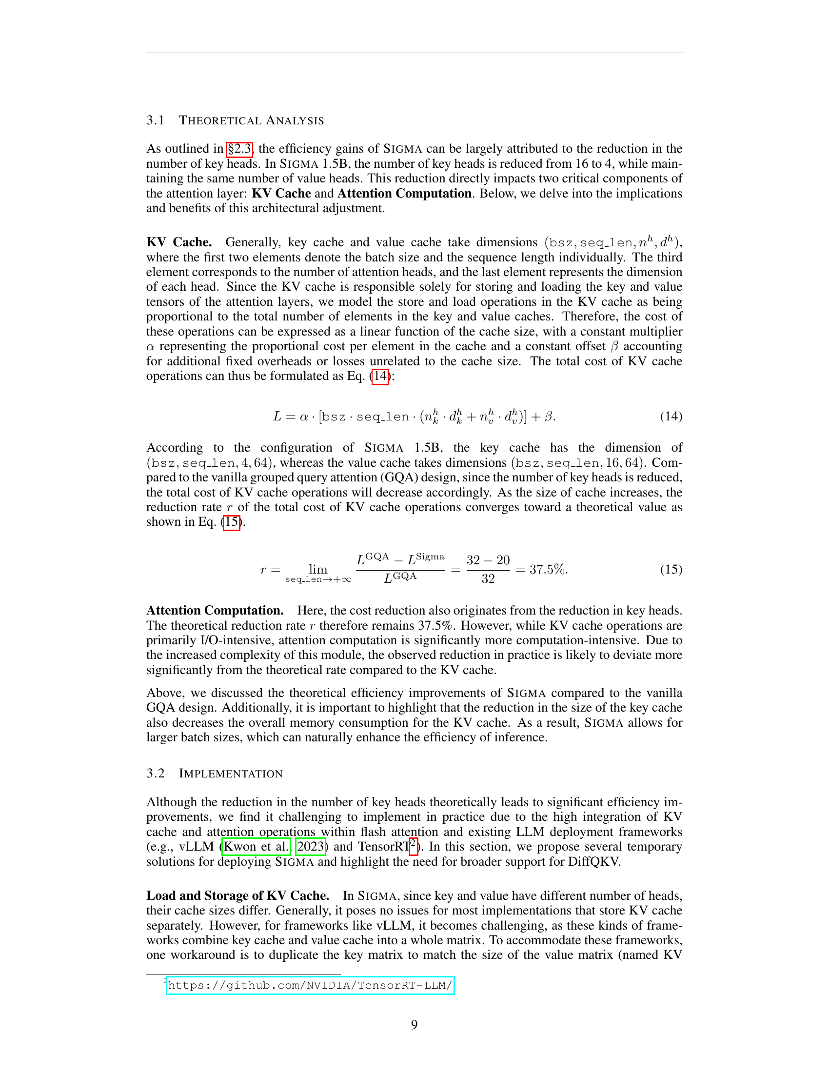
An efficiency analysis of a large language model (LLM) should thoroughly investigate the computational and memory aspects of its architecture. This involves examining the attention mechanism, specifically analyzing the impact of different designs (e.g., multi-head, grouped-query, and the proposed differential rescaling) on inference speed and memory usage. Theoretical analysis, using big O notation and mathematical models, can estimate the resource requirements of various operations. Empirical evaluations, using benchmarks on diverse tasks and hardware, are crucial to validate the theoretical analysis and demonstrate real-world performance gains. Such evaluation should include measuring key metrics like latency, throughput, and memory footprint, considering factors such as sequence length and batch size. The analysis must also discuss the trade-offs between efficiency and model performance, comparing the proposed method with existing state-of-the-art approaches. Finally, a discussion on implementation details and their impact on efficiency is also necessary. Optimizations, such as selective V-vector loading and efficient KV cache management, should be clearly explained and their effectiveness quantified.
Future Directions#
Future research directions for efficient large language models (LLMs) should prioritize reducing memory footprint and latency without sacrificing performance. This could involve exploring alternative attention mechanisms beyond DiffQKV, such as those utilizing sparse attention or more efficient matrix operations. Another avenue is optimizing the pre-training process itself by employing novel data augmentation techniques or focusing on carefully curated datasets that improve generalization and reduce overfitting. Expanding the AIMICIUS benchmark with a wider range of system domain tasks is crucial to comprehensively evaluate future LLMs, ensuring broader applicability and real-world relevance. Finally, investigating novel architectures that integrate techniques like model parallelism and quantization, while also exploring novel methods for efficient knowledge distillation from larger models, could lead to a new generation of resource-efficient and highly capable LLMs.
More visual insights#
More on figures

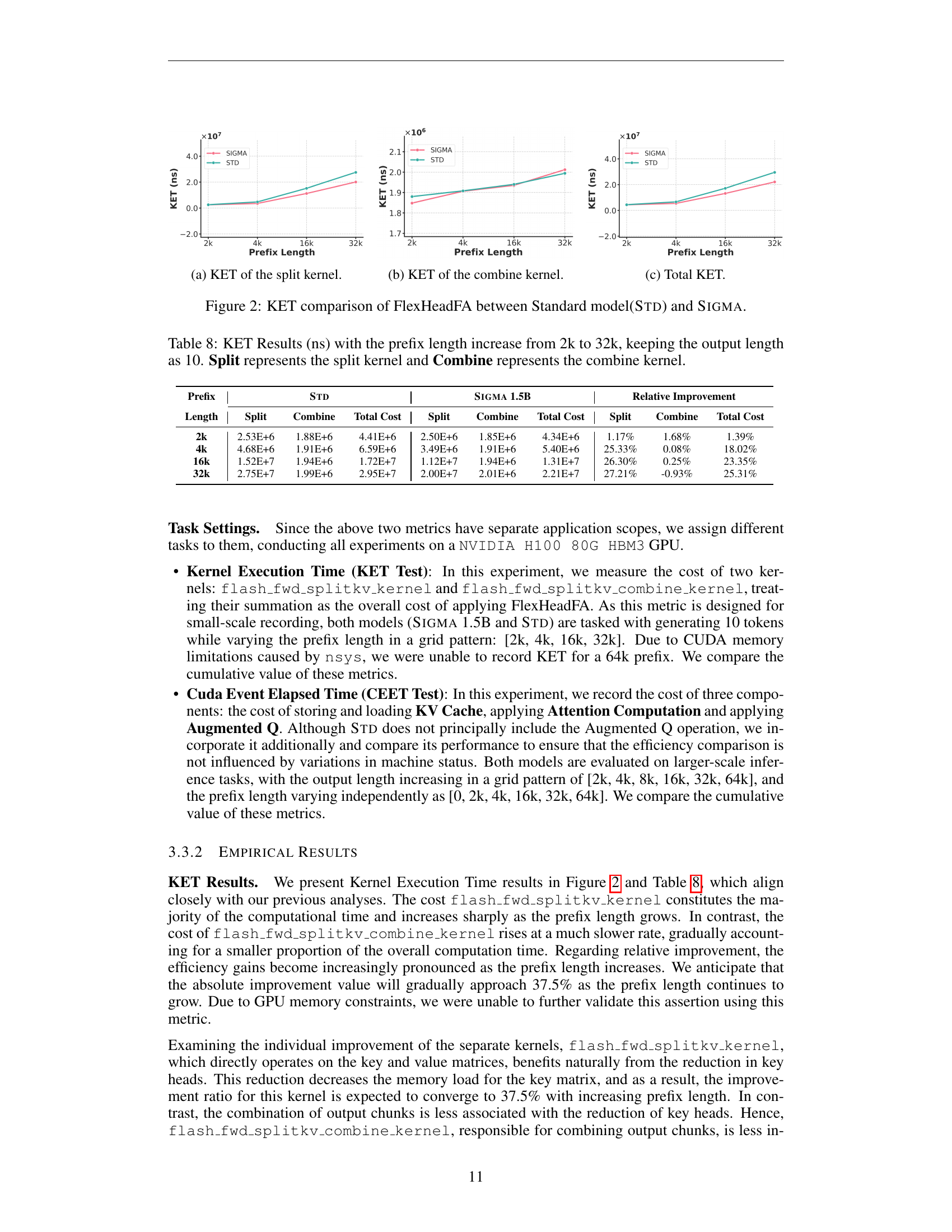
🔼 This figure shows the Kernel Execution Time (KET) for the split kernel of the FlexHeadFA attention mechanism. The KET is measured in nanoseconds (ns) and plotted against the prefix length, which represents the length of the input sequence. Two models, SIGMA and STD, are compared. The split kernel is one part of the Flash Attention 2 algorithm, responsible for dividing the key and value matrices into smaller chunks for efficient computation. This plot illustrates how the time taken by the split kernel changes as the input sequence length increases, revealing potential performance differences between the SIGMA and STD models in their attention mechanism.
read the caption
(a) KET of the split kernel.

🔼 This figure shows the Kernel Execution Time (KET) for the combine kernel in the FlexHeadFA attention mechanism. The combine kernel is responsible for assembling smaller output chunks into a complete output matrix during attention calculations. The graph likely plots KET (in nanoseconds) on the y-axis against prefix length (the length of the input sequence) on the x-axis. Separate lines probably represent the performance of the SIGMA model and the standard model (STD) for comparison. The purpose is to demonstrate the relative efficiency of SIGMA’s attention mechanism, especially as the input sequence grows longer, with a focus on the combine kernel’s contribution to the overall computation time.
read the caption
(b) KET of the combine kernel.

🔼 The figure shows the total kernel execution time (KET) for both the standard model (STD) and SIGMA 1.5B. The KET is the sum of the execution times for the ‘split’ and ‘combine’ kernels within the flash attention mechanism. The x-axis represents the prefix length, indicating the length of the input sequence processed before the current token. The y-axis represents the total kernel execution time in nanoseconds. The plot illustrates the impact of SIGMA’s DiffQKV attention mechanism on inference speed, particularly at longer prefix lengths, where SIGMA shows significantly improved performance compared to the standard model. The results are broken down to show the contribution of split and combine separately in order to demonstrate where the speed up comes from.
read the caption
(c) Total KET.

🔼 This figure compares the kernel execution time (KET) of the FlexHeadFA (Flexible Head Flash Attention) between the Standard model and the SIGMA model. The KET is broken down into the split and combine kernels. The x-axis represents the prefix length, and the y-axis shows the KET in nanoseconds. The figure shows how the efficiency of SIGMA improves, particularly as the prefix length increases. Different subplots focus on different components of the computation.
read the caption
Figure 2: KET comparison of FlexHeadFA between Standard model(Std) and Sigma.

🔼 The figure shows the CUDA Event Elapsed Time (CEET) results for different prefix lengths when the output length is fixed at 2k tokens. It compares the performance of SIGMA and the standard model (STD). The x-axis represents the prefix length, and the y-axis shows the CEET (in milliseconds). Different colored lines represent the CEET results for SIGMA (in blue) and STD (in red). The plot shows how the execution time of both models changes with the increasing prefix length.
read the caption
(a) Output Length =2kOutput Length 2𝑘\text{Output Length }=2kOutput Length = 2 italic_k.

🔼 This figure shows the Kernel Execution Time (KET) results for the combine kernel in the Flash Attention mechanism. The x-axis represents the prefix length of the input sequence, and the y-axis represents the execution time of the combine kernel. There are two lines in the graph, one for the standard model and one for the SIGMA model. The output length is fixed at 4k tokens. This figure demonstrates the efficiency gains of the SIGMA model over the standard model for the combine kernel operation when generating text with longer contexts, and shows that SIGMA’s gains become increasingly pronounced as the prefix length increases.
read the caption
(b) Output Length =4kabsent4𝑘=4k= 4 italic_k.

🔼 The figure shows the result of Kernel Execution Time (KET) test for the combine kernel in the flash attention mechanism. The x-axis represents the prefix length, and the y-axis represents the execution time of the combine kernel in nanoseconds. Two models are compared: the standard model (STD) and SIGMA. The output length is fixed at 8k tokens.
read the caption
(c) Output Length =8kabsent8𝑘=8k= 8 italic_k.

🔼 This figure displays the Cuda Event Elapsed Time (CEET) results for various components of the attention mechanism (KV Cache, Attention Computation, and Augmented Q) in the SIGMA and Standard models. The output length is fixed at 16k tokens, while the prefix length varies. The plot visually shows the time (in milliseconds) taken by each module for different prefix lengths, illustrating the performance difference between SIGMA (with DiffQKV attention) and the Standard model (with conventional grouped-query attention). The goal is to compare how the efficiency of these components changes in both models under different context lengths.
read the caption
(d) Output Length =16kabsent16𝑘=16k= 16 italic_k.

🔼 This figure displays the results from the Cuda Event Elapsed Time (CEET) test, specifically focusing on the scenario with an output length of 32,000 tokens. The CEET measures the end-to-end time of the attention computation. The figure likely shows how the total time for attention computation changes as the prefix length varies. This would help demonstrate SIGMA’s efficiency gain, particularly in longer sequences, where it surpasses other state-of-the-art models. The x-axis represents different prefix lengths, and the y-axis shows the corresponding CEET, allowing for a comparison between SIGMA and a standard model across various prefix lengths.
read the caption
(e) Output Length =32kabsent32𝑘=32k= 32 italic_k.

🔼 This figure displays the results of the Cuda Event Elapsed Time (CEET) test when the output length is 64k tokens. The CEET test measures the time taken to perform specific operations within the model, providing insights into efficiency and performance at varying prefix lengths. Different colored lines in the plot likely represent the performance of the model (SIGMA) compared to a baseline or standard model (STD) under different conditions. The x-axis represents the prefix length, and the y-axis displays the CEET in milliseconds.
read the caption
(f) Output Length =64kabsent64𝑘=64k= 64 italic_k.

🔼 The figure shows the absolute improvement in CUDA Event Elapsed Time (CEET) of SIGMA compared to the standard model (STD). The x-axis represents the prefix length, and the y-axis represents the absolute difference in milliseconds (ms) between the CEET of SIGMA and STD. Positive values indicate that SIGMA is faster than STD, while negative values indicate that SIGMA is slower.
read the caption
(g) Sigma’s absolute CEET improvment vs Std.

🔼 This figure shows the relative improvement in Cuda Event Elapsed Time (CEET) achieved by SIGMA compared to the standard model (STD). It displays the percentage difference in computation time between SIGMA and STD across various prefix lengths and output lengths. A positive value indicates that SIGMA is faster, while a negative value means STD is faster. The figure provides a visual representation of SIGMA’s efficiency gains in handling long sequences, showing how its performance advantage grows with increasing context size.
read the caption
(h) Sigma’s relative CEET improvment vs Std.

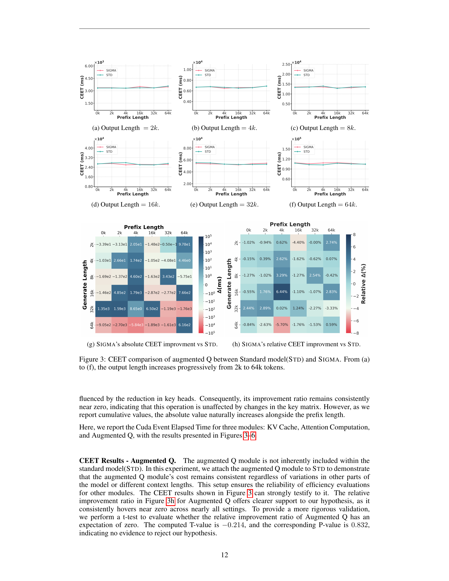
🔼 This figure compares the computational cost of the augmented Q module in the SIGMA model against a standard model (Std). The experiment is conducted across a range of output sequence lengths, from 2k tokens to 64k tokens. For each output length, the figure displays the computational time taken by both models. The x-axis represents the length of the input sequence (prefix length), and the y-axis represents the computational cost in milliseconds (CEET, Cuda Event Elapsed Time). This visualization helps to analyze the impact of the augmented Q module on the overall efficiency of the SIGMA model.
read the caption
Figure 3: CEET comparison of augmented Q between Standard model(Std) and Sigma. From (a) to (f), the output length increases progressively from 2k to 64k tokens.

🔼 This figure shows the results of the Kernel Execution Time (KET) test. Specifically, it displays a comparison of the time taken to execute the split kernel and combine kernel of the FlexHeadFA attention mechanism in the SIGMA model versus the standard model (STD). The x-axis represents the length of the input prefix, and the y-axis shows the time in nanoseconds. This test is designed to isolate and measure the efficiency of different parts of the attention computation. Multiple sub-figures are presented (a-c) showing the breakdown of the total kernel execution time into its component parts, allowing for a detailed analysis of the impact of SIGMA’s architecture changes on efficiency at varying sequence lengths.
read the caption
(a) Output Length =2kabsent2𝑘=2k= 2 italic_k.

🔼 The figure shows the Kernel Execution Time (KET) results for the combine kernel in the context of FlexHeadFA, comparing the performance between the standard model and SIGMA. The x-axis represents the prefix length (in tokens), and the y-axis represents the KET (in nanoseconds). The plot shows results for an output length of 4k tokens. This helps illustrate how the performance of the combine kernel changes with varying input sequence lengths for a specific output length. The goal is to assess the efficiency gains of SIGMA’s DiffQKV attention over the standard model.
read the caption
(b) Output Length =4kabsent4𝑘=4k= 4 italic_k.

🔼 This figure shows the results of measuring CUDA Event Elapsed Time (CEET) for different components of the attention mechanism in the SIGMA and Standard models. The x-axis represents the prefix length, and the y-axis represents the CEET in milliseconds. The output length is fixed at 8k tokens. The figure illustrates the differences in performance between SIGMA and Standard models across various prefix lengths.
read the caption
(c) Output Length =8kabsent8𝑘=8k= 8 italic_k.

🔼 This figure presents the results of the Cuda Event Elapsed Time (CEET) test, specifically focusing on scenarios with an output length of 16k tokens. It displays how the total computation time varies across different prefix lengths (the amount of input text preceding the generated text). The x-axis represents the prefix length, showing how computation time changes as more input is processed. The y-axis shows the CEET in milliseconds. The results likely compare the performance of the SIGMA model against a baseline model, showcasing the efficiency gains of SIGMA in long-context scenarios.
read the caption
(d) Output Length =16kabsent16𝑘=16k= 16 italic_k.

🔼 This figure shows the results of measuring CUDA event elapsed time (CEET) for different components of the SIGMA model. Specifically, it focuses on the scenario where the output length is 32k tokens. The x-axis represents the prefix length, and the y-axis represents the measured CEET. Different lines represent different modules within the model, such as KV cache, attention computation, and augmented Q. By comparing the CEET values for SIGMA and a standard model across various prefix lengths, the figure helps to illustrate the efficiency gains achieved by SIGMA, particularly in long-context scenarios.
read the caption
(e) Output Length =32kabsent32𝑘=32k= 32 italic_k.

🔼 This figure shows the results of the Cuda Event Elapsed Time (CEET) test with an output length of 64k tokens. The CEET test measures the total time elapsed for specific operations in the model. It is used to assess the efficiency of SIGMA and compare its performance against the standard model (STD). The x-axis represents the prefix length, and the y-axis represents the CEET in milliseconds. The figure displays the CEET for SIGMA and STD, allowing for a comparison of their efficiency across different prefix lengths. The results highlight the improvements in inference speed achieved by SIGMA, especially for longer sequences.
read the caption
(f) Output Length =64kabsent64𝑘=64k= 64 italic_k.

🔼 The figure shows the absolute improvement in Cuda Event Elapsed Time (CEET) achieved by SIGMA compared to the standard model (STD). It illustrates how much faster SIGMA is than the standard model in terms of milliseconds (ms). The improvement is shown across varying prefix and output lengths, revealing how the advantage of SIGMA changes across different text lengths.
read the caption
(g) Sigma’s absolute CEET improvment vs Std.

🔼 This figure shows the relative improvement in Cuda Event Elapsed Time (CEET) of SIGMA compared to the standard model (STD). The relative improvement is calculated as ((STD_CEET - SIGMA_CEET) / STD_CEET) * 100%. The x-axis represents different prefix lengths, and each subplot represents a different output length. The plot visually demonstrates how SIGMA’s efficiency gains increase as both prefix and output lengths increase. Specifically, it shows how much faster SIGMA is than STD in terms of time cost.
read the caption
(h) Sigma’s relative CEET improvment vs Std.

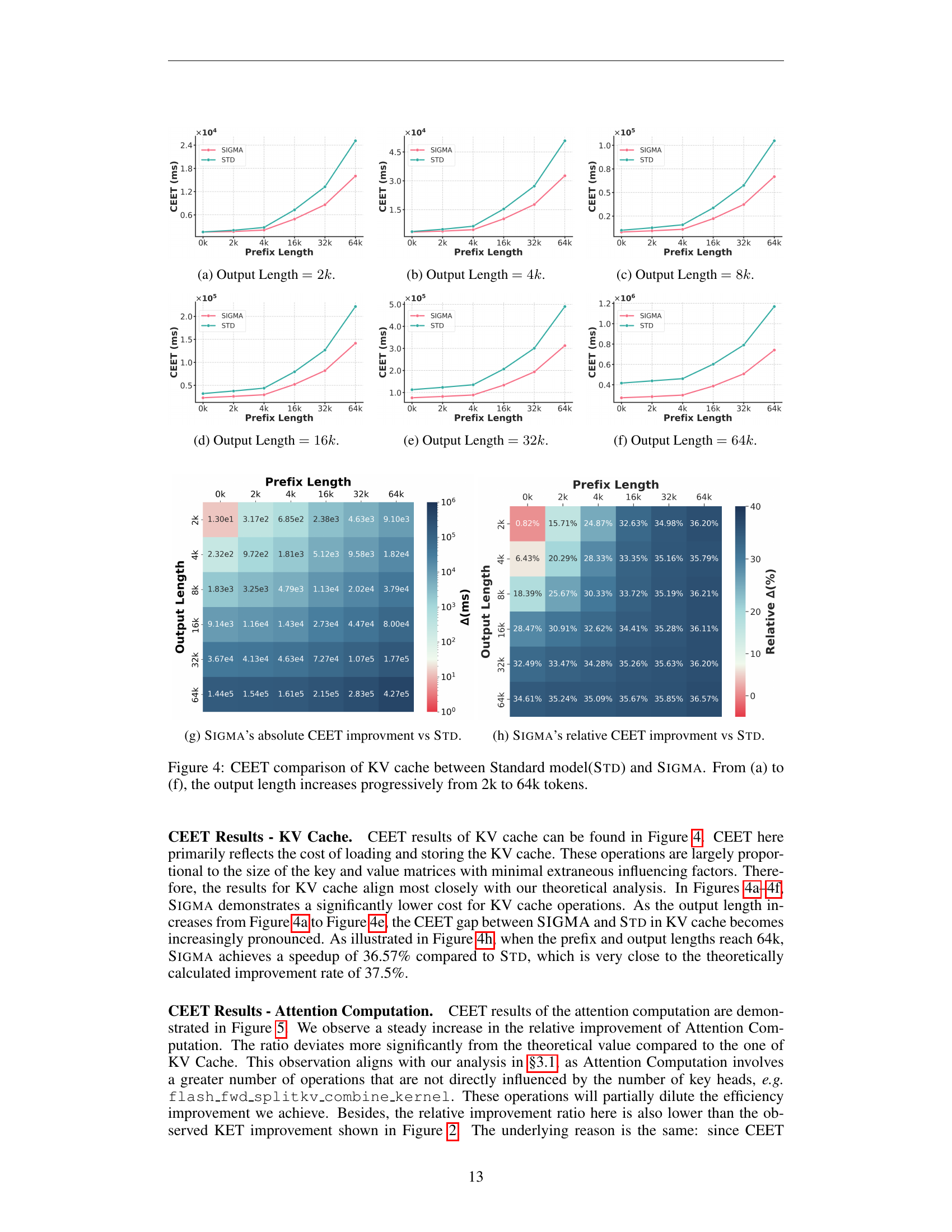
🔼 This figure compares the computational cost of loading and storing the key-value (KV) cache between the standard model (Std) and SIGMA, a novel language model introduced in the paper. The comparison is performed across varying output lengths, ranging from 2k to 64k tokens, and across different prefix lengths. The results are presented in a series of subplots, each showing the cost for a specific output length. This figure helps to illustrate the efficiency gains achieved by SIGMA through a reduction in the number of key heads, which directly impacts the size of the KV cache.
read the caption
Figure 4: CEET comparison of KV cache between Standard model(Std) and Sigma. From (a) to (f), the output length increases progressively from 2k to 64k tokens.

🔼 The figure shows the results of Kernel Execution Time (KET) measurements for the split and combine kernels of the FlexHeadFA attention mechanism. It compares the performance of the SIGMA model (with reduced key heads) against a standard model (STD) with balanced key and value heads. The x-axis represents the prefix length, and the y-axis displays the KET in nanoseconds. Separate graphs are presented for (a) the split kernel, (b) the combine kernel, and (c) the total KET which is sum of split and combine kernel.
read the caption
(a) Output Length =2kabsent2𝑘=2k= 2 italic_k.

🔼 The figure shows the result of Kernel Execution Time (KET) test, measuring the execution time of two kernels in the flash attention mechanism: the split kernel and the combine kernel. The test compares the performance between the standard model (STD) and SIGMA model, varying the prefix length while keeping the output length fixed at 4k tokens. The results illustrate the efficiency improvement of SIGMA over STD.
read the caption
(b) Output Length =4kabsent4𝑘=4k= 4 italic_k.

🔼 This figure shows the results of Kernel Execution Time (KET) test for the combine kernel in the DiffQKV attention mechanism. The x-axis represents the prefix length, and the y-axis represents the execution time in nanoseconds. There are two lines in the plot, one for SIGMA and another one for the standard model (STD). The output length is fixed at 8k tokens. The plot displays the execution time of the combine kernel as the prefix length varies. It’s used to evaluate the efficiency improvements brought by SIGMA, especially in long-sequence scenarios, by comparing the execution time with a standard model.
read the caption
(c) Output Length =8kabsent8𝑘=8k= 8 italic_k.

🔼 This figure is a part of the empirical analysis on efficiency. Specifically, it presents the Cuda Event Elapsed Time (CEET) results when the output length is 16k tokens. The x-axis represents the prefix length, and the y-axis represents the CEET in milliseconds. The plot shows the CEET for both SIGMA and the standard model (STD) to illustrate the efficiency improvement achieved by SIGMA. The results show that SIGMA is significantly more efficient than the STD in terms of inference time, especially for longer prefixes and sequences.
read the caption
(d) Output Length =16kabsent16𝑘=16k= 16 italic_k.

🔼 This figure presents the results of Cuda Event Elapsed Time (CEET) measurements for the ‘Attention Computation’ module in the SIGMA and STD models when the output length is 32k tokens. The x-axis represents the prefix length, and the y-axis displays the CEET in milliseconds. Separate lines show the results for the SIGMA and STD models, allowing comparison of their efficiency in processing different prefix lengths. The plot helps demonstrate the effect of the SIGMA model’s architecture, particularly its DiffQKV attention mechanism, on reducing computational time as prefix and sequence length increases.
read the caption
(e) Output Length =32kabsent32𝑘=32k= 32 italic_k.

🔼 This figure shows the results of the Cuda Event Elapsed Time (CEET) test when the output length is 64k tokens. The CEET test measures the total time taken for different operations within the attention mechanism (KV cache, attention computation, and augmented Q). By showing results for different prefix lengths (the amount of input text preceding the generation task), the plot helps to analyze how these operations’ time changes with both increasing input and output length.
read the caption
(f) Output Length =64kabsent64𝑘=64k= 64 italic_k.

🔼 The figure shows the absolute improvement in Cuda Event Elapsed Time (CEET) achieved by SIGMA compared to the standard model (STD). The x-axis represents the prefix length, while the y-axis shows the absolute difference in CEET (in milliseconds). Positive values indicate that SIGMA outperforms STD; and negative values indicate that STD outperforms SIGMA. The plot is further divided into subplots with different output lengths to illustrate how the performance gap changes as both the context and generated sequence length increase.
read the caption
(g) Sigma’s absolute CEET improvment vs Std.

🔼 This figure shows the relative improvement in Cuda Event Elapsed Time (CEET) of SIGMA compared to the standard model (STD). CEET measures the end-to-end time of specific operations. The relative improvement is calculated as the percentage decrease in CEET from STD to SIGMA. The figure likely displays this relative improvement across various conditions, such as different prefix and output sequence lengths, to illustrate how the performance gain changes under various scenarios.
read the caption
(h) Sigma’s relative CEET improvment vs Std.

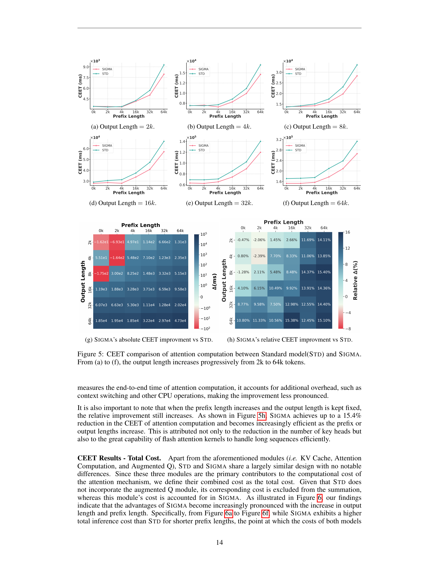
🔼 Figure 5 presents a comparison of the Cuda Event Elapsed Time (CEET) for the attention computation module between the Standard model (STD) and SIGMA across different output lengths. The x-axis represents the prefix length, while the y-axis shows the CEET in milliseconds. The figure is composed of six subfigures (a) through (f), each corresponding to a different output length, ranging from 2k to 64k tokens. Each subfigure contains two lines, one for SIGMA and one for STD, illustrating their respective computation times for the attention module. The results demonstrate that SIGMA exhibits superior efficiency compared to the STD, especially as the output and prefix lengths increase, which shows the effectiveness of the proposed DiffQKV attention module.
read the caption
Figure 5: CEET comparison of attention computation between Standard model(Std) and Sigma. From (a) to (f), the output length increases progressively from 2k to 64k tokens.

🔼 This figure shows the comparison of CUDA Event Elapsed Time (CEET) between SIGMA and the standard model (STD). The plots display the CEET for different prefix lengths (0k, 2k, 4k, 16k, 32k, 64k) when generating sequences of length 2k. This illustrates the relative performance of SIGMA in terms of inference speed across various sequence lengths and demonstrates the efficiency gains achieved by SIGMA, especially in longer sequences.
read the caption
(a) Output Length =2kabsent2𝑘=2k= 2 italic_k.

🔼 This figure shows the results of the Kernel Execution Time (KET) test for the combine kernel when the output sequence length is 4k tokens. The combine kernel combines output chunks generated during the flash attention calculation. The x-axis represents the prefix length (input sequence length), and the y-axis represents the execution time of the combine kernel. Separate lines show the results for the standard model (STD) and the SIGMA model.
read the caption
(b) Output Length =4kabsent4𝑘=4k= 4 italic_k.

🔼 The figure shows the results of the CUDA Event Elapsed Time (CEET) test for the attention computation. The CEET measures the total time spent on attention computation. The x-axis represents the prefix length, and the y-axis represents the CEET in milliseconds. The figure shows that the time spent on attention computation increases with the increase of the prefix length. This is expected as the attention mechanism needs to process more tokens as the prefix length increases. The figure also shows that the time spent on attention computation is longer when the output length is 8k compared to other output lengths. This is because the attention mechanism needs to compute attention scores between the query and key vectors for all the tokens, including those in the output sequence. The longer the output sequence, the more computations required, and thus the longer the computation time.
read the caption
(c) Output Length =8kabsent8𝑘=8k= 8 italic_k.

🔼 This figure shows the results of measuring CUDA event elapsed time (CEET). Specifically, it displays the CEET for different prefix lengths when the output length is fixed at 16k tokens. The results are relevant to the efficiency analysis of the SIGMA model and highlight the impact of varying prefix lengths on overall processing time.
read the caption
(d) Output Length =16kabsent16𝑘=16k= 16 italic_k.

🔼 This figure shows the results from the Cuda Event Elapsed Time (CEET) test, specifically focusing on the scenario where the output length is 32k tokens. The test measures the time taken for different stages of the attention mechanism: KV Cache (loading and storing key and value vectors), Attention Computation (calculating attention scores and weighted sums), and Augmented Q (applying a modified query component). By comparing the time taken for these stages between the SIGMA and Standard models across varying prefix lengths, the figure illustrates the efficiency gains achieved by SIGMA, particularly in long-context scenarios.
read the caption
(e) Output Length =32kabsent32𝑘=32k= 32 italic_k.

🔼 This figure shows the results of measuring the total cost of CUDA events elapsed time (CEET) for different prefix and output lengths when the output length is set to 64k tokens. The x-axis represents the prefix length, and the y-axis shows the CEET in milliseconds. The plot contains two lines: one for the standard model (STD) and one for SIGMA. The figure illustrates the efficiency gains of SIGMA compared to the standard model, especially as the context length increases.
read the caption
(f) Output Length =64kabsent64𝑘=64k= 64 italic_k.

🔼 The figure shows the absolute improvement in CUDA Event Elapsed Time (CEET) of SIGMA compared to the standard model (STD). The improvement is calculated by subtracting the CEET of STD from that of SIGMA for different combinations of prefix and output lengths. Positive values indicate that SIGMA is faster; negative values indicate that SIGMA is slower. The x-axis represents the prefix length, and the y-axis shows the difference in CEET.
read the caption
(g) Sigma’s absolute CEET improvment vs Std.

🔼 This figure shows the relative improvement in CUDA Event Elapsed Time (CEET) achieved by SIGMA compared to the standard model (STD). The relative improvement is calculated as ((STD CEET - SIGMA CEET) / STD CEET) * 100. The figure likely displays this relative improvement across various experimental conditions, such as different sequence lengths of the input and output texts. It helps to visualize the efficiency gains of SIGMA, particularly in scenarios with longer sequences, where the improvements are expected to be more substantial. The y-axis represents the relative improvement in percentage, and the x-axis likely represents the different experimental conditions.
read the caption
(h) Sigma’s relative CEET improvment vs Std.

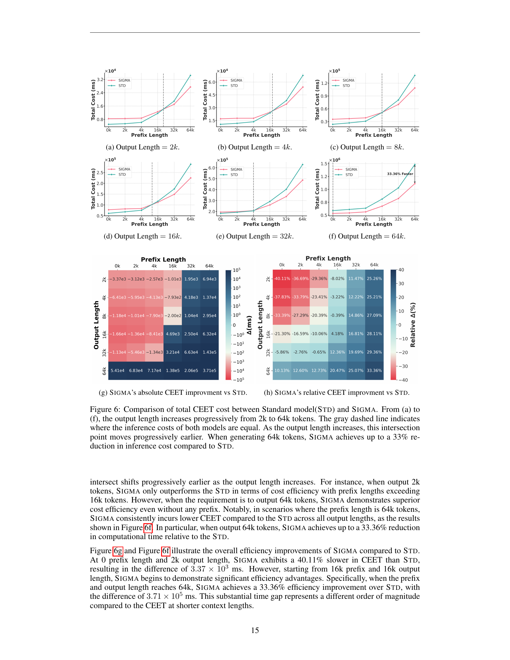
🔼 Figure 6 presents a comparison of the total computational cost (measured using CUDA Event Elapsed Time, or CEET) between the standard model (Std) and the SIGMA model for varying output lengths. The x-axis represents the prefix length, and the y-axis displays the total CEET. Subplots (a) through (f) show results for output lengths increasing from 2k to 64k tokens. A gray dashed line in each plot indicates the point where the computational costs of both models are equal. As the output length increases, this intersection point shifts left, indicating that SIGMA’s efficiency advantage increases significantly for longer outputs. For an output length of 64k tokens, SIGMA demonstrates a cost reduction of up to 33% when compared to the standard model. This illustrates the substantial efficiency gains of the SIGMA model, particularly in long-context scenarios, and validates the theoretical analysis presented earlier in the paper.
read the caption
Figure 6: Comparison of total CEET cost between Standard model(Std) and Sigma. From (a) to (f), the output length increases progressively from 2k to 64k tokens. The gray dashed line indicates where the inference costs of both models are equal. As the output length increases, this intersection point moves progressively earlier. When generating 64k tokens, Sigma achieves up to a 33% reduction in inference cost compared to Std.
More on tables
| Model | Overall | Commonsense & Comprehension | Continued | LM | ||||||
| Hella. | ObQA | Wino. | ARC. | PIQA | SciQ | Bool. | Logi. | LAMB. | ||
| MHA (==32) | 52.40 | 55.6 | 37.6 | 57.6 | 36.0 | 73.9 | 85.5 | 59.6 | 28.9 | 36.8 |
| w/ Half K Dim. | 52.56 (0.16) | 55.2 | 39.4 | 56.9 | 36.9 | 72.7 | 84.1 | 63.3 | 27.8 | 36.8 |
| GQA (==16) | 52.14 | 55.1 | 39.6 | 56.3 | 35.4 | 71.9 | 85.0 | 61.4 | 27.8 | 36.8 |
| w/ Half K Dim. | 52.06 (0.08) | 54.3 | 39.8 | 56.9 | 36.7 | 72.0 | 83.9 | 59.5 | 29.2 | 36.2 |
| GQA (==4) | 51.66 | 54.0 | 38.0 | 56.0 | 37.5 | 72.3 | 82.0 | 61.3 | 28.6 | 35.4 |
| w/ Half K Dim. | 51.92 (0.26) | 53.4 | 39.2 | 56.6 | 35.6 | 72.5 | 84.0 | 62.3 | 28.9 | 34.8 |
🔼 This table presents an ablation study investigating the impact of halving the Key (K) head dimension on the model’s performance. It explores the trade-off between inference efficiency (achieved by reducing the size of the Key-Value (KV) cache) and the potential compromise in accuracy. The study maintains a consistent number of Query (Q) heads (32) across all model variations to isolate the effect of the K head dimension change. The results demonstrate that reducing the K head dimension significantly improves inference speed without substantially affecting overall performance.
read the caption
Table 2: The ablation studies of halving the K head dimension. The results indicate that this adjustment, while largely improving the inference efficiency by reducing the size of KV cache, does not significantly compromise performance. The number of Q heads is 32 for all models (nqh=32superscriptsubscript𝑛𝑞ℎ32n_{q}^{h}=32italic_n start_POSTSUBSCRIPT italic_q end_POSTSUBSCRIPT start_POSTSUPERSCRIPT italic_h end_POSTSUPERSCRIPT = 32).
| Model | Overall | Commonsense & Comprehension | Continued | LM | ||||||
| Hella. | ObQA | Wino. | ARC. | PIQA | SciQ | Bool. | Logi. | LAMB. | ||
| MHA (==32) | 52.40 | 55.6 | 37.6 | 57.6 | 36.0 | 73.9 | 85.5 | 59.6 | 28.9 | 36.8 |
| + Sel.V-top100 | 52.10 (0.30) | 55.6 | 37.6 | 57.6 | 36.0 | 74.0 | 84.8 | 59.3 | 27.0 | 36.9 |
| GQA (==16) | 52.14 | 55.1 | 39.6 | 56.3 | 35.4 | 71.9 | 85.0 | 61.4 | 27.8 | 36.8 |
| + Sel.V-top100 | 52.08 (0.06) | 55.2 | 39.6 | 56.3 | 35.4 | 71.8 | 84.4 | 61.6 | 27.8 | 36.7 |
| GQA (==4) | 51.66 | 54.0 | 38.0 | 56.0 | 37.5 | 72.3 | 82.0 | 61.3 | 28.6 | 35.4 |
| + Sel.V-top100 | 51.67 (0.01) | 54.0 | 38.2 | 55.9 | 37.5 | 72.2 | 82.0 | 61.2 | 28.6 | 35.4 |
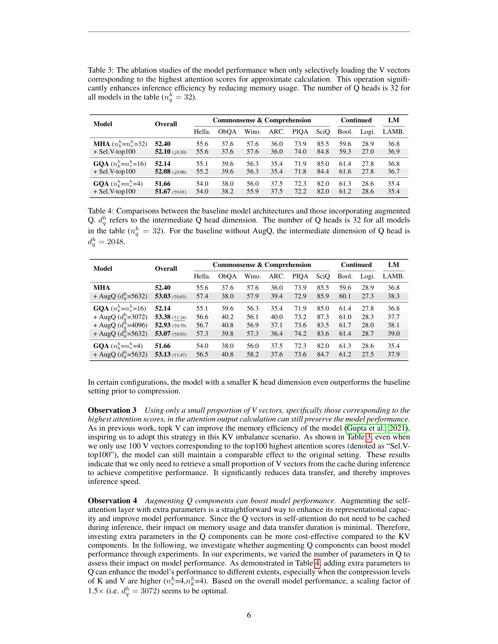
🔼 This table presents the results of ablation studies conducted to evaluate the impact of selectively loading only the top V vectors (those with the highest attention scores) during approximate calculations within the attention mechanism. The goal was to assess the trade-off between model performance and inference efficiency by reducing memory usage. The number of query heads (Q) was held constant at 32 across all model variations in this experiment.
read the caption
Table 3: The ablation studies of the model performance when only selectively loading the V vectors corresponding to the highest attention scores for approximate calculation. This operation significantly enhances inference efficiency by reducing memory usage. The number of Q heads is 32 for all models in the table (nqh=32superscriptsubscript𝑛𝑞ℎ32n_{q}^{h}=32italic_n start_POSTSUBSCRIPT italic_q end_POSTSUBSCRIPT start_POSTSUPERSCRIPT italic_h end_POSTSUPERSCRIPT = 32).
| Model | Overall | Commonsense & Comprehension | Continued | LM | ||||||
| Hella. | ObQA | Wino. | ARC. | PIQA | SciQ | Bool. | Logi. | LAMB. | ||
| MHA | 52.40 | 55.6 | 37.6 | 57.6 | 36.0 | 73.9 | 85.5 | 59.6 | 28.9 | 36.8 |
| + AugQ (=5632) | 53.03 (0.63) | 57.4 | 38.0 | 57.9 | 39.4 | 72.9 | 85.9 | 60.1 | 27.3 | 38.3 |
| GQA (==16) | 52.14 | 55.1 | 39.6 | 56.3 | 35.4 | 71.9 | 85.0 | 61.4 | 27.8 | 36.8 |
| + AugQ (=3072) | 53.38 (1.24) | 56.6 | 40.2 | 56.1 | 40.0 | 73.2 | 87.3 | 61.0 | 28.3 | 37.7 |
| + AugQ (=4096) | 52.93 (0.79) | 56.7 | 40.8 | 56.9 | 37.1 | 73.6 | 83.5 | 61.7 | 28.0 | 38.1 |
| + AugQ (=5632) | 53.07 (0.93) | 57.3 | 39.8 | 57.3 | 36.4 | 74.2 | 83.6 | 61.4 | 28.7 | 39.0 |
| GQA (==4) | 51.66 | 54.0 | 38.0 | 56.0 | 37.5 | 72.3 | 82.0 | 61.3 | 28.6 | 35.4 |
| + AugQ (=5632) | 53.13 (1.47) | 56.5 | 40.8 | 58.2 | 37.6 | 73.6 | 84.7 | 61.2 | 27.5 | 37.9 |
🔼 Table 4 presents an ablation study comparing the performance of models with and without an augmented query (AugQ) component. It investigates the impact of increasing the intermediate dimension of the query head (dqh) on overall model performance. The study uses a consistent number of 32 query heads (nqh=32) across all model variations. The baseline models have an intermediate query head dimension of 2048 (dqh=2048). The table compares various models with different augmented Q head dimensions to show the impact of increased model parameters only in the query part. The performance is measured on various downstream tasks.
read the caption
Table 4: Comparisons between the baseline model architectures and those incorporating augmented Q. dqhsuperscriptsubscript𝑑𝑞ℎd_{q}^{h}italic_d start_POSTSUBSCRIPT italic_q end_POSTSUBSCRIPT start_POSTSUPERSCRIPT italic_h end_POSTSUPERSCRIPT refers to the intermediate Q head dimension. The number of Q heads is 32 for all models in the table (nqh=32superscriptsubscript𝑛𝑞ℎ32n_{q}^{h}=32italic_n start_POSTSUBSCRIPT italic_q end_POSTSUBSCRIPT start_POSTSUPERSCRIPT italic_h end_POSTSUPERSCRIPT = 32). For the baseline without AugQ, the intermediate dimension of Q head is dqh=2048superscriptsubscript𝑑𝑞ℎ2048d_{q}^{h}=2048italic_d start_POSTSUBSCRIPT italic_q end_POSTSUBSCRIPT start_POSTSUPERSCRIPT italic_h end_POSTSUPERSCRIPT = 2048.
| Model | Overall | Commonsense & Comprehension | Continued | LM | ||||||
| Hella. | ObQA | Wino. | ARC. | PIQA | SciQ | Bool. | Logi. | LAMB. | ||
| GQA | 52.14 | 55.1 | 39.6 | 56.3 | 35.4 | 71.9 | 85.0 | 61.4 | 27.8 | 36.8 |
| + AugF (=) | 53.26 (1.12) | 57.6 | 39.6 | 57.3 | 38.5 | 73.2 | 87.3 | 59.0 | 27.6 | 39.2 |
| + AugQ (=) | 53.38 (1.24) | 56.6 | 40.2 | 56.1 | 40.0 | 73.2 | 87.3 | 61.0 | 28.3 | 37.7 |
| + AugF (=) | 53.16 (1.02) | 59.3 | 40.0 | 57.0 | 38.3 | 73.9 | 85.2 | 59.8 | 24.9 | 40.1 |
| + AugF (=) & AugQ (=) | 54.55 (2.41) | 58.8 | 41.8 | 57.5 | 39.7 | 74.4 | 86.9 | 62.4 | 28.1 | 41.5 |
| + AugF (=) | 54.50 (2.36) | 60.5 | 42.4 | 59.8 | 39.8 | 74.7 | 87.3 | 59.9 | 27.0 | 39.2 |
| + AugF (=) & AugQ (=) | 54.67 (2.53) | 60.5 | 41.6 | 57.4 | 39.9 | 74.7 | 87.3 | 59.6 | 27.3 | 43.8 |
| + AugF (=) | 55.08 (2.94) | 62.4 | 41.4 | 57.3 | 41.3 | 75.3 | 88.3 | 60.6 | 26.6 | 42.5 |
| + AugF (=) & AugQ (=) | 55.09 (2.95) | 61.6 | 39.8 | 61.0 | 40.5 | 75.1 | 88.7 | 59.6 | 28.3 | 41.2 |
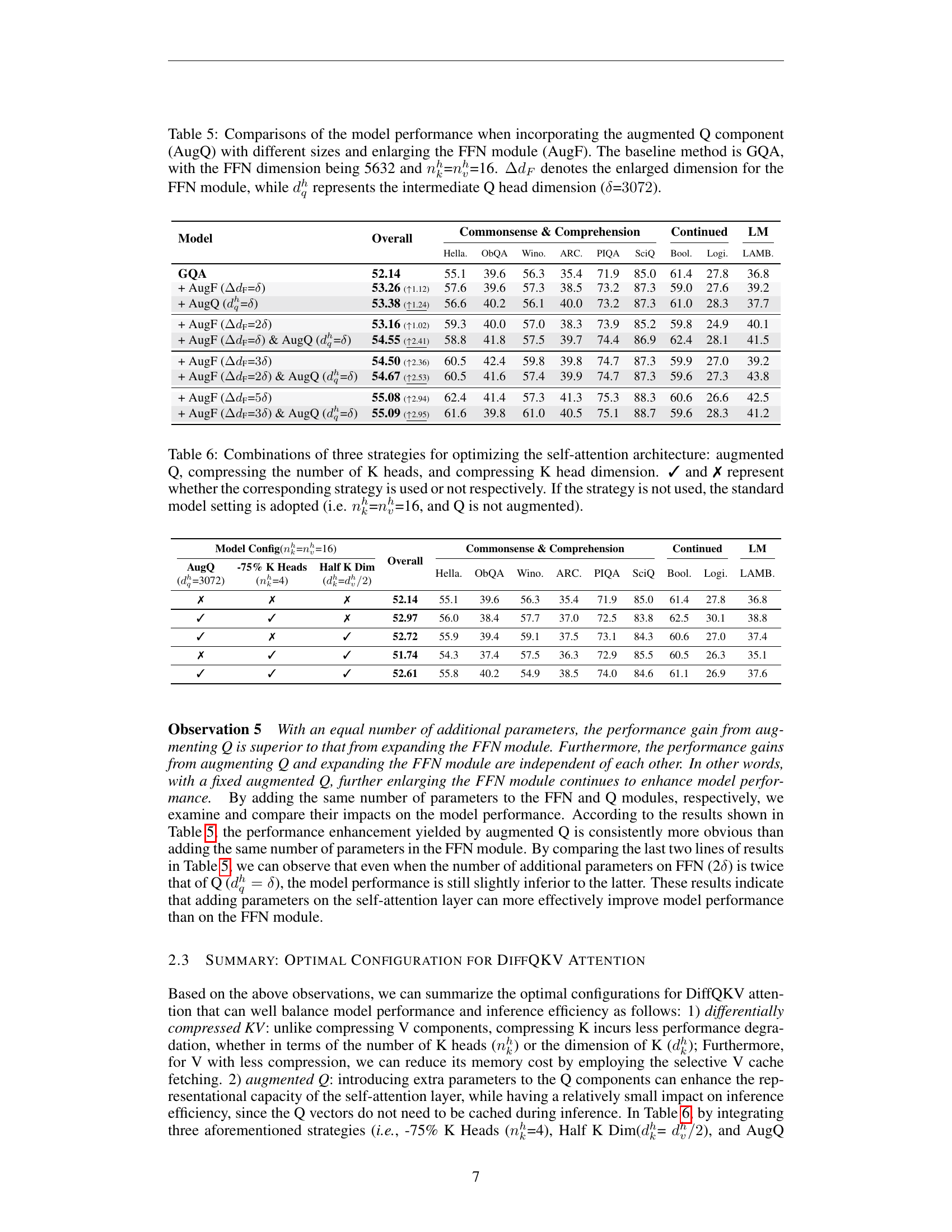
🔼 This table presents the results of ablation studies on the SIGMA model, investigating the impact of incorporating an augmented query (Q) component and enlarging the feed-forward network (FFN) module on model performance. The baseline model used is Grouped-Query Attention (GQA) with an FFN dimension of 5632 and an equal number of key and value heads (both set to 16). The experiments systematically vary the size of the augmented Q component (denoted as dqh) and the FFN module’s enlarged dimension (denoted as ΔdF). The table shows how these modifications affect overall model performance as measured on various tasks.
read the caption
Table 5: Comparisons of the model performance when incorporating the augmented Q component (AugQ) with different sizes and enlarging the FFN module (AugF). The baseline method is GQA, with the FFN dimension being 5632 and nkhsuperscriptsubscript𝑛𝑘ℎn_{k}^{h}italic_n start_POSTSUBSCRIPT italic_k end_POSTSUBSCRIPT start_POSTSUPERSCRIPT italic_h end_POSTSUPERSCRIPT=nvhsuperscriptsubscript𝑛𝑣ℎn_{v}^{h}italic_n start_POSTSUBSCRIPT italic_v end_POSTSUBSCRIPT start_POSTSUPERSCRIPT italic_h end_POSTSUPERSCRIPT=16. ΔdFΔsubscript𝑑𝐹\Delta d_{F}roman_Δ italic_d start_POSTSUBSCRIPT italic_F end_POSTSUBSCRIPT denotes the enlarged dimension for the FFN module, while dqhsuperscriptsubscript𝑑𝑞ℎd_{q}^{h}italic_d start_POSTSUBSCRIPT italic_q end_POSTSUBSCRIPT start_POSTSUPERSCRIPT italic_h end_POSTSUPERSCRIPT represents the intermediate Q head dimension (δ𝛿\deltaitalic_δ=3072307230723072).
| Model Config(==16) | Overall | Commonsense & Comprehension | Continued | LM | ||||||||
| AugQ | -75% K Heads | Half K Dim | Hella. | ObQA | Wino. | ARC. | PIQA | SciQ | Bool. | Logi. | LAMB. | |
| (=3072) | (=4) | (=) | ||||||||||
| ✗ | ✗ | ✗ | 52.14 | 55.1 | 39.6 | 56.3 | 35.4 | 71.9 | 85.0 | 61.4 | 27.8 | 36.8 |
| ✓ | ✓ | ✗ | 52.97 | 56.0 | 38.4 | 57.7 | 37.0 | 72.5 | 83.8 | 62.5 | 30.1 | 38.8 |
| ✓ | ✗ | ✓ | 52.72 | 55.9 | 39.4 | 59.1 | 37.5 | 73.1 | 84.3 | 60.6 | 27.0 | 37.4 |
| ✗ | ✓ | ✓ | 51.74 | 54.3 | 37.4 | 57.5 | 36.3 | 72.9 | 85.5 | 60.5 | 26.3 | 35.1 |
| ✓ | ✓ | ✓ | 52.61 | 55.8 | 40.2 | 54.9 | 38.5 | 74.0 | 84.6 | 61.1 | 26.9 | 37.6 |
🔼 Table 6 presents an ablation study on three different optimization strategies applied to the self-attention mechanism of a language model. The strategies are: augmenting the query (Q) component by increasing its dimensionality; reducing the number of key (K) heads; and reducing the dimensionality of the key heads. The table shows the model’s performance across various metrics, depending on which combinations of these three strategies are used. A checkmark (✓) indicates that a strategy was used, while an X (✗) indicates it wasn’t. The baseline model configuration (when none of the three strategies are applied) uses the same number of key and value heads (16), with no augmentation of the query component.
read the caption
Table 6: Combinations of three strategies for optimizing the self-attention architecture: augmented Q, compressing the number of K heads, and compressing K head dimension. ✓ and ✗ represent whether the corresponding strategy is used or not respectively. If the strategy is not used, the standard model setting is adopted (i.e. nkhsuperscriptsubscript𝑛𝑘ℎn_{k}^{h}italic_n start_POSTSUBSCRIPT italic_k end_POSTSUBSCRIPT start_POSTSUPERSCRIPT italic_h end_POSTSUPERSCRIPT=nvhsuperscriptsubscript𝑛𝑣ℎn_{v}^{h}italic_n start_POSTSUBSCRIPT italic_v end_POSTSUBSCRIPT start_POSTSUPERSCRIPT italic_h end_POSTSUPERSCRIPT=16, and Q is not augmented).
| Parameter Scale | 1.5B | 10B |
| Layers | 26 | 32 |
| Hidden Dimension | 2,048 | 4,096 |
| FFN Dimension | 6,144 | 14,336 |
| Aug Q Dimension | 3,072 | 6,144 |
| Attention Heads | 32 | 32 |
| Key Heads | 4 | 4 |
| Value Heads | 16 | 16 |
| Peak Learning Rate | 4.0e-4 | 1.5e-4 |
| Activation Function | SwiGLU | SwiGLU |
| Vocabulary Size | 128,256 | 128,256 |
| Positional Embeddings | ROPE (50,000) | ROPE (500,000) |
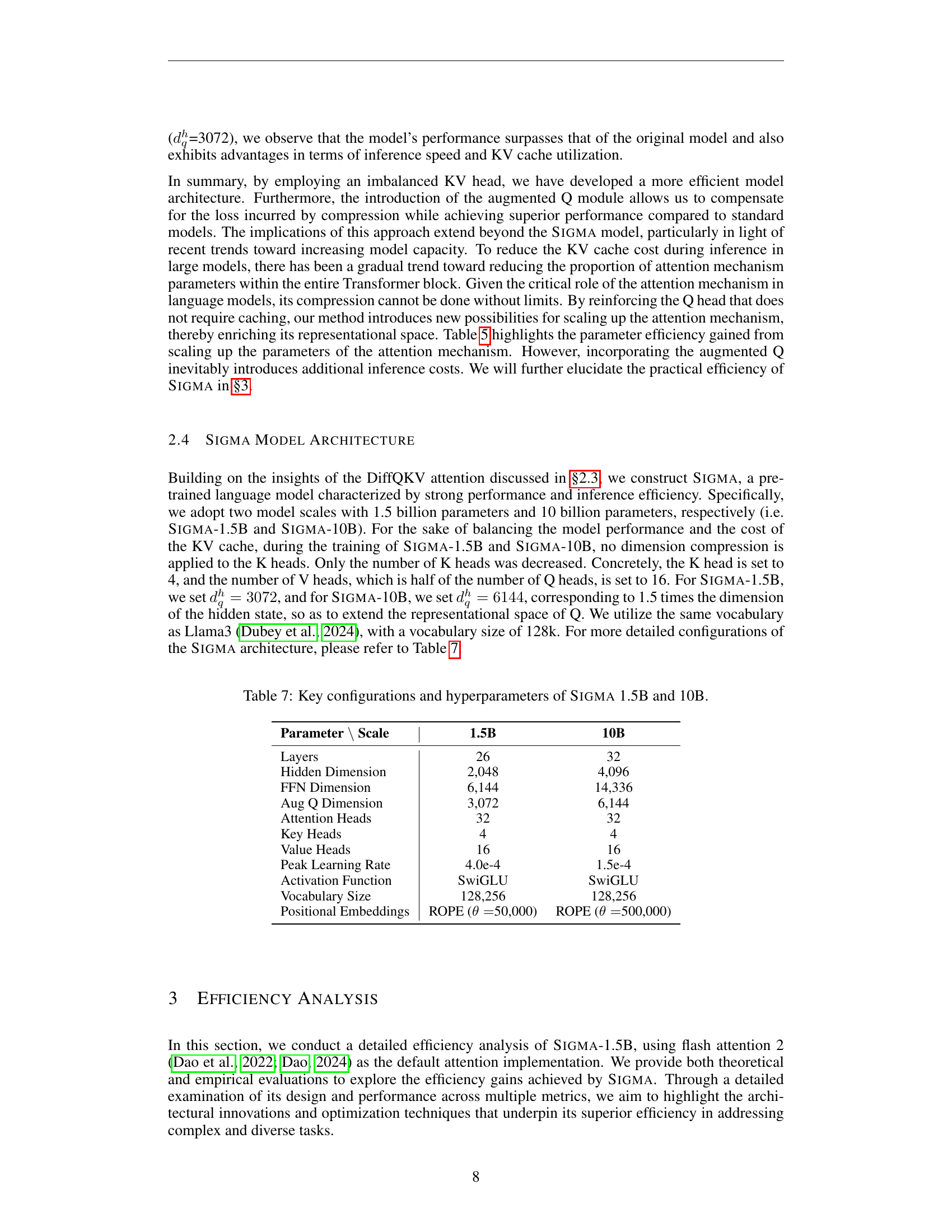
🔼 This table details the key architectural configurations and hyperparameters of the two SIGMA models: SIGMA 1.5B and SIGMA 10B. It provides a comprehensive overview of the models’ specifications, including the number of layers, hidden dimension, FFN (Feed-Forward Network) dimension, augmented Q dimension, attention heads, key heads, value heads, peak learning rate, activation function, and vocabulary size. This information is crucial for understanding the design choices and the resulting performance of each model.
read the caption
Table 7: Key configurations and hyperparameters of Sigma 1.5B and 10B.
| Prefix | Std | Sigma 1.5B | Relative Improvement | ||||||
| Length | Split | Combine | Total Cost | Split | Combine | Total Cost | Split | Combine | Total Cost |
| 2k | 2.53E+6 | 1.88E+6 | 4.41E+6 | 2.50E+6 | 1.85E+6 | 4.34E+6 | 1.17% | 1.68% | 1.39% |
| 4k | 4.68E+6 | 1.91E+6 | 6.59E+6 | 3.49E+6 | 1.91E+6 | 5.40E+6 | 25.33% | 0.08% | 18.02% |
| 16k | 1.52E+7 | 1.94E+6 | 1.72E+7 | 1.12E+7 | 1.94E+6 | 1.31E+7 | 26.30% | 0.25% | 23.35% |
| 32k | 2.75E+7 | 1.99E+6 | 2.95E+7 | 2.00E+7 | 2.01E+6 | 2.21E+7 | 27.21% | -0.93% | 25.31% |
🔼 This table presents the Kernel Execution Time (KET) results in nanoseconds (ns) for different prefix lengths, ranging from 2,000 to 32,000 tokens. The output length is kept constant at 10 tokens. The KET is broken down into two key components: the ‘Split’ kernel and the ‘Combine’ kernel, which represent different stages of the flash attention mechanism. The table compares the performance of the SIGMA model (a proposed model in the paper) with that of a standard model (STD) for each prefix length, highlighting the improvements in efficiency achieved by SIGMA.
read the caption
Table 8: KET Results (ns) with the prefix length increase from 2k to 32k, keeping the output length as 10. Split represents the split kernel and Combine represents the combine kernel.
| Data Type | Sources | Size | # Tokens |
| General System | CCF Ranking list | 14.0 G | 3.3 B |
| arXiv | 33.0 G | 5.4 B | |
| Design Capability | Technical blogs & Developer forums | 14.5 G | 3.2 B |
| Debug Capability | Stack Overflow | 38.9 G | 7.6 B |
🔼 Table 9 shows the composition of the system domain pre-training data used for training the SIGMA language model. It breaks down the data by type (General System, Design Capability, Debug Capability), source (e.g., CCF Ranking list, arXiv, Stack Overflow), size (in gigabytes), and number of tokens (in billions). This provides a detailed view of the data sources and their relative proportions used in SIGMA’s pre-training, showing the emphasis placed on system-specific data in its training regime.
read the caption
Table 9: Composition of the system domain pre-training data for Sigma.
| Model |
|
|
|
|
| Accuracy | ||||||||||
| GPT-3.5 | 70.0 | 36.0 | 21.0 | 6.0 | 11.0 | 13.0 | ||||||||||
| GPT-4 | 84.0 | 61.0 | 62.0 | 13.0 | 21.0 | 25.0 | ||||||||||
| Mistral-7B-S | 80.6 | 58.7 | 62.0 | 24.9 | 19.0 | 30.7 | ||||||||||
| Mistral-7B-P-S | 83.4 | 65.3 | 66.3 | 23.9 | 21.5 | 32.2 | ||||||||||
| Llama3-8B-S | 86.4 | 69.1 | 64.4 | 42.0 | 32.7 | 50.7 | ||||||||||
| Llama3-8B-P-S | 87.5 | 72.2 | 69.3 | 46.3 | 37.1 | 57.1 | ||||||||||
| Codegemma-7B-P-S | 84.2 | 61.8 | 65.9 | 23.9 | 21.0 | 32.7 | ||||||||||
| Starcoder2-7B-P-S | 86.5 | 66.5 | 64.9 | 31.2 | 23.4 | 38.1 | ||||||||||
| DeepSeekCoder1.5-7B-P-S | 86.3 | 68.4 | 63.9 | 41.0 | 30.7 | 49.3 | ||||||||||
| Gemma2-9B-P-S | 90.3 | 72.2 | 78.1 | 34.2 | 26.8 | 43.9 | ||||||||||
| Sigma-System-10B | 87.5 | 80.9 | 78.0 | 57.0 | 74.0 | 74.5 |
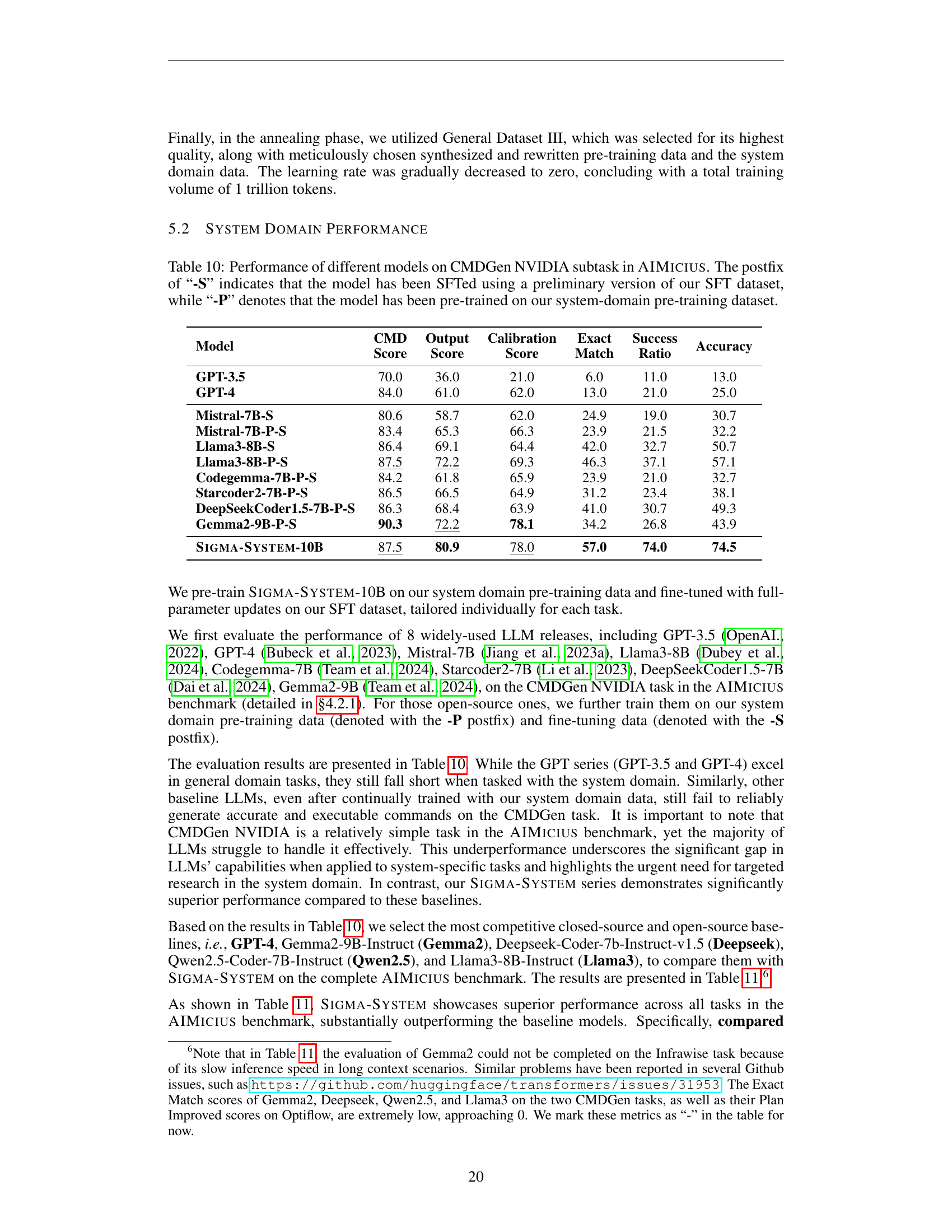
🔼 This table compares the performance of various large language models (LLMs) on the CMDGen NVIDIA subtask within the AIMICIUS benchmark. The CMDGen task focuses on generating GPU-related commands. The NVIDIA subtask specifically targets commands for NVIDIA GPUs. The table shows several metrics for each model, including the CMD Score (cosine similarity between generated and ground-truth commands), Output Score (cosine similarity of execution results), Calibration Score (accuracy measure), Exact Match (exact command match), Success Ratio (similar enough execution results), and Accuracy (overall accuracy). The models are grouped and categorized, with the postfix ‘-S’ indicating fine-tuning (SFT) with a preliminary version of the authors’ dataset, and ‘-P’ indicating pre-training on the authors’ system-domain dataset. This allows for a comparison of the impact of different training methods and datasets on the models’ performance on this specific task.
read the caption
Table 10: Performance of different models on CMDGen NVIDIA subtask in AIMicius. The postfix of “-S” indicates that the model has been SFTed using a preliminary version of our SFT dataset, while “-P” denotes that the model has been pre-trained on our system-domain pre-training dataset.
| CMD |
| Score |
🔼 This table presents a comprehensive comparison of the performance of various large language models (LLMs) on the AIMICIUS benchmark, a newly proposed evaluation suite specifically designed for system domain tasks. The models compared include SIGMA-SYSTEM 10B (a fine-tuned version of the SIGMA model using a proprietary dataset), as well as several established baselines: GPT-4, Gemma2-9B-Instruct, Deepseek-Coder-7b-Instruct-v1.5, Qwen2.5-Coder-7B-Instruct, and Llama3-8B-Instruct. The table evaluates performance across multiple tasks within the AIMICIUS benchmark, with metrics normalized to a 0-100 scale for easier comparison. The most crucial metrics for each task are highlighted in bold. The results provide insights into the relative strengths and weaknesses of each model in handling the complexities of system-related tasks.
read the caption
Table 11: Evaluation results on the AIMicius benchmark. The baselines include GPT-4, Gemma2-9B-Instruct, Deepseek-Coder-7b-Instruct-v1.5, Qwen2.5-Coder-7B-Instruct, and Llama3-8B-Instruct. All metrics are normalized to a scale of 0 to 100, with higher values indicating better performance. Bolded metrics represent the most critical evaluation criteria for each task. Sigma-System 10B is fine-tuned (SFT) using our proprietary dataset.
| Output |
| Score |
🔼 This table presents a comparison of the performance of SIGMA-1.5B against several other state-of-the-art language models on various commonsense reasoning and text understanding benchmarks. The results are obtained using zero-shot prompting, and the table shows the performance on each benchmark, reported as an average score across multiple metrics. Note that the authors re-evaluated the baseline models to ensure fair comparisons and consistency; therefore, the values may slightly differ from the original reports of the baseline models.
read the caption
Table 12: Comparisons with baseline models on commonsense reasoning and text understanding tasks. Differences with original reports in the baseline models are due to our unified re-evaluations for fair comparisons.
| Calibration |
| Score |
🔼 This table compares the performance of the SIGMA-1.5B model against several other state-of-the-art models on various general, coding, and mathematical problem-solving tasks. The metrics evaluated include performance on the MMLU, MMLU-Pro, and BBH general problem-solving benchmarks; HumanEval and MBPP code generation benchmarks; and MATH and GSM8K math problem-solving benchmarks. The results are presented to highlight SIGMA-1.5B’s performance relative to other models with comparable parameter sizes, offering insight into its capabilities across different task domains. Note that differences from previously published results for the baseline models are due to the authors’ consistent re-evaluation process for fair comparisons.
read the caption
Table 13: Comparisons with baseline models on general, coding, and math problem-solving tasks. Differences with original reports in the baseline models are due to our unified re-evaluations for fair comparisons.
Full paper#