TL;DR#
Mobile applications demand lightweight, fast, and accurate vision models. Current convolutional neural networks (CNNs) excel in speed but lack the global context modeling of vision transformers (ViTs), which are too computationally expensive for mobile deployment. Hybrid approaches attempt to bridge this gap, but often compromise either speed or accuracy.
This research introduces iFormer, a new hybrid network architecture that overcomes these limitations. It leverages the strengths of both CNNs (ConvNeXt specifically) and ViTs, but with a crucial improvement: a novel single-head modulation attention mechanism significantly reduces the computational cost of self-attention. Extensive experiments demonstrate iFormer’s superiority over existing mobile models in both accuracy and speed across various image classification, detection, and segmentation tasks, proving its efficiency and effectiveness in real-world mobile applications.
Key Takeaways#
Why does it matter?#
This paper is important because it presents iFormer, a novel family of mobile hybrid vision networks that achieves a state-of-the-art balance between speed and accuracy. It addresses the challenges of deploying computationally expensive vision transformers on mobile devices by integrating efficient convolutional operations and a novel single-head modulation attention mechanism. This work is relevant to the current trends in lightweight deep learning and mobile computer vision, opening avenues for research into more efficient and effective hybrid neural network architectures.
Visual Insights#

🔼 This figure compares the latency and accuracy of various lightweight neural networks, including the novel iFormer model, on the ImageNet-1k image classification benchmark. The latency is measured using an iPhone 13, providing a real-world performance metric relevant to mobile applications. The results show iFormer achieving a superior balance between low latency and high accuracy compared to other state-of-the-art models, demonstrating its Pareto optimality (meaning improvements in latency cannot be made without sacrificing accuracy, and vice versa).
read the caption
Figure 1: Comparison of latency and accuracy between our iFormer and other existing methods on ImageNet-1k. The latency is measured on an iPhone 13. Our iFormer is Pareto-optimal.
| Models | Latency (ms) | Top-1 Acc. (%) |
| MHA Baseline | 1.40 | 79.9 |
| SHA Baseline | 1.12 (1.25) | 79.8 |
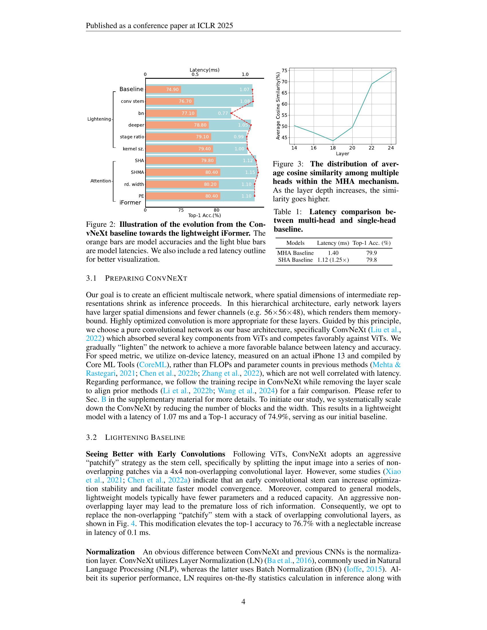
🔼 This table compares the latency and Top-1 accuracy of two baseline models: one using multi-head self-attention (MHA) and the other using single-head self-attention (SHA). It highlights the significant reduction in latency achieved by using SHA while maintaining comparable accuracy, demonstrating the efficiency of the proposed single-head approach for mobile applications.
read the caption
Table 1: Latency comparison between multi-head and single-head baseline.
In-depth insights#
MobileNet Enhancements#
MobileNet enhancements predominantly focus on improving efficiency and accuracy. Strategies include architectural modifications, such as inverted residual blocks and depthwise separable convolutions, to reduce computational cost. Channel pruning and knowledge distillation are employed to compress model size and improve generalization. Attention mechanisms, inspired by Transformers, are incorporated to capture longer-range dependencies, often leading to gains in accuracy. The integration of these methods aims for real-time performance on resource-constrained mobile devices, balancing accuracy and efficiency, while addressing challenges like high memory usage and latency.
Hybrid Network Design#
Hybrid network design, integrating Convolutional Neural Networks (CNNs) and Vision Transformers (ViTs), is a promising area for improving model performance. CNNs excel at local feature extraction, while ViTs effectively capture global context. The challenge lies in combining these strengths efficiently, especially for mobile applications where latency is critical. Effective hybrid designs often involve a hierarchical structure, leveraging CNNs’ efficiency in earlier stages for feature extraction, and then progressively incorporating ViTs for global context modeling in later, lower-resolution stages. Careful consideration of computational complexity is crucial, particularly with attention mechanisms. Methods to address this include using lightweight attention modifications, reducing the number of attention heads, and employing efficient strategies like linear attention or single-head modulation. The choice of activation functions and normalization techniques also significantly impact performance and efficiency. The optimal hybrid architecture depends heavily on the specific application and resource constraints. Ultimately, the goal is to achieve a balance between accuracy and latency, creating a network that is both powerful and efficient for its target platform.
Attention Mechanism#
The research paper explores various attention mechanisms, focusing on efficiency for mobile applications. A key contribution is the introduction of a novel single-head modulation attention (SHMA), designed to mitigate the computational cost and memory usage of traditional multi-head attention. SHMA achieves this by removing memory-intensive reshaping operations and using an efficient modulation mechanism to boost dynamic representational capacity. The paper compares SHMA to existing attention methods, highlighting its superior performance in terms of both speed and accuracy. Furthermore, it analyzes the trade-offs between different attention designs, such as single-head versus multi-head, and explores optimizations like reducing the number of attention heads. The work demonstrates that careful design of the attention mechanism is crucial for deploying vision transformers effectively on resource-constrained mobile devices. The choice between various attention mechanisms is shown to heavily influence the tradeoff between latency and accuracy.
Ablation Study Analysis#
An ablation study for a research paper would systematically remove or alter components of the proposed model to assess their individual contributions. Careful selection of ablation targets is crucial, focusing on key architectural choices, hyperparameters, or novel techniques. The analysis would quantify the impact of each ablation on performance metrics (accuracy, speed, etc.), providing evidence for the importance of each retained component. Well-designed ablations should isolate the effect of each component, avoiding confounding variables. The results section would present these findings clearly, often with tables or graphs, facilitating comparison and highlighting the relative contributions of different elements to the overall system’s success. A strong ablation study is essential to support claims of novelty and significance, demonstrating that each part of the proposed model plays a vital, non-redundant role.
Future Research#
Future research directions for iFormer could involve exploring more efficient attention mechanisms, potentially building upon the single-head modulation attention. Investigating different architectural designs beyond the hierarchical structure, such as exploring fully transformer-based architectures or hybrid models with alternative combinations of CNNs and transformers, is warranted. Improving the scalability of iFormer to even larger models while maintaining efficiency on mobile devices is crucial. Further research could focus on adapting iFormer for other computer vision tasks, such as video processing and 3D vision. Exploring different training techniques, including knowledge distillation and more advanced optimization strategies, could further enhance iFormer’s performance. Finally, a thorough comparative analysis of iFormer’s energy efficiency against other state-of-the-art mobile-friendly networks would be valuable.
More visual insights#
More on figures

🔼 This figure illustrates the iterative improvements made to the ConvNeXt model to create the lightweight iFormer architecture. Each bar represents a stage in the development process. The orange bars show the Top-1 accuracy achieved at each stage, while the light blue bars represent the model latency (inference time) on an iPhone 13. A red line is overlaid to better visualize the latency improvements. The figure visually demonstrates the trade-off between improving model accuracy and maintaining low latency, a key design goal of iFormer.
read the caption
Figure 2: Illustration of the evolution from the ConvNeXt baseline towards the lightweight iFormer. The orange bars are model accuracies and the light blue bars are model latencies. We also include a red latency outline for better visualization.

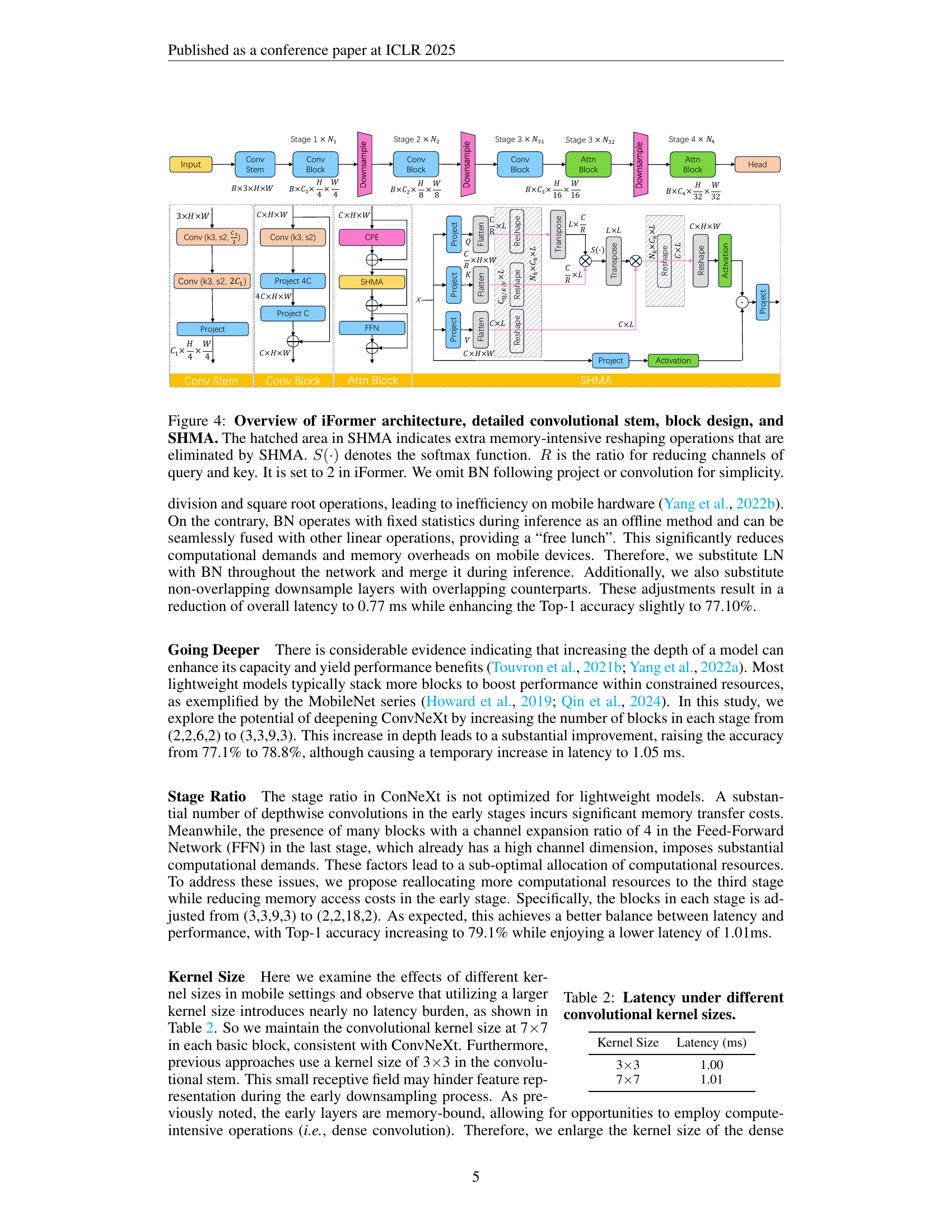
🔼 Figure 4 illustrates the architecture of the iFormer model, a hybrid convolutional and transformer network designed for mobile applications. It shows a hierarchical structure with four stages. Early stages use efficient convolutional blocks (derived from ConvNeXt) to extract local features quickly. Later stages incorporate a novel single-head modulation attention (SHMA) mechanism, depicted in detail. SHMA is designed to replace the computationally expensive multi-head self-attention, as shown by the hatched area representing operations removed in SHMA. The figure highlights the key components: a convolutional stem, convolutional blocks, attention blocks (using SHMA), and a final classification head. The use of a channel reduction ratio (R) in SHMA is also explained, set to 2 in this instance to improve efficiency. Batch Normalization (BN) is omitted from the diagram for simplicity.
read the caption
Figure 4: Overview of iFormer architecture, detailed convolutional stem, block design, and SHMA. The hatched area in SHMA indicates extra memory-intensive reshaping operations that are eliminated by SHMA. S(⋅)𝑆⋅S(\cdot)italic_S ( ⋅ ) denotes the softmax function. R𝑅Ritalic_R is the ratio for reducing channels of query and key. It is set to 2 in iFormer. We omit BN following project or convolution for simplicity.

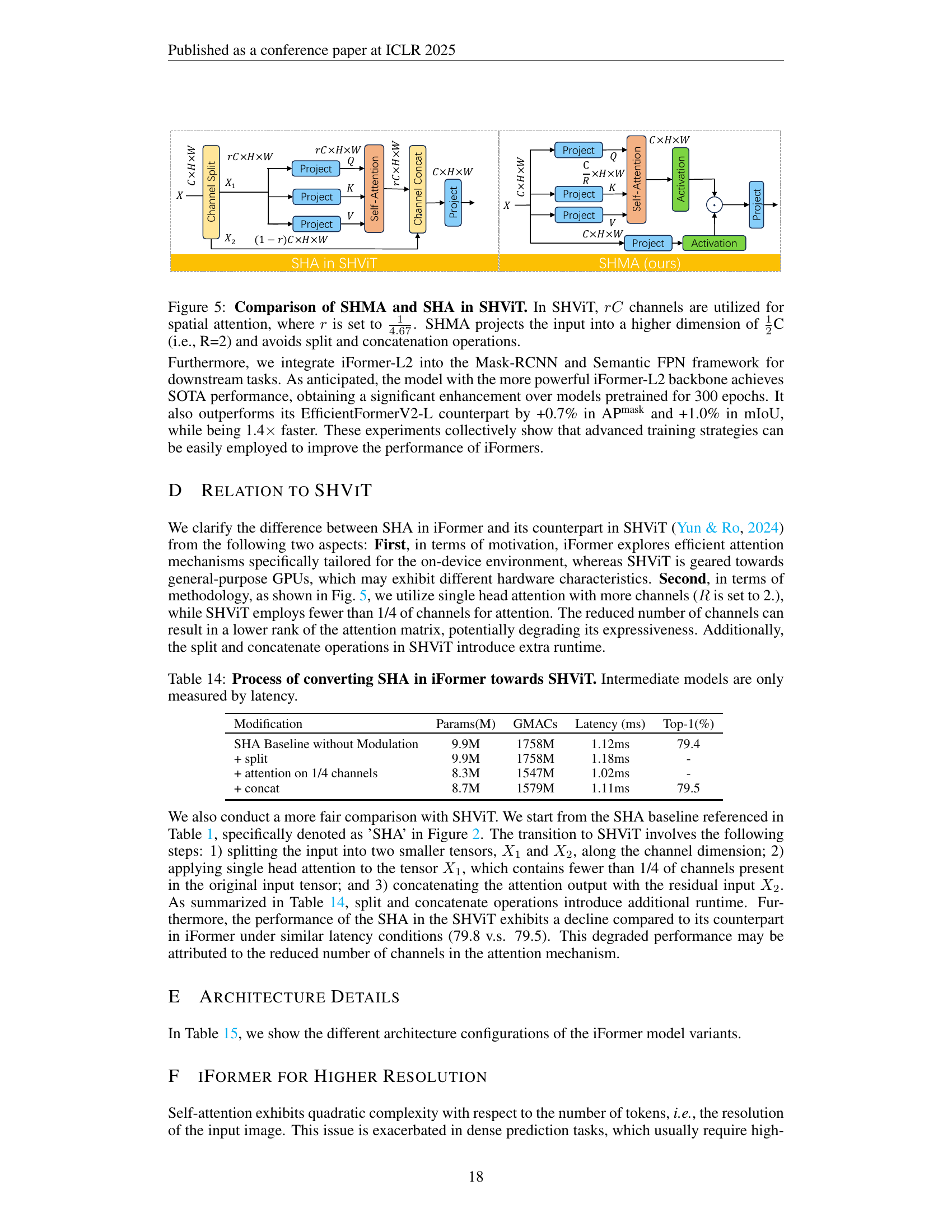
🔼 Figure 5 compares the single-head modulation attention (SHMA) proposed in the iFormer model with the single-head attention (SHA) used in the SHViT model. Both methods aim for efficient attention mechanisms in vision transformers, but they differ in their approach. SHViT uses only a fraction (1/4.67) of the input channels for spatial attention, requiring channel splitting and concatenation operations, which can be computationally expensive. In contrast, SHMA projects the input to a higher dimension (1.5 times the original) before the attention operation, avoiding these extra steps. This design choice enhances efficiency and reduces memory consumption.
read the caption
Figure 5: Comparison of SHMA and SHA in SHViT. In SHViT, rC𝑟𝐶rCitalic_r italic_C channels are utilized for spatial attention, where r𝑟ritalic_r is set to 14.6714.67\frac{1}{4.67}divide start_ARG 1 end_ARG start_ARG 4.67 end_ARG. SHMA projects the input into a higher dimension of 1212\frac{1}{2}divide start_ARG 1 end_ARG start_ARG 2 end_ARGC (i.e., R=2) and avoids split and concatenation operations.
More on tables
| Kernel Size | Latency (ms) |
| 33 | 1.00 |
| 77 | 1.01 |
🔼 This table presents the latency results measured on an iPhone 13 for different kernel sizes used in the convolutional layers of the iFormer model. It compares the efficiency of using different kernel sizes (3x3 and 7x7) in terms of inference speed, providing insights into the trade-off between computational cost and potential performance gains.
read the caption
Table 2: Latency under different convolutional kernel sizes.
| Model | Params (M) | GMACs | Latency (ms) | Reso. | Epochs | Top-1 (%) |
| MobileNetV2 1.0x (2018) | 3.4 | 0.30 | 0.73 | 224 | 500 | 72.0 |
| MobileNetV3-Large 0.75x (2019) | 4.0 | 0.16 | 0.67 | 224 | 600 | 73.3 |
| MNV4-Conv-S (2024) | 3.8 | 0.20 | 0.60 | 224 | 500 | 73.8 |
| iFormer-T | 2.9 | 0.53 | 0.60 | 224 | 300 | 74.1 |
| MobileNetV2 1.4x (2018) | 6.9 | 0.59 | 1.02 | 224 | 500 | 74.7 |
| MobileNetV3-Large 1.0x (2019) | 5.4 | 0.22 | 0.76 | 224 | 600 | 75.2 |
| SwiftFormer-XS (2023) | 3.5 | 0.60 | 0.95 | 224 | 300 | 75.7 |
| SBCFormer-XS (2024) | 5.6 | 0.70 | 0.79 | 224 | 300 | 75.8 |
| (2024) | 6.1 | 0.17 | 0.99 | 224 | 600 | 77.1 |
| MobileOne-S2 (2023b) | 7.8 | 1.30 | 0.92 | 224 | 300 | 77.4 |
| RepViT-M1.0 (2024) | 6.8 | 1.10 | 0.85 | 224 | 300 | 78.6 |
| iFormer-S | 6.5 | 1.09 | 0.85 | 224 | 300 | 78.8 |
| EfficientMod-xxs (2024) | 4.7 | 0.60 | 1.29 | 224 | 300 | 76.0 |
| SBCFormer-S (2024) | 8.5 | 0.90 | 1.02 | 224 | 300 | 77.7 |
| MobileOne-S3 (2023b) | 10.1 | 1.90 | 1.16 | 224 | 300 | 78.1 |
| SwiftFormer-S (2023) | 6.1 | 1.00 | 1.12 | 224 | 300 | 78.5 |
| (2024) | 8.9 | 0.27 | 1.24 | 224 | 600 | 79.1 |
| FastViT-T12 (2023a) | 6.8 | 1.40 | 1.12 | 256 | 300 | 79.1 |
| RepViT-M1.1 (2024) | 8.2 | 1.30 | 1.04 | 224 | 300 | 79.4 |
| MNV4-Conv-M (2024) | 9.2 | 1.00 | 1.08 | 256 | 500 | 79.9 |
| iFormer-M | 8.9 | 1.64 | 1.10 | 224 | 300 | 80.4 |
| Mobile-Former-294M (2022b) | 11.4 | 0.29 | 2.66 | 224 | 450 | 77.9 |
| MobileViT-S (2021) | 5.6 | 2.00 | 3.55 | 256 | 300 | 78.4 |
| MobileOne-S4 (2023b) | 14.8 | 2.98 | 1.74 | 224 | 300 | 79.4 |
| SBCFormer-B (2024) | 13.8 | 1.60 | 1.44 | 224 | 300 | 80.0 |
| (2024) | 12.3 | 0.40 | 1.49 | 224 | 600 | 80.4 |
| EfficientViT-B1-r288 (2023) | 9.1 | 0.86 | 3.87 | 288 | 450 | 80.4 |
| FastViT-SA12 (2023a) | 10.9 | 1.90 | 1.50 | 256 | 300 | 80.6 |
| MNV4-Hybrid-M (2024) | 10.5 | 1.20 | 1.75 | 256 | 500 | 80.7 |
| SwiftFormer-L1 (2023) | 12.1 | 1.60 | 1.60 | 224 | 300 | 80.9 |
| EfficientMod-s (2024) | 12.9 | 1.40 | 2.57 | 224 | 300 | 81.0 |
| RepViT-M1.5 (2024) | 14.0 | 2.30 | 1.54 | 224 | 300 | 81.2 |
| iFormer-L | 14.7 | 2.63 | 1.60 | 224 | 300 | 81.9 |
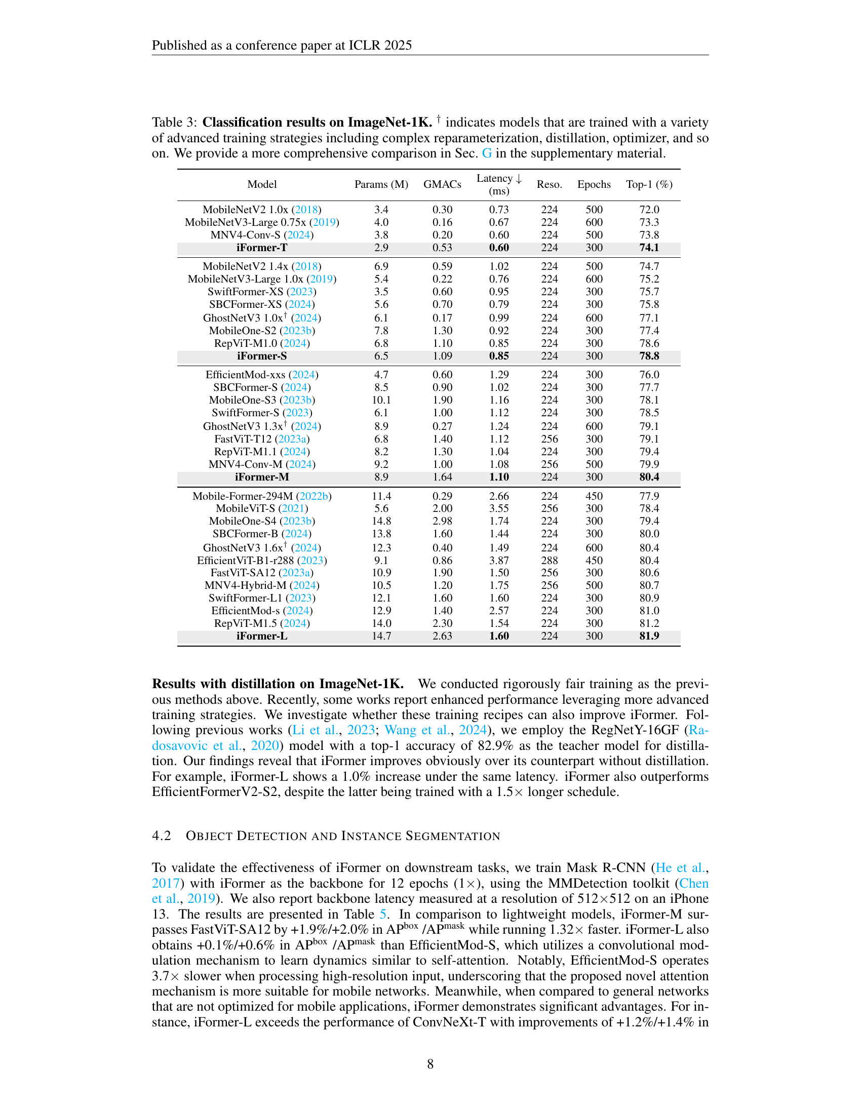
🔼 This table presents a comparison of various lightweight convolutional neural networks (CNNs) and vision transformers (ViTs) on the ImageNet-1K image classification benchmark. The table details several key metrics for each model, including the number of parameters (in millions), the number of Giga Multiply-Accumulates (GMACs, a measure of computational cost), the inference latency in milliseconds (ms) measured on an iPhone 13, input image resolution, number of training epochs, and the Top-1 accuracy (%). The † symbol indicates models trained using advanced techniques like reparameterization, distillation, or specialized optimizers, highlighting potential differences in training methodology that may affect performance comparison. More comprehensive results are available in the supplementary material (Section G).
read the caption
Table 3: Classification results on ImageNet-1K. † indicates models that are trained with a variety of advanced training strategies including complex reparameterization, distillation, optimizer, and so on. We provide a more comprehensive comparison in Sec. G in the supplementary material.
| Model | Latency (ms) | Reso. | Epochs | Top-1 (%) |
| EfficientFormerV2-S1 (2023) | 1.02 | 224 | 300 | 79.0 |
| EfficientFormerV2-S1 (2023) | 1.02 | 224 | 450 | 79.7 |
| MobileViGv2-S*(2024) | 1.24 | 224 | 300 | 79.8 |
| FastViT-T12* (2023a) | 1.12 | 256 | 300 | 80.3 |
| RepViT-M1.1* (2024) | 1.04 | 224 | 300 | 80.7 |
| iFormer-M | 1.10 | 224 | 300 | 81.1 |
| SHViT-S4 (2024) | 1.48 | 224 | 300 | 80.2 |
| EfficientFormerV2-S2 (2023) | 1.60 | 224 | 300 | 81.6 |
| MobileViGv2-M(2024) | 1.70 | 224 | 300 | 81.7 |
| FastViT-SA12* (2023a) | 1.50 | 256 | 300 | 81.9 |
| EfficientFormerV2-S2 (2023) | 1.60 | 224 | 450 | 82.0 |
| RepViT-M1.5* (2024) | 1.54 | 224 | 300 | 82.3 |
| iFormer-L | 1.60 | 224 | 300 | 82.7 |
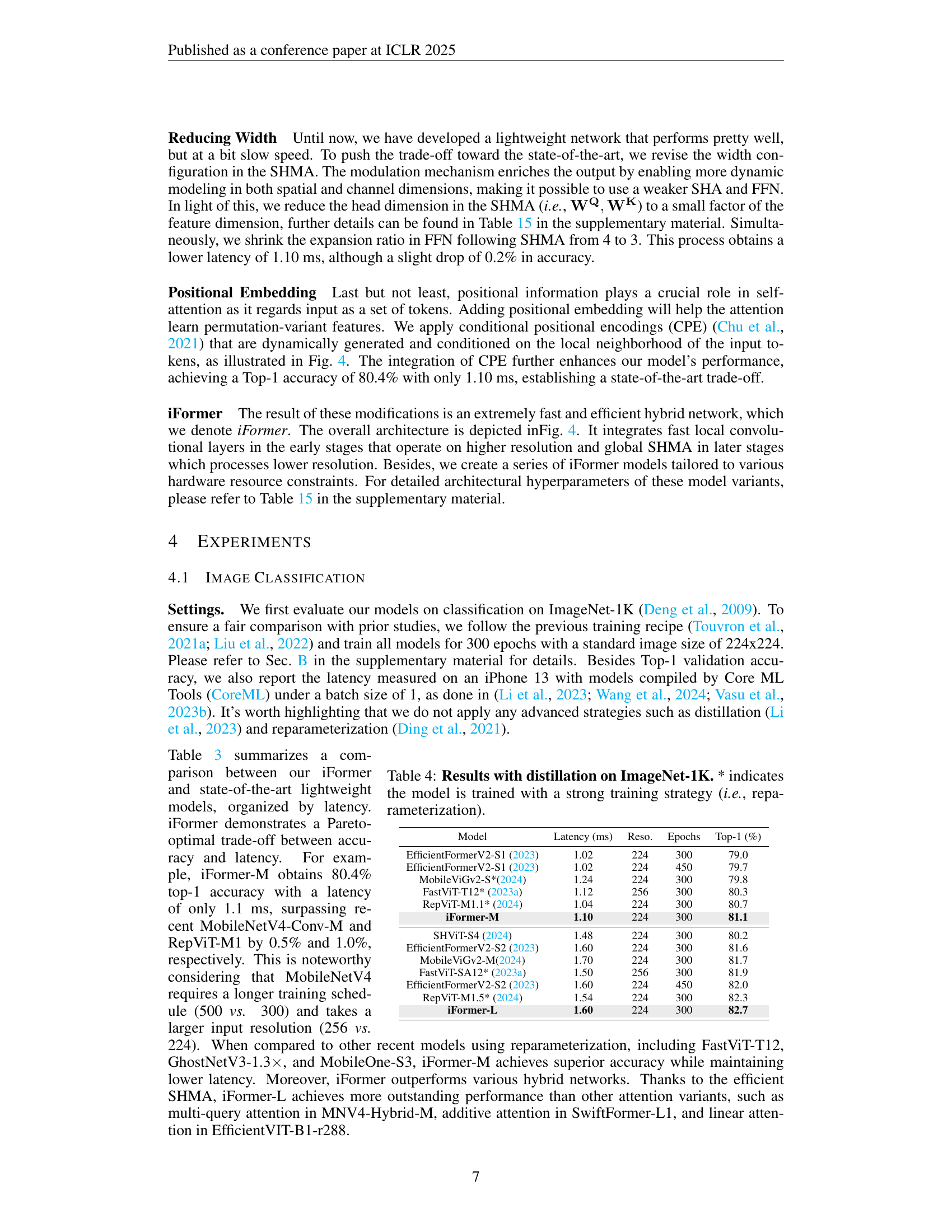
🔼 This table presents the ImageNet-1K classification results of several models trained with distillation. It compares the Top-1 accuracy and latency (measured on an iPhone 13) of different models, highlighting the impact of advanced training techniques like reparameterization on model performance. The asterisk (*) indicates models that used reparameterization during training.
read the caption
Table 4: Results with distillation on ImageNet-1K. * indicates the model is trained with a strong training strategy (i.e., reparameterization).
| Backbone | Param (M) | Latency (ms) | Object Detection | Instance Segmentation | Semantic | ||||
| AP | AP | AP | AP | AP | AP | mIoU | |||
| EfficientNet-B0 (2019) | 5.3 | 4.55 | 31.9 | 51.0 | 34.5 | 29.4 | 47.9 | 31.2 | - |
| ResNet18 (2016) | 11.7 | 2.85 | 34.0 | 54.0 | 36.7 | 31.2 | 51.0 | 32.7 | 32.9 |
| PoolFormer-S12 (2022) | 11.9 | 5.70 | 37.3 | 59.0 | 40.1 | 34.6 | 55.8 | 36.9 | 37.2 |
| EfficientFormer-L1 (2022b) | 12.3 | 3.50 | 37.9 | 60.3 | 41.0 | 35.4 | 57.3 | 37.3 | 38.9 |
| FastViT-SA12 (2023a) | 10.9 | 5.27 | 38.9 | 60.5 | 42.2 | 35.9 | 57.6 | 38.1 | 38.0 |
| RepViT-M1.1 (2024) | 8.2 | 3.18 | 39.8 | 61.9 | 43.5 | 37.2 | 58.8 | 40.1 | 40.6 |
| iFormer-M | 8.9 | 4.00 | 40.8 | 62.5 | 44.8 | 37.9 | 59.7 | 40.7 | 42.4 |
| ResNet50 (2016) | 25.5 | 7.20 | 38.0 | 58.6 | 41.4 | 34.4 | 55.1 | 36.7 | 36.7 |
| PoolFormer-S24 (2022) | 21.4 | 10.0 | 40.1 | 62.2 | 43.4 | 37.0 | 59.1 | 39.6 | 40.3 |
| ConvNeXt-T (Liu et al., 2022) | 29.0 | 13.6 | 41.0 | 62.1 | 45.3 | 37.7 | 59.3 | 40.4 | 41.4 |
| EfficientFormer-L3 (2022b) | 31.3 | 8.40 | 41.4 | 63.9 | 44.7 | 38.1 | 61.0 | 40.4 | 43.5 |
| RepViT-M1.5 (2024) | 14.0 | 5.00 | 41.6 | 63.2 | 45.3 | 38.6 | 60.5 | 41.5 | 43.6 |
| PVTv2-B1 (2022) | 14.0 | 27.00 | 41.8 | 64.3 | 45.9 | 38.8 | 61.2 | 41.6 | 42.5 |
| FastViT-SA24 (2023a) | 20.6 | 8.97 | 42.0 | 63.5 | 45.8 | 38.0 | 60.5 | 40.5 | 41.0 |
| EfficientMod-S (2024) | 32.6 | 24.30 | 42.1 | 63.6 | 45.9 | 38.5 | 60.8 | 41.2 | 43.5 |
| Swin-T (2021a) | 28.3 | Failed | 42.2 | 64.4 | 46.2 | 39.1 | 61.6 | 42.0 | 41.5 |
| iFormer-L | 14.7 | 6.60 | 42.2 | 64.2 | 46.0 | 39.1 | 61.4 | 41.9 | 44.5 |
🔼 This table presents a comparison of different model architectures on three computer vision tasks: object detection and instance segmentation on the MS COCO 2017 dataset, and semantic segmentation on the ADE20K dataset. The performance metrics include mean Average Precision (AP) for bounding boxes and masks, and mean Intersection over Union (mIoU) for semantic segmentation. Latency measurements, obtained using Core ML Tools on an iPhone 13 with 512x512 image crops, are also included to illustrate the computational efficiency of each model. ‘Failed’ indicates that the model’s inference time was too long to measure.
read the caption
Table 5: Object detection & instance segmentation results on MS COCO 2017 using Mask R-CNN. Semantic segmentation results on ADE20K using the Semantic FPN framework. We measure all backbone latencies with image crops of 512×\times×512 on iPhone 13 by Core ML Tools. Failed indicated that the model runs too long to report latency by the Core ML.
| SHMA Setting | Params (M) | GMACs | Latency (ms) | Top-1 Acc. (%) |
| SiLU + Post-BN | 8.9 | 1.60 | 1.10ms | Diverged |
| SiLU + Pre-LN | 8.9 | 1.64 | 1.17ms | 80.3 |
| Sigmoid + Post-BN | 8.9 | 1.60 | 1.10ms | 80.4 |
🔼 This table presents a comparison of different activation functions used within the Single-Head Modulation Attention (SHMA) mechanism of the iFormer model. It explores the impact of using Sigmoid, Sigmoid Linear Unit (SiLU), and their placement relative to Batch Normalization (BN) or Layer Normalization (LN) on the model’s performance. The results highlight the effect of these choices on accuracy and training stability, illustrating the trade-offs associated with different activation function choices.
read the caption
Table 6: Activation function comparison in SHMA. Post-BN indicates that BN is applied after projection. Pre-LN means that LN is implemented before the projection, as in standard MHA (Vaswani, 2017).
| Ratio Setting | Params (M) | GMACs | Latency (ms) | Top-1 Acc. (%) |
| Baseline | 9.4M | 1760M | 1.0ms | 79.4 |
| Replacing 22% Conv Blocks in Stage 3 as SHA | 9.1M | 1724M | 1.02ms | 79.5 |
| Replacing 22% Conv Blocks in Stage 3 as SHMA | 9.2M | 1739M | 1.04ms | 79.6 |
| Replacing 50% Conv Blocks in Stage 3 as SHA | 8.8M | 1689M | 1.04ms | 79.5 |
| Replacing 50% Conv Blocks in Stage 3 as SHMA | 8.9M | 1712M | 1.07ms | 79.8 |
| Replacing 78% Conv Blocks in Stage 3 as SHA | 8.3M | 1635M | 1.12ms | 79.3 |
| Replacing 78% Conv Blocks in Stage 3 as SHMA | 8.5M | 1685M | 1.17ms | 79.6 |
| Replacing 100% Conv Blocks in Stage 3 as SHA | 7.9M | 1599M | 1.17ms | 78.1 |
| Replacing 100% Conv Blocks in Stage 3 as SHMA | 8.3M | 1665M | 1.25ms | 79.0 |
| Replacing 100% Conv Blocks in Stage 3 as SHMA and 100% in Stage 4 | 10.0M | 1792M | 1.15ms | 80.4 |
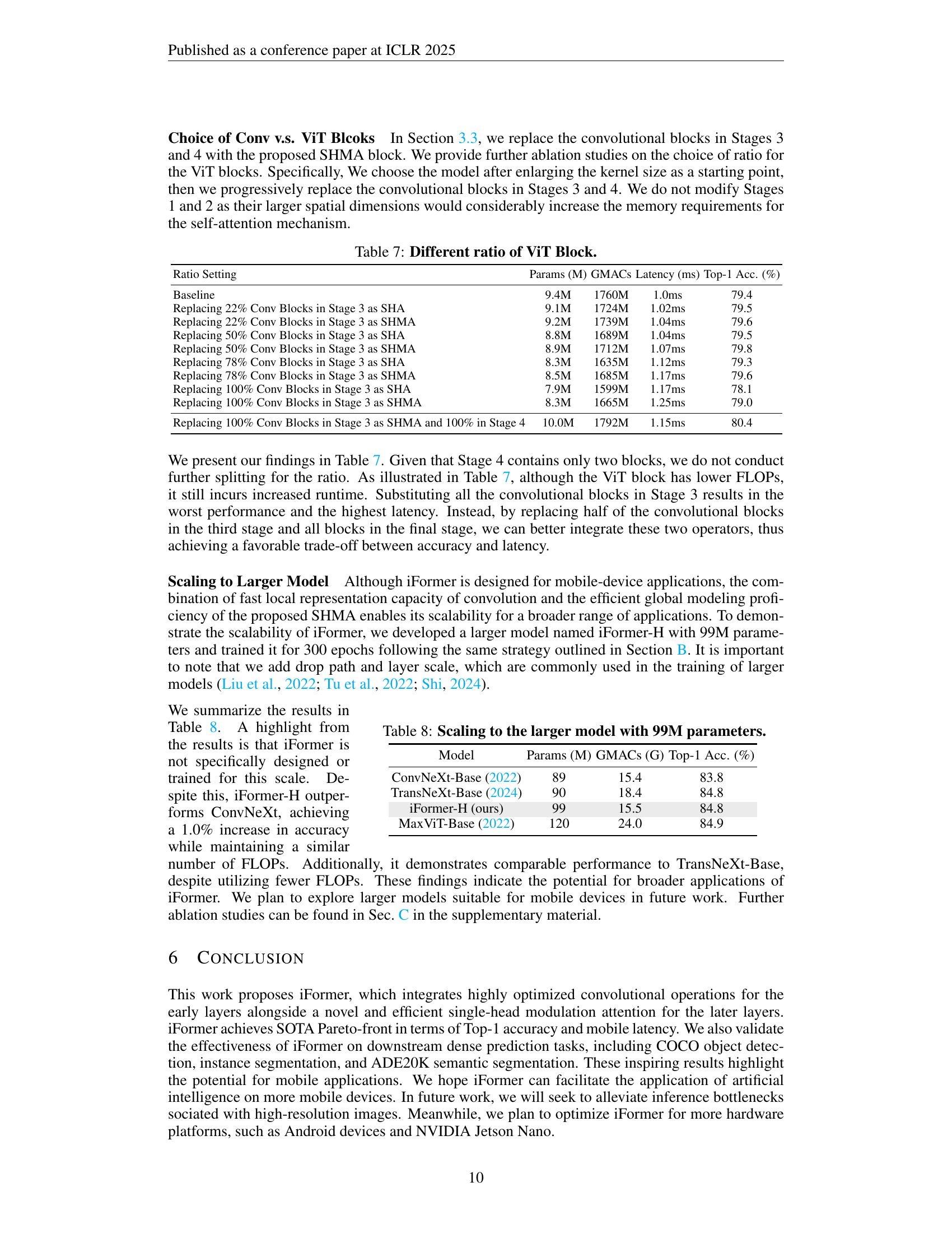
🔼 This table presents an ablation study on the impact of progressively replacing convolutional blocks with Vision Transformer (ViT) blocks in Stage 3 of the iFormer architecture. It shows the effect on model parameters (M), Giga multiply-accumulate operations (GMACS), latency (ms), and Top-1 accuracy (%) as the ratio of ViT blocks increases. This helps determine the optimal balance between latency and accuracy in the iFormer model.
read the caption
Table 7: Different ratio of ViT Block.
| Model | Params (M) | GMACs (G) | Top-1 Acc. (%) |
| ConvNeXt-Base (2022) | 89 | 15.4 | 83.8 |
| TransNeXt-Base (2024) | 90 | 18.4 | 84.8 |
| iFormer-H (ours) | 99 | 15.5 | 84.8 |
| MaxViT-Base (2022) | 120 | 24.0 | 84.9 |
🔼 This table presents the results of scaling up the iFormer model to 99 million parameters. It compares the performance (Top-1 accuracy) and computational cost (GMACs) of the larger iFormer-H model to other comparable models from the literature, demonstrating that iFormer scales effectively while maintaining competitive performance.
read the caption
Table 8: Scaling to the larger model with 99M parameters.
| training config | iFormer-T/S/M/L/H |
| resolution | 2242 |
| weight init | trunc. normal (0.2) |
| optimizer | AdamW |
| base learning rate | 4e-3 (T/S/M/L) 8e-3 |
| weight decay | 0.05 |
| optimizer momentum | |
| batch size | 4096 [T/S/M/L] 8192 [H] |
| training epochs | 300 |
| learning rate schedule | cosine decay |
| warmup epochs | 20 |
| warmup schedule | linear |
| layer-wise lr decay | None |
| randaugment | (9, 0.5) |
| mixup | 0.8 |
| cutmix | 1.0 |
| random erasing | 0.25 |
| label smoothing | 0.1 |
| stochastic depth | 0.0 [T/S/M] 0.1 [L] 0.6 [H] |
| layer scale | None [T/S/M/L] 1e-6 [H] |
| head init scale | None |
| gradient clip | None |
| exp. mov. avg. (EMA) | None |
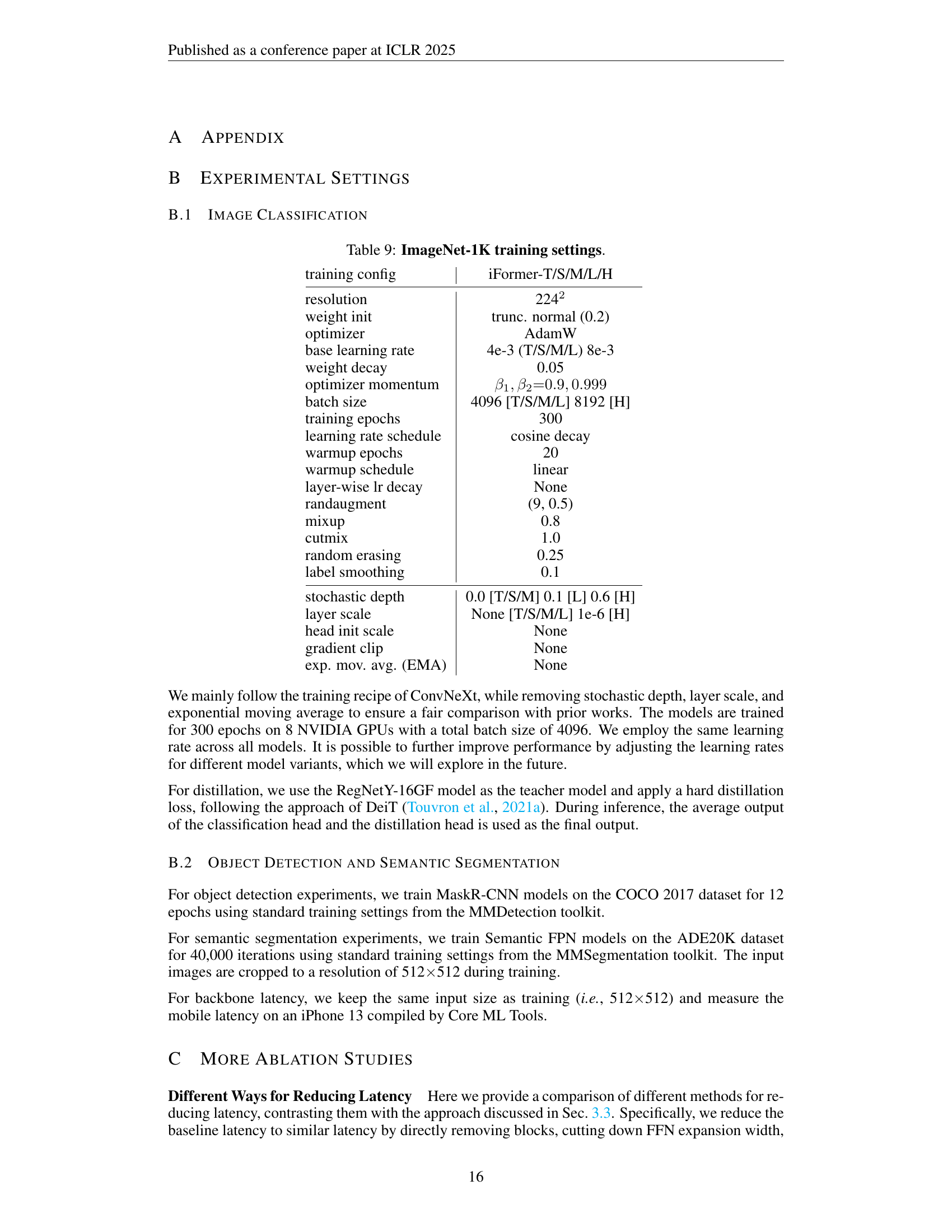
🔼 This table details the settings used for training image classification models on the ImageNet-1K dataset. It includes parameters such as image resolution, weight initialization method, optimizer, learning rate schedule (including warm-up), data augmentation techniques (RandAugment, Mixup, Cutmix, Random Erasing), label smoothing, and other training hyperparameters. These specifications are crucial for understanding and replicating the experimental results presented in the paper.
read the caption
Table 9: ImageNet-1K training settings.
| Reducing Setting | Params (M) | GMACs | Latency (ms) | Top-1 Acc. (%) |
| Baseline | 10.0 | 1.79 | 1.15 | 80.4 |
| Number of Blocks | 8.4 | 1.70 | 1.07 | 79.7 |
| FFN Width | 8.6 | 1.62 | 1.07 | 79.8 |
| Attn. Head and FFN Width | 8.9 | 1.64 | 1.10 | 80.2 |
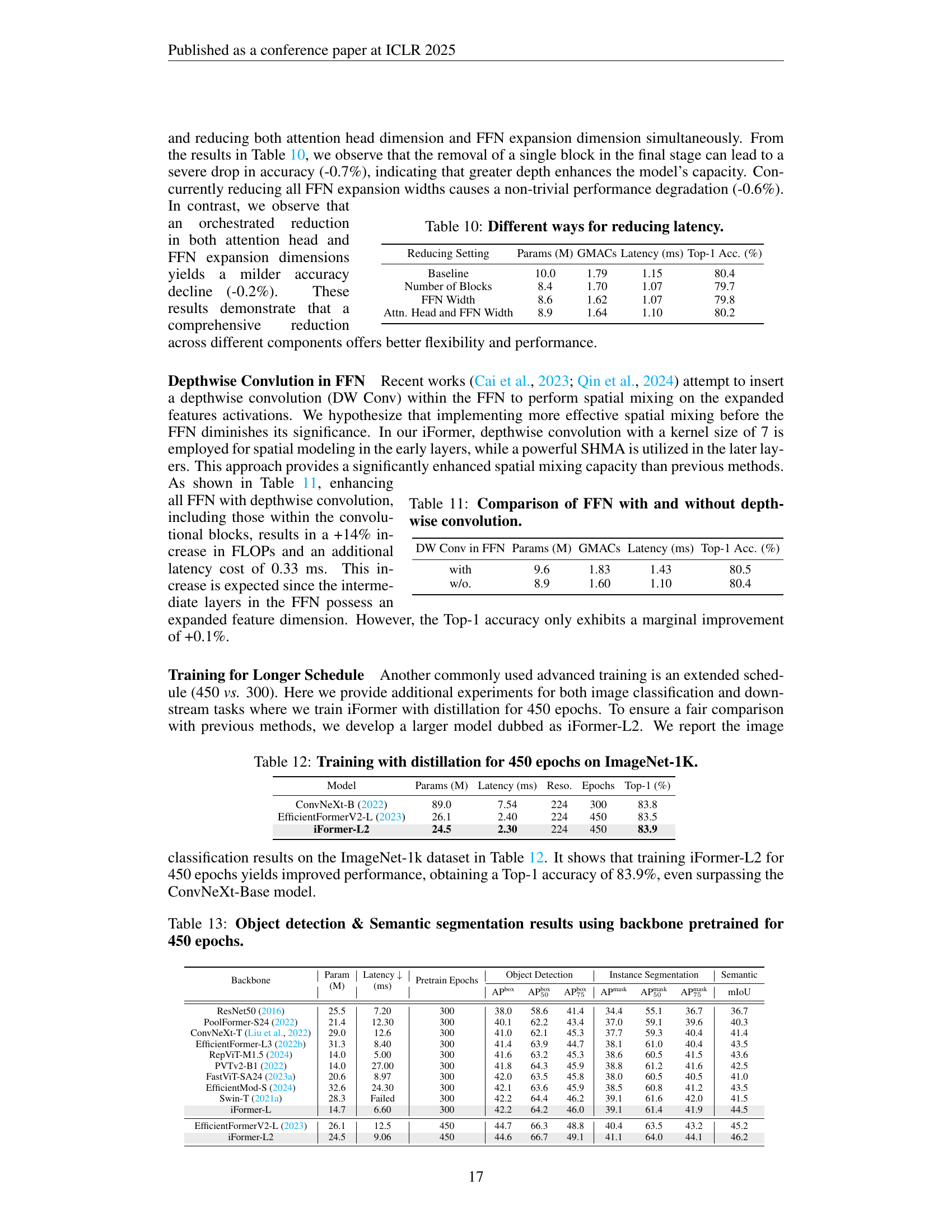
🔼 This table compares different methods for reducing latency in a lightweight neural network. It shows the impact on model parameters (in millions), GMACs (giga multiply-accumulate operations), latency (in milliseconds), and Top-1 accuracy (%) for several strategies: reducing the number of blocks, reducing the FFN (feed-forward network) width, and reducing both attention head dimension and FFN expansion width. The results highlight the trade-offs between latency reduction and accuracy.
read the caption
Table 10: Different ways for reducing latency.
| DW Conv in FFN | Params (M) | GMACs | Latency (ms) | Top-1 Acc. (%) |
| with | 9.6 | 1.83 | 1.43 | 80.5 |
| w/o. | 8.9 | 1.60 | 1.10 | 80.4 |
🔼 This table presents a comparison of the performance of Feed-Forward Networks (FFNs) with and without depthwise convolutions. It shows the impact of adding depthwise convolutions to the FFN on model parameters, GMACs (giga multiply-accumulate operations), latency (in milliseconds), and Top-1 accuracy on the ImageNet-1K dataset. This helps to assess the effectiveness of depthwise convolutions as a technique to improve performance within the FFN of a CNN model.
read the caption
Table 11: Comparison of FFN with and without depthwise convolution.
| Model | Params (M) | Latency (ms) | Reso. | Epochs | Top-1 (%) |
| ConvNeXt-B (2022) | 89.0 | 7.54 | 224 | 300 | 83.8 |
| EfficientFormerV2-L (2023) | 26.1 | 2.40 | 224 | 450 | 83.5 |
| iFormer-L2 | 24.5 | 2.30 | 224 | 450 | 83.9 |
🔼 This table presents the results of training various models, including the iFormer, on the ImageNet-1K dataset using distillation for 450 epochs. It compares the model’s performance in terms of parameters, latency (on an iPhone 13), resolution, and Top-1 accuracy. This extended training allows for a more thorough comparison of how different models perform under a longer training regime.
read the caption
Table 12: Training with distillation for 450 epochs on ImageNet-1K.
| Backbone | Param (M) | Latency (ms) | Pretrain Epochs | Object Detection | Instance Segmentation | Semantic | ||||
| AP | AP | AP | AP | AP | AP | mIoU | ||||
| ResNet50 (2016) | 25.5 | 7.20 | 300 | 38.0 | 58.6 | 41.4 | 34.4 | 55.1 | 36.7 | 36.7 |
| PoolFormer-S24 (2022) | 21.4 | 12.30 | 300 | 40.1 | 62.2 | 43.4 | 37.0 | 59.1 | 39.6 | 40.3 |
| ConvNeXt-T (Liu et al., 2022) | 29.0 | 12.6 | 300 | 41.0 | 62.1 | 45.3 | 37.7 | 59.3 | 40.4 | 41.4 |
| EfficientFormer-L3 (2022b) | 31.3 | 8.40 | 300 | 41.4 | 63.9 | 44.7 | 38.1 | 61.0 | 40.4 | 43.5 |
| RepViT-M1.5 (2024) | 14.0 | 5.00 | 300 | 41.6 | 63.2 | 45.3 | 38.6 | 60.5 | 41.5 | 43.6 |
| PVTv2-B1 (2022) | 14.0 | 27.00 | 300 | 41.8 | 64.3 | 45.9 | 38.8 | 61.2 | 41.6 | 42.5 |
| FastViT-SA24 (2023a) | 20.6 | 8.97 | 300 | 42.0 | 63.5 | 45.8 | 38.0 | 60.5 | 40.5 | 41.0 |
| EfficientMod-S (2024) | 32.6 | 24.30 | 300 | 42.1 | 63.6 | 45.9 | 38.5 | 60.8 | 41.2 | 43.5 |
| Swin-T (2021a) | 28.3 | Failed | 300 | 42.2 | 64.4 | 46.2 | 39.1 | 61.6 | 42.0 | 41.5 |
| iFormer-L | 14.7 | 6.60 | 300 | 42.2 | 64.2 | 46.0 | 39.1 | 61.4 | 41.9 | 44.5 |
| EfficientFormerV2-L (2023) | 26.1 | 12.5 | 450 | 44.7 | 66.3 | 48.8 | 40.4 | 63.5 | 43.2 | 45.2 |
| iFormer-L2 | 24.5 | 9.06 | 450 | 44.6 | 66.7 | 49.1 | 41.1 | 64.0 | 44.1 | 46.2 |
🔼 This table presents the results of object detection and semantic segmentation experiments. The models used had backbones pretrained for 450 epochs, and the results are compared across various backbone architectures. Metrics shown include bounding box average precision (APbox), mask average precision (Apmask), and mean Intersection over Union (mIoU) for semantic segmentation. This allows for assessment of the impact of the longer pretraining on downstream task performance.
read the caption
Table 13: Object detection & Semantic segmentation results using backbone pretrained for 450 epochs.
| Modification | Params(M) | GMACs | Latency (ms) | Top-1(%) |
| SHA Baseline without Modulation | 9.9M | 1758M | 1.12ms | 79.4 |
| + split | 9.9M | 1758M | 1.18ms | - |
| + attention on 1/4 channels | 8.3M | 1547M | 1.02ms | - |
| + concat | 8.7M | 1579M | 1.11ms | 79.5 |
🔼 This table details the step-by-step process of modifying the single-head attention (SHA) mechanism from the iFormer model to match the SHA in the SHViT model. It shows how modifications, such as adding splitting and concatenation operations, and reducing the number of channels used in attention, affect the model’s latency and top-1 accuracy. Intermediate models’ accuracy is not reported because the changes were made only for testing latency.
read the caption
Table 14: Process of converting SHA in iFormer towards SHViT. Intermediate models are only measured by latency.
| iFormer-T | iFormer-S | iFormer-M | iFormer-L | |||
| Stem | 5656 (4) | 1 | 1 | 1 | 1 | ||
| 1 | 1 | 1 | 1 | ||||
| Stage 1 | 5656 (4) | 2 | 2 | 2 | 2 | ||
| Stage 2 | 2828 (8) | 1 | 1 | 1 | 1 | ||
| 2 | 2 | 2 | 2 | ||||
| Stage 3 | 1414 (16) | 1 | 1 | 1 | 1 | ||
| 6 | 9 | 9 | 8 | ||||
| 3 | 3 | 4 | 8 | ||||
| 1 | 1 | 1 | 1 | ||||
| Stage 4 | 77 (32) | 1 | 1 | 1 | 1 | ||
| 2 | 2 | 2 | 2 | ||||
| Params (M) | 2.9 | 6.5 | 8.9 | 14.7 | |||
| GMacs | 0.53 | 1.09 | 1.64 | 2.63 | |||
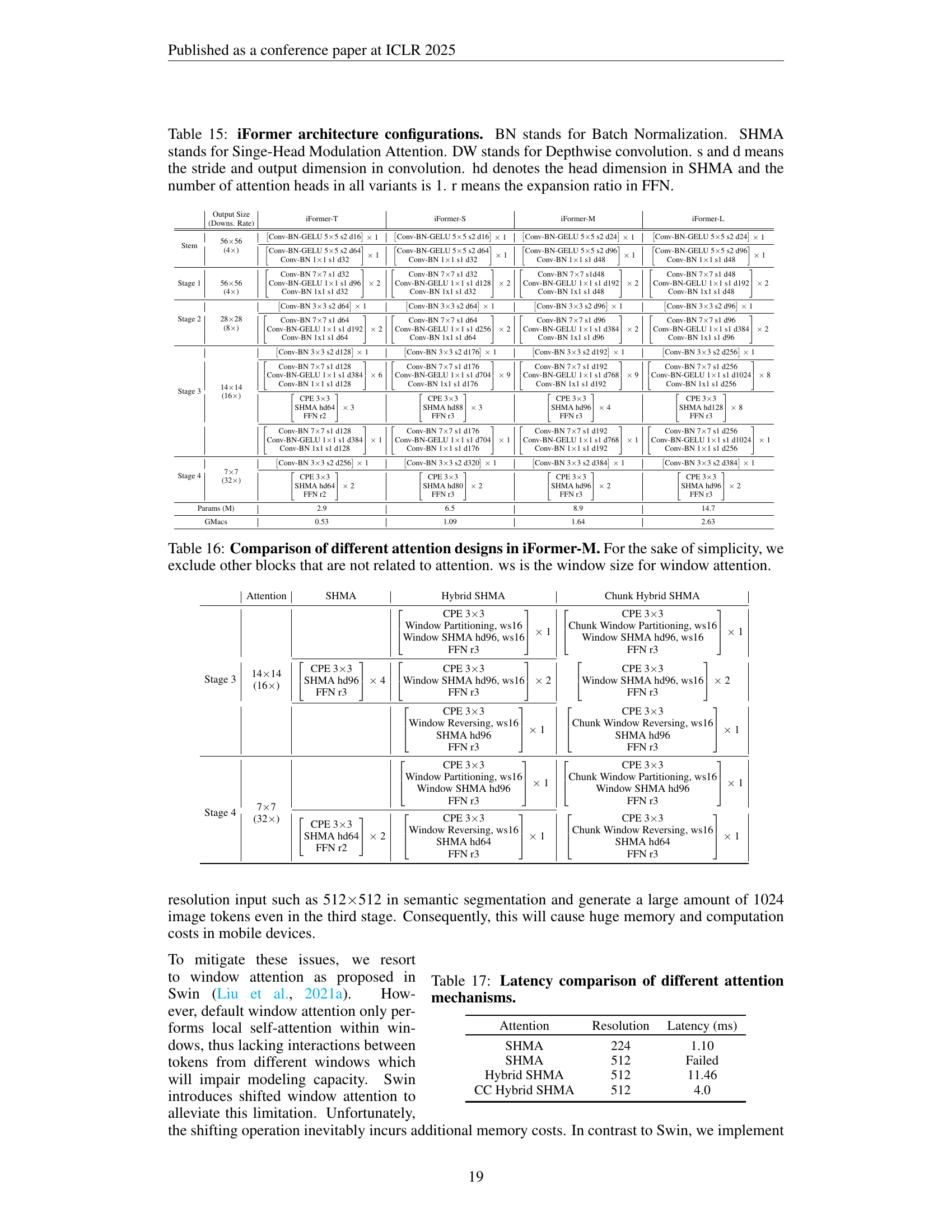
🔼 Table 15 provides detailed architectural configurations for different variants of the iFormer model (iFormer-T, iFormer-S, iFormer-M, iFormer-L). It outlines the specifications for each stage of the network, including the convolutional stem and blocks. Key parameters such as the number of convolutional blocks, kernel size (Conv), stride (s), output dimension (d), Batch Normalization (BN) usage, and GELU activation function are explicitly listed for each stage. The table also details the Single-Head Modulation Attention (SHMA) configurations for each stage, specifically noting the head dimension (hd) and the expansion ratio (r) in the Feed-Forward Network (FFN). The consistent use of a single attention head (1) across all variants is highlighted.
read the caption
Table 15: iFormer architecture configurations. BN stands for Batch Normalization. SHMA stands for Singe-Head Modulation Attention. DW stands for Depthwise convolution. s and d means the stride and output dimension in convolution. hd denotes the head dimension in SHMA and the number of attention heads in all variants is 1. r means the expansion ratio in FFN.
| Output Size |
| (Downs. Rate) |
🔼 This table compares different attention mechanisms used in the iFormer-M model, focusing on the design choices within the attention blocks (Stage 3 and 4) and their impact on performance. It contrasts the basic single-head modulation attention (SHMA) with several variations that incorporate window partitioning, window reversing, and combinations thereof. The table helps to understand the tradeoffs between different architectural options for balancing efficiency and accuracy. The ‘ws’ parameter indicates the window size used in window-based attention methods. Other parts of the network, not directly related to attention, are excluded for simplicity.
read the caption
Table 16: Comparison of different attention designs in iFormer-M. For the sake of simplicity, we exclude other blocks that are not related to attention. ws is the window size for window attention.
| Attention | SHMA | Hybrid SHMA | Chunk Hybrid SHMA | |
| Stage 3 | 1414 (16) | 1 | 1 | |
| 4 | 2 | 2 | ||
| 1 | 1 | |||
| Stage 4 | 77 (32) | 1 | 1 | |
| 2 | 1 | 1 |
🔼 This table compares the latency of different attention mechanisms on an iPhone 13. The latency is measured for two different input resolutions (224x224 and 512x512). The table shows that the standard single-head modulation attention (SHMA) is faster for 224x224 resolution but fails to produce results within a reasonable timeframe for 512x512 resolution. In contrast, the Hybrid SHMA and Chunk Hybrid SHMA methods are able to handle the higher resolution, with Chunk Hybrid SHMA demonstrating significantly better performance. This highlights the effectiveness of the proposed chunking strategy in addressing the computational challenges of high-resolution inputs.
read the caption
Table 17: Latency comparison of different attention mechanisms.
| Attention | Resolution | Latency (ms) |
| SHMA | 224 | 1.10 |
| SHMA | 512 | Failed |
| Hybrid SHMA | 512 | 11.46 |
| CC Hybrid SHMA | 512 | 4.0 |
🔼 This table presents a comprehensive comparison of iFormer’s performance against other lightweight models on the ImageNet-1K dataset. Metrics include the number of model parameters (in millions), the number of multiply-accumulate operations (GMACS), inference latency (in milliseconds) measured on an iPhone 13 using Core ML, input image resolution, number of training epochs, and finally the Top-1 accuracy achieved. Note that ‘Failed’ indicates models where latency measurement was not possible due to excessively long runtimes, usually attributed to memory limitations on the device.
read the caption
Table 18: Comprehensive comparison between iFormer and the previously proposed models on ImageNet-1K. Failed indicated that the model runs too long to report latency by the Core ML, often caused by excessive memory access.
Full paper#