TL;DR#
Diffusion Bridge Models (DBMs) are powerful for image-to-image tasks, but their slow inference hinders practical use. Existing acceleration methods are limited, often applying only to specific DBM types or falling short in achieving single-step generation. This creates a need for a universal and efficient acceleration technique.
This paper introduces Inverse Bridge Matching Distillation (IBMD), a new method that addresses these limitations. IBMD offers a universal approach, working with both conditional and unconditional DBMs. It allows for distillation into single-step generators and doesn’t require target domain data. Evaluations across numerous tasks show that IBMD significantly speeds up DBMs inference (4x to 100x) and can even improve generation quality compared to the original models.
Key Takeaways#
Why does it matter?#
This paper is crucial because it tackles the slow inference issue in Diffusion Bridge Models (DBMs), a significant hurdle limiting their wider adoption. By introducing a novel distillation technique, it offers a universal solution for accelerating both conditional and unconditional DBMs, paving the way for more efficient applications in various image-to-image translation tasks. The proposed method’s data-free distillation aspect and its demonstration of improved generation quality further enhance its significance for researchers seeking efficient and high-performing DBMs.
Visual Insights#

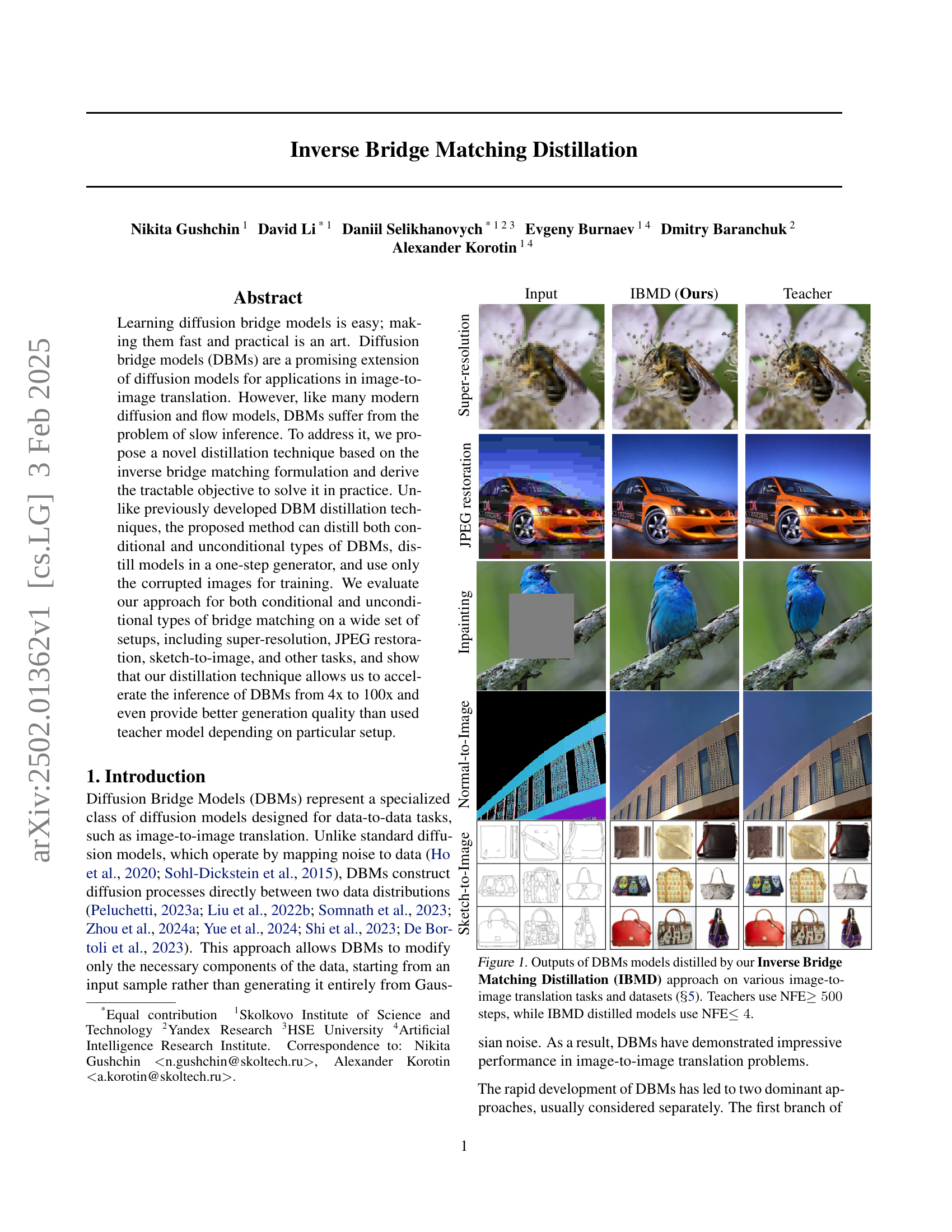
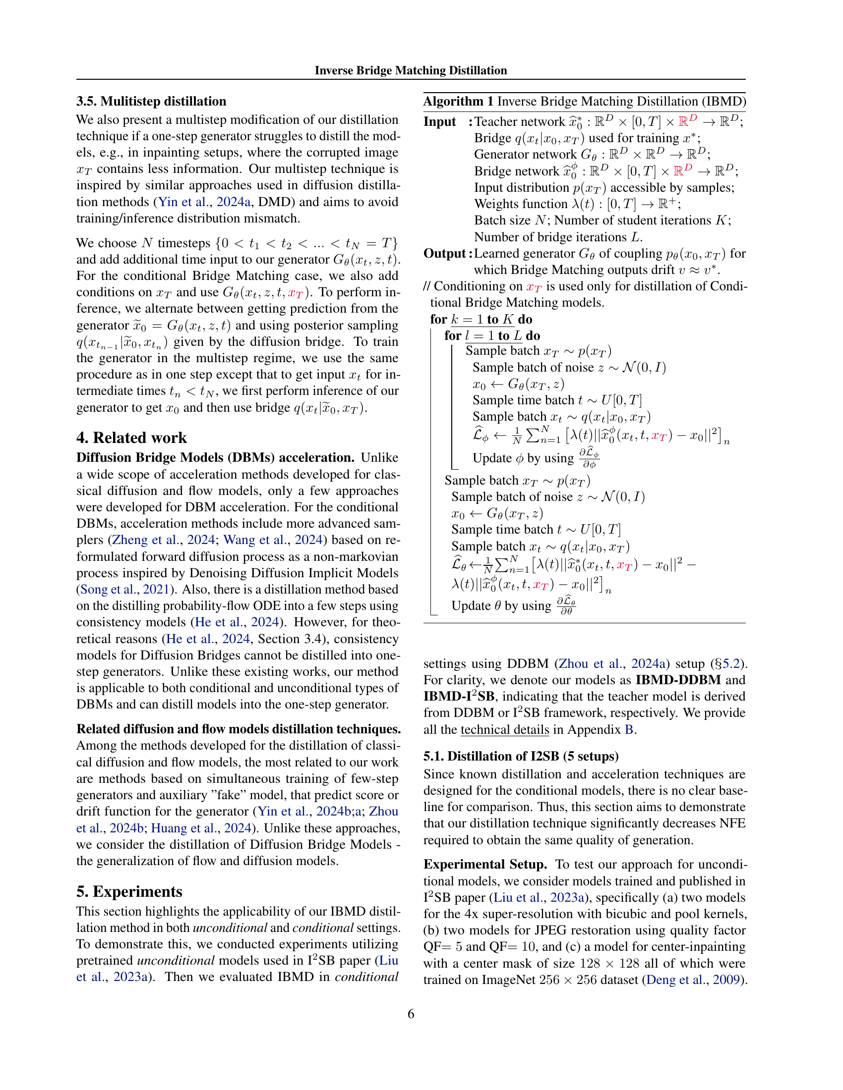
🔼 This figure showcases the results of the Inverse Bridge Matching Distillation (IBMD) technique on several image-to-image translation tasks. It presents visual comparisons between the outputs of original diffusion bridge models (DBMs), which required 500 or more steps for inference, and the outputs of DBMs distilled using the IBMD method. The distilled models achieve comparable or even better image quality using only 4 or fewer steps, demonstrating significant improvements in efficiency. The tasks include super-resolution, inpainting, JPEG restoration, and sketch-to-image translation.
read the caption
Figure 1: Outputs of DBMs models distilled by our Inverse Bridge Matching Distillation (IBMD) approach on various image-to-image translation tasks and datasets (\wasyparagraph5). Teachers use NFE≥500absent500\geq 500≥ 500 steps, while IBMD distilled models use NFE≤4absent4\leq 4≤ 4.
| Input | IBMD (Ours) | Teacher | |
| Super-resolution |  |  |  |
| JPEG restoration |  |  |  |
| Inpainting |  |  |  |
| Normal-to-Image |  |  |  |
| Sketch-to-Image |  |  |  |
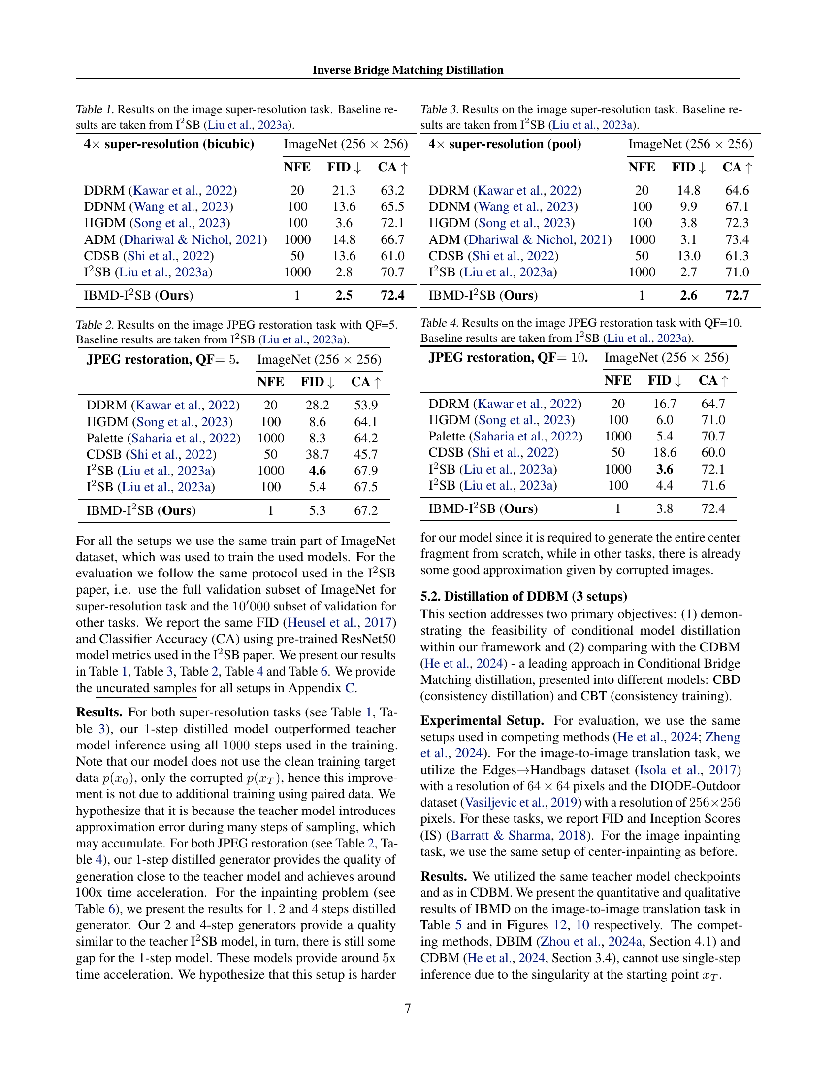
🔼 This table presents a comparison of different models on the image super-resolution task, specifically focusing on the Fréchet Inception Distance (FID) and Classifier Accuracy (CA) metrics. It compares the performance of several state-of-the-art diffusion models, including DDRM, DDNM, IGDM, ADM, and CDSB, along with the I2SB model which serves as a baseline. The main focus is to show that the proposed IBMD method, with only 1 network forward evaluation (NFE), outperforms the existing models or performs comparably while requiring significantly fewer forward passes. Lower FID scores and higher CA scores indicate better performance.
read the caption
Table 1: Results on the image super-resolution task. Baseline results are taken from I2SB (Liu et al., 2023a).
In-depth insights#
DBM Distillation#
Diffusion Bridge Models (DBMs) are powerful for image-to-image translation, but their multistep inference is slow. DBM distillation aims to address this by training a smaller, faster student model to mimic a larger, slower teacher DBM. This is crucial for practical applications where speed is a significant factor. Effective distillation techniques need to capture the complex data transformations learned by the teacher DBM while maintaining high-quality output. Key challenges include: (1) handling both conditional and unconditional DBMs, (2) achieving a good balance between speed and accuracy in the student model, and (3) designing a loss function that effectively guides the student model’s training. The success of DBM distillation directly impacts the real-world usability of DBMs, opening the door for wider adoption in areas like image editing, super-resolution, and style transfer, if it can achieve sufficient speed improvements without compromising quality. Therefore, research efforts in this area are important for realizing the full potential of DBMs.
IBMD Approach#
The Inverse Bridge Matching Distillation (IBMD) approach presents a novel distillation technique for accelerating Diffusion Bridge Models (DBMs). Its key innovation lies in tackling the inverse bridge matching problem, offering a universal solution applicable to both conditional and unconditional DBMs. Unlike previous methods, IBMD effectively distills models into one-step generators, significantly speeding up inference. The method’s strength is highlighted by its data-free distillation, requiring only corrupted images for training and its ability to improve the quality of generation compared to the teacher model in various scenarios. While the approach demonstrates impressive speedups and improved quality, the computational cost of the distillation process itself remains a potential area for future optimization.
Inverse Problem#
The core of the inverse problem in this research lies in reversing the diffusion process to learn a generator that can effectively create data samples. Instead of directly training the generator to match the target data distribution, the authors cleverly formulate the problem as an optimization task to find the underlying distribution from which the observed corrupted images originate. This inverse approach avoids explicit reliance on clean data during the training phase, thereby significantly simplifying the training process and making it more practical. By framing it as an optimization problem, the authors then introduce a tractable solution, offering a novel and efficient distillation technique. This approach is particularly impactful for diffusion bridge models because it addresses the inherent challenge of slow inference often associated with such models. The inverse problem’s solution, therefore, allows for faster and potentially higher-quality generation of the desired outputs, presenting a significant advancement in diffusion model applications.
Experimental Setup#
A robust “Experimental Setup” section in a research paper is crucial for reproducibility and validation. It should detail the specific datasets used, including their size, preprocessing steps (e.g., normalization, augmentation), and any relevant statistics. The description of the models employed must include their architectures, hyperparameters, and training procedures. Clearly specifying the training process is vital, including metrics used, optimization algorithms, and the hardware used for training and inference. The evaluation metrics chosen must be explicitly defined and justified in relation to the research question. Finally, a detailed description of the experimental protocols, including the number of runs, any random seeds, and the handling of randomness, guarantees that others can replicate the study, verifying the findings and promoting the advancement of the field.
Future Works#
Future research directions stemming from this Inverse Bridge Matching Distillation (IBMD) paper could explore several promising avenues. Extending IBMD to other diffusion models beyond DBMs is a key area. The current work focuses on DBMs, but the underlying principles might generalize to other architectures. Investigating the applicability of IBMD to different data modalities such as audio, time-series, and 3D data would broaden its impact. Furthermore, a deeper theoretical understanding of why IBMD improves generation quality in some cases compared to the teacher model is needed. This might involve analyzing the relationship between the inverse bridge matching problem and the expressiveness of the distilled model. Improving efficiency and scalability of the IBMD algorithm is crucial for wider adoption. The current method can be computationally expensive, so exploring optimized training strategies or alternative formulations are important. Finally, exploring the potential for combining IBMD with other acceleration techniques like improved samplers or score-based methods could lead to even faster and higher-quality diffusion model inference.
More visual insights#
More on figures
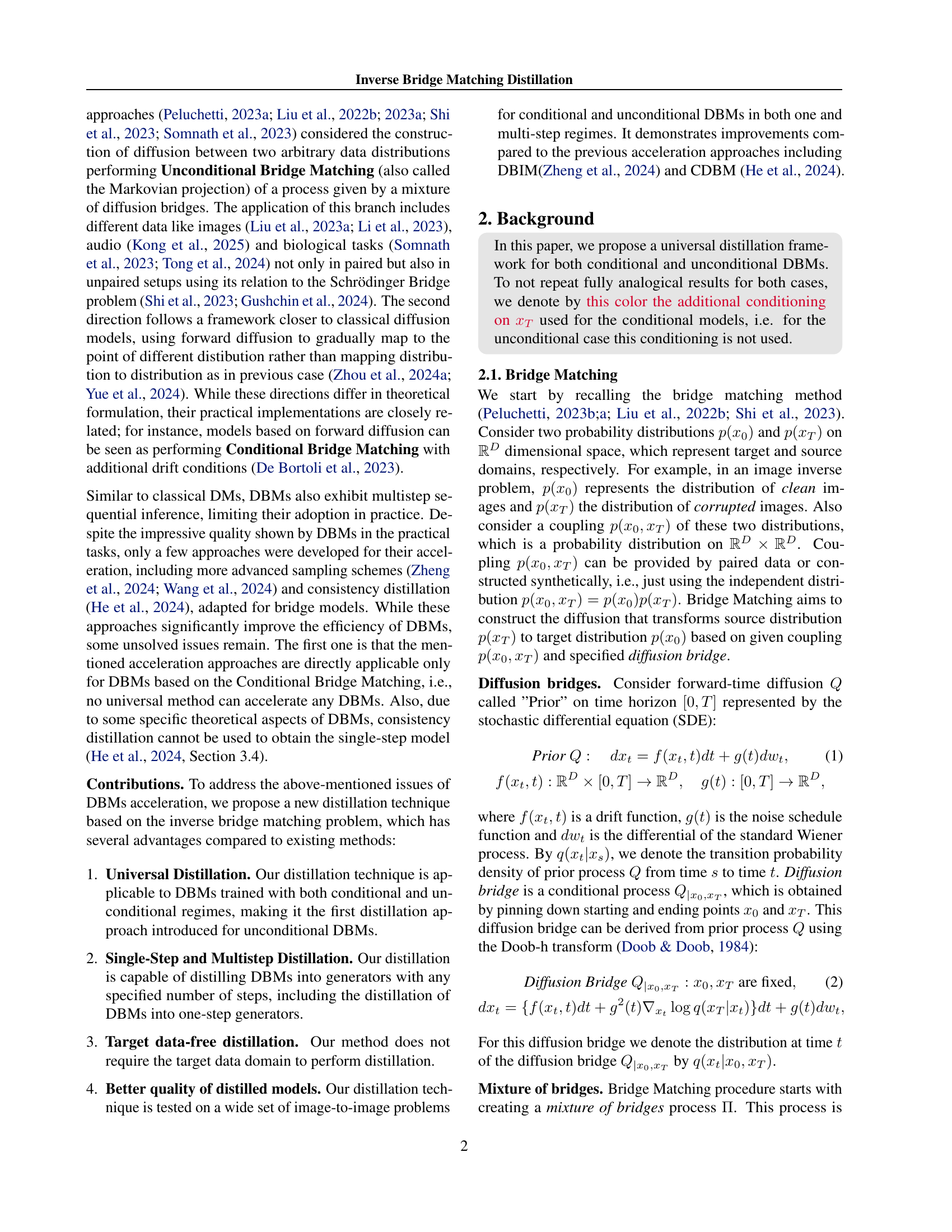
🔼 Figure 2 illustrates the process of Bridge Matching, a method for constructing a diffusion process between two data distributions. It shows how an intermediate sample is drawn from a diffusion bridge at a random time point, and the model learns to reconstruct the starting point from this intermediate sample. The figure also illustrates the conditional version, where an additional input is used to improve reconstruction.
read the caption
Figure 2: Overview of (Conditional) Bridge Matching with x^0subscript^𝑥0\widehat{x}_{0}over^ start_ARG italic_x end_ARG start_POSTSUBSCRIPT 0 end_POSTSUBSCRIPT reparameterization. The process begins by sampling a pair (x0,xT)subscript𝑥0subscript𝑥𝑇(x_{0},x_{T})( italic_x start_POSTSUBSCRIPT 0 end_POSTSUBSCRIPT , italic_x start_POSTSUBSCRIPT italic_T end_POSTSUBSCRIPT ) from the data coupling p(x0,xT)𝑝subscript𝑥0subscript𝑥𝑇p(x_{0},x_{T})italic_p ( italic_x start_POSTSUBSCRIPT 0 end_POSTSUBSCRIPT , italic_x start_POSTSUBSCRIPT italic_T end_POSTSUBSCRIPT ). An intermediate sample xtsubscript𝑥𝑡x_{t}italic_x start_POSTSUBSCRIPT italic_t end_POSTSUBSCRIPT is then drawn from the diffusion bridge q(xt|x0,xT)𝑞conditionalsubscript𝑥𝑡subscript𝑥0subscript𝑥𝑇q(x_{t}|x_{0},x_{T})italic_q ( italic_x start_POSTSUBSCRIPT italic_t end_POSTSUBSCRIPT | italic_x start_POSTSUBSCRIPT 0 end_POSTSUBSCRIPT , italic_x start_POSTSUBSCRIPT italic_T end_POSTSUBSCRIPT ) at a random time t∼U[0,T]similar-to𝑡𝑈0𝑇t\sim U[0,T]italic_t ∼ italic_U [ 0 , italic_T ]. The model x^0subscript^𝑥0\widehat{x}_{0}over^ start_ARG italic_x end_ARG start_POSTSUBSCRIPT 0 end_POSTSUBSCRIPT is trained with an MSE loss to reconstruct x0subscript𝑥0x_{0}italic_x start_POSTSUBSCRIPT 0 end_POSTSUBSCRIPT from xtsubscript𝑥𝑡x_{t}italic_x start_POSTSUBSCRIPT italic_t end_POSTSUBSCRIPT. In the conditional setting (dashed red path), x^0subscript^𝑥0\widehat{x}_{0}over^ start_ARG italic_x end_ARG start_POSTSUBSCRIPT 0 end_POSTSUBSCRIPT is also conditioned on xTsubscript𝑥𝑇x_{T}italic_x start_POSTSUBSCRIPT italic_T end_POSTSUBSCRIPT as an additional input, leveraging information about the terminal state to improve reconstruction.

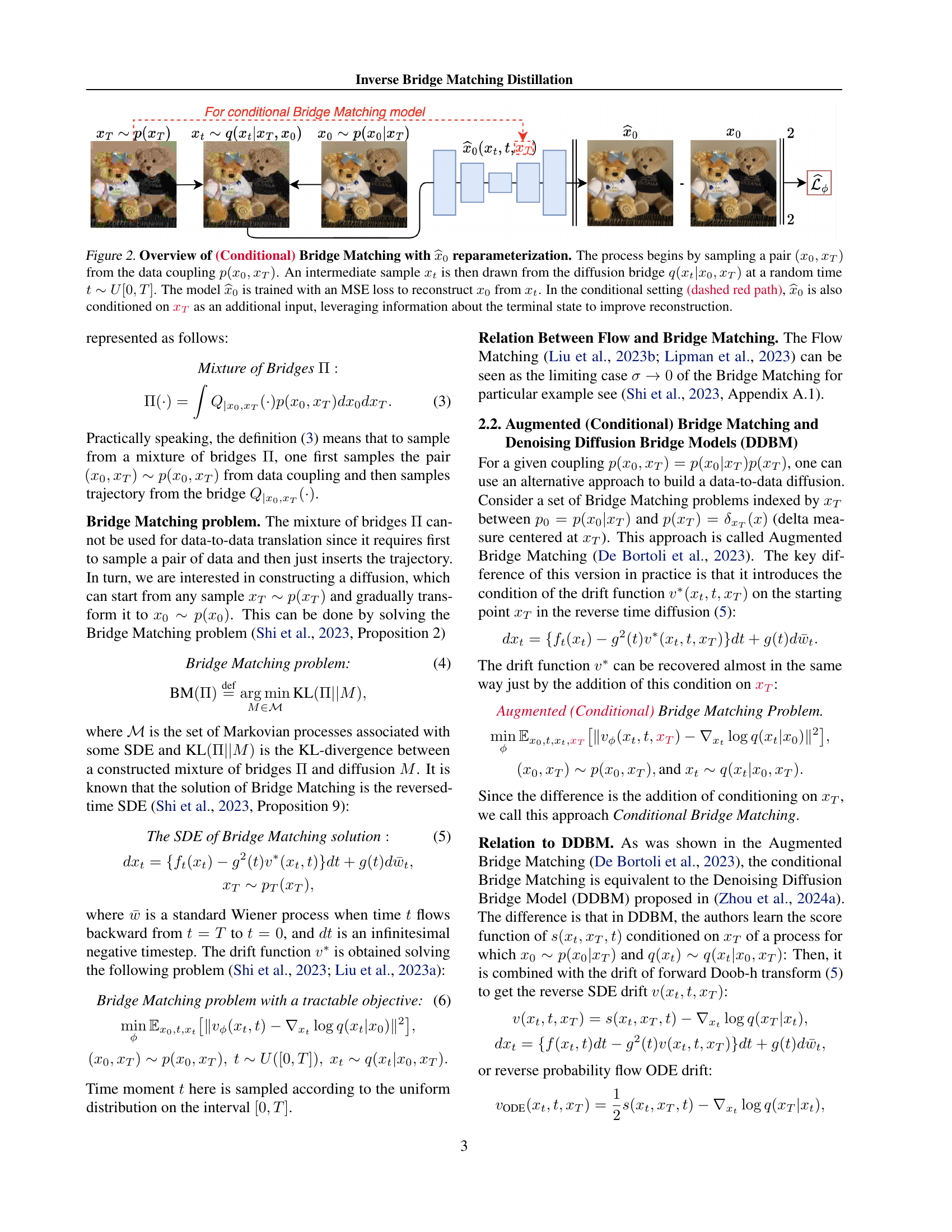
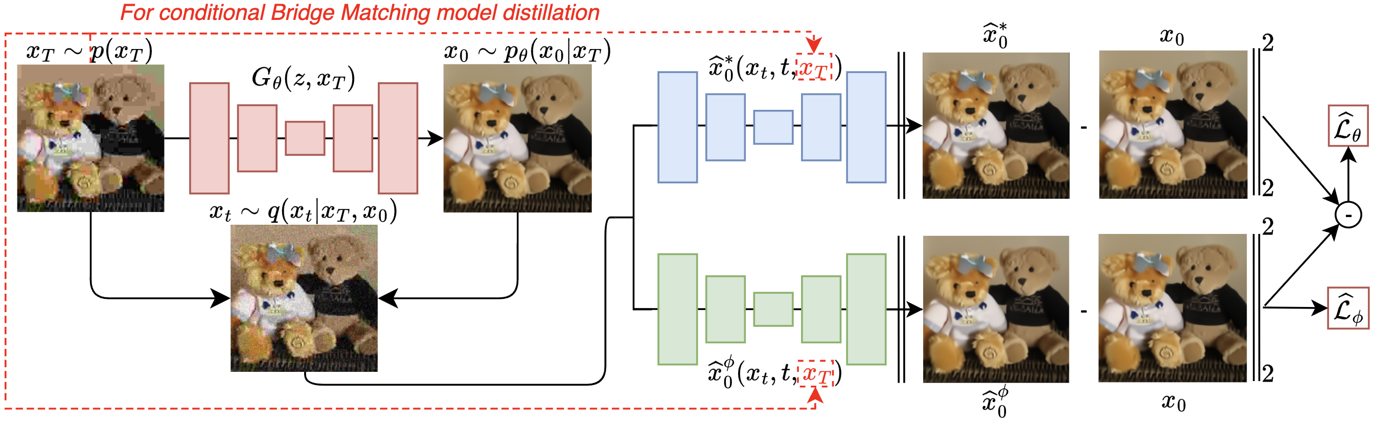
🔼 Figure 3 illustrates the Inverse Bridge Matching Distillation (IBMD) method. The goal is to create a fast, efficient generator that mimics a trained (conditional) Bridge Matching model. This generator, Gθ(z, xT), learns to produce samples from corrupted data p(xT). The key is defining a new coupling, pθ(x0, xT) = pθ(x0|xT)p(xT), using the generator. The method then aims to train the generator such that the Bridge Matching process using this new coupling yields the same output (x0) as the original, slower, teacher model. This is achieved by training the bridge model with the new coupling pθ(x0, xT) and then using a novel objective function from Theorem 3.2 to refine the generator Gθ.
read the caption
Figure 3: Overview of our method Inverse Bridge Matching Distillation (IBMD). The goal is to distill a trained (Conditional) Bridge Matching model into a generator Gθ(z,xT)subscript𝐺𝜃𝑧subscript𝑥𝑇G_{\theta}(z,x_{T})italic_G start_POSTSUBSCRIPT italic_θ end_POSTSUBSCRIPT ( italic_z , italic_x start_POSTSUBSCRIPT italic_T end_POSTSUBSCRIPT ), which learns to produce samples using the corrupted data p(xT)𝑝subscript𝑥𝑇p(x_{T})italic_p ( italic_x start_POSTSUBSCRIPT italic_T end_POSTSUBSCRIPT ). Generator Gθ(z,xT)subscript𝐺𝜃𝑧subscript𝑥𝑇G_{\theta}(z,x_{T})italic_G start_POSTSUBSCRIPT italic_θ end_POSTSUBSCRIPT ( italic_z , italic_x start_POSTSUBSCRIPT italic_T end_POSTSUBSCRIPT ) defines the coupling pθ(x0,xT)=pθ(x0|xT)p(xT)subscript𝑝𝜃subscript𝑥0subscript𝑥𝑇subscript𝑝𝜃conditionalsubscript𝑥0subscript𝑥𝑇𝑝subscript𝑥𝑇p_{\theta}(x_{0},x_{T})=p_{\theta}(x_{0}|x_{T})p(x_{T})italic_p start_POSTSUBSCRIPT italic_θ end_POSTSUBSCRIPT ( italic_x start_POSTSUBSCRIPT 0 end_POSTSUBSCRIPT , italic_x start_POSTSUBSCRIPT italic_T end_POSTSUBSCRIPT ) = italic_p start_POSTSUBSCRIPT italic_θ end_POSTSUBSCRIPT ( italic_x start_POSTSUBSCRIPT 0 end_POSTSUBSCRIPT | italic_x start_POSTSUBSCRIPT italic_T end_POSTSUBSCRIPT ) italic_p ( italic_x start_POSTSUBSCRIPT italic_T end_POSTSUBSCRIPT ) and we aim to learn the generator in such way that Bridge Matching with pθ(x0,xT)subscript𝑝𝜃subscript𝑥0subscript𝑥𝑇p_{\theta}(x_{0},x_{T})italic_p start_POSTSUBSCRIPT italic_θ end_POSTSUBSCRIPT ( italic_x start_POSTSUBSCRIPT 0 end_POSTSUBSCRIPT , italic_x start_POSTSUBSCRIPT italic_T end_POSTSUBSCRIPT ) produces the same (Conditional) Bridge Matching model x^0ϕ=x^0θsuperscriptsubscript^𝑥0italic-ϕsuperscriptsubscript^𝑥0𝜃\widehat{x}_{0}^{\phi}=\widehat{x}_{0}^{\theta}over^ start_ARG italic_x end_ARG start_POSTSUBSCRIPT 0 end_POSTSUBSCRIPT start_POSTSUPERSCRIPT italic_ϕ end_POSTSUPERSCRIPT = over^ start_ARG italic_x end_ARG start_POSTSUBSCRIPT 0 end_POSTSUBSCRIPT start_POSTSUPERSCRIPT italic_θ end_POSTSUPERSCRIPT. To do so, we learn a bridge model x^0ϕsuperscriptsubscript^𝑥0italic-ϕ\widehat{x}_{0}^{\phi}over^ start_ARG italic_x end_ARG start_POSTSUBSCRIPT 0 end_POSTSUBSCRIPT start_POSTSUPERSCRIPT italic_ϕ end_POSTSUPERSCRIPT using coupling pθsubscript𝑝𝜃p_{\theta}italic_p start_POSTSUBSCRIPT italic_θ end_POSTSUBSCRIPT in the same way as the teacher model was learned. Then, we use our novel objective given in Theorem 3.2 to update the generator model Gθsubscript𝐺𝜃G_{\theta}italic_G start_POSTSUBSCRIPT italic_θ end_POSTSUBSCRIPT.

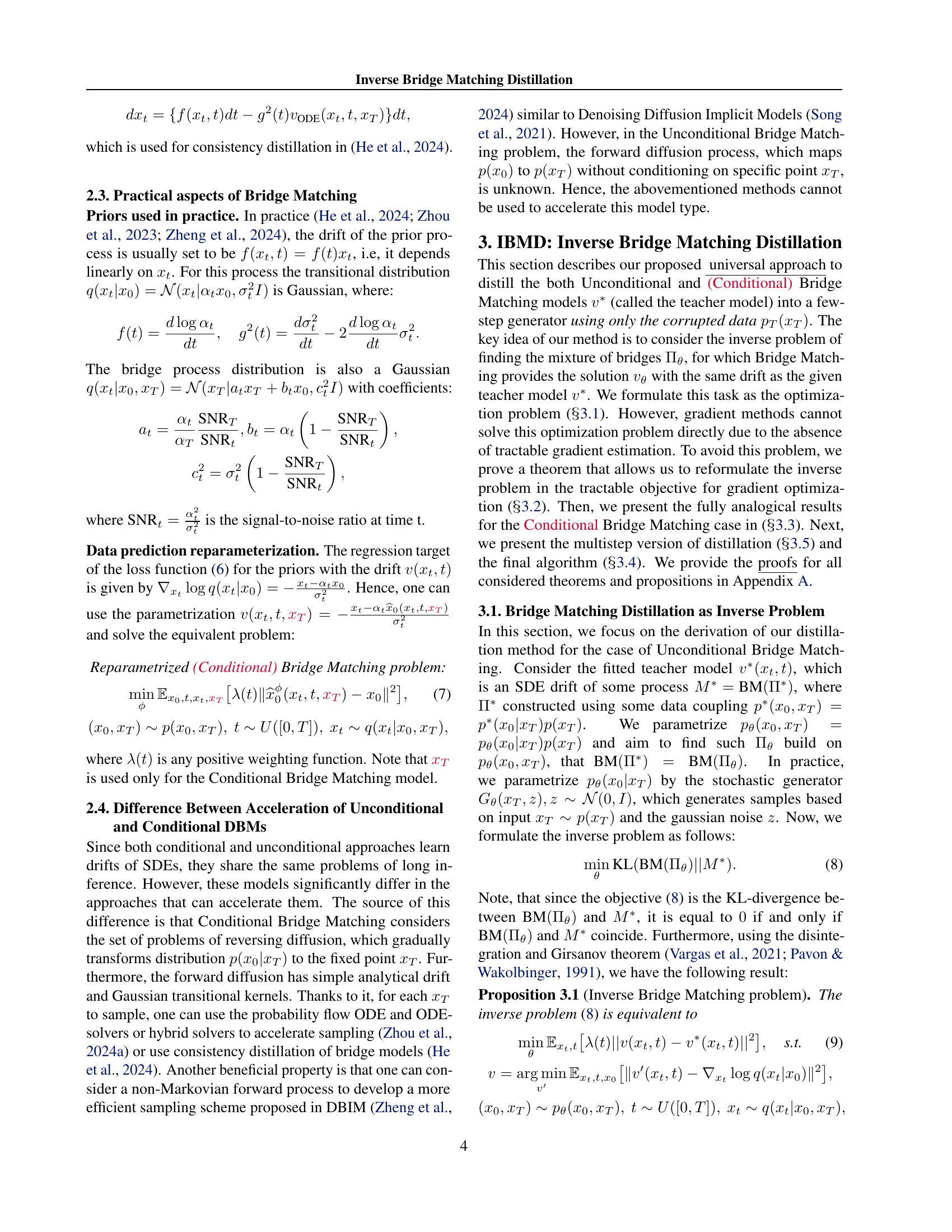
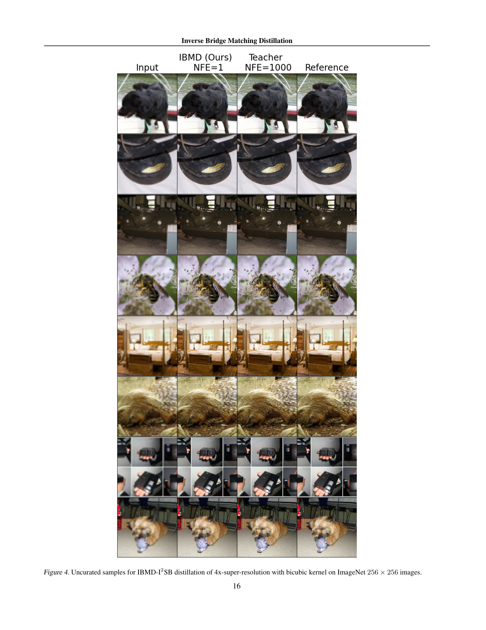
🔼 This figure displays the results of the Inverse Bridge Matching Distillation (IBMD) method applied to super-resolution. Specifically, it shows the results of using IBMD to distill a teacher model (trained with 1000 steps) into a student model capable of performing 4x super-resolution with only a single inference step (NFE=1). The images demonstrate examples of input images, outputs from the IBMD-I2SB model (ours), outputs from the teacher model (I2SB), and the ground truth (reference) images. The comparison allows for a visual assessment of the performance of the IBMD method in achieving high-quality super-resolution with significantly reduced computational cost.
read the caption
Figure 4: Uncurated samples for IBMD-I2SB distillation of 4x-super-resolution with bicubic kernel on ImageNet 256×256256256256\times 256256 × 256 images.

🔼 This figure showcases the results of Inverse Bridge Matching Distillation (IBMD) applied to a 4x super-resolution task using the I2SB model. The model is specifically trained with a pool kernel and evaluated on 256x256 ImageNet images. The image shows sets of input images, the results obtained using IBMD with only one forward pass (NFE=1), the results from the original I2SB model with 1000 forward passes (NFE=1000), and the ground truth (reference) images. This comparison highlights the significant speedup and comparable image quality achieved by IBMD compared to the original I2SB model.
read the caption
Figure 5: Uncurated samples for IBMD-I2SB distillation of 4x-super-resolution with pool kernel on ImageNet 256×256256256256\times 256256 × 256 images.

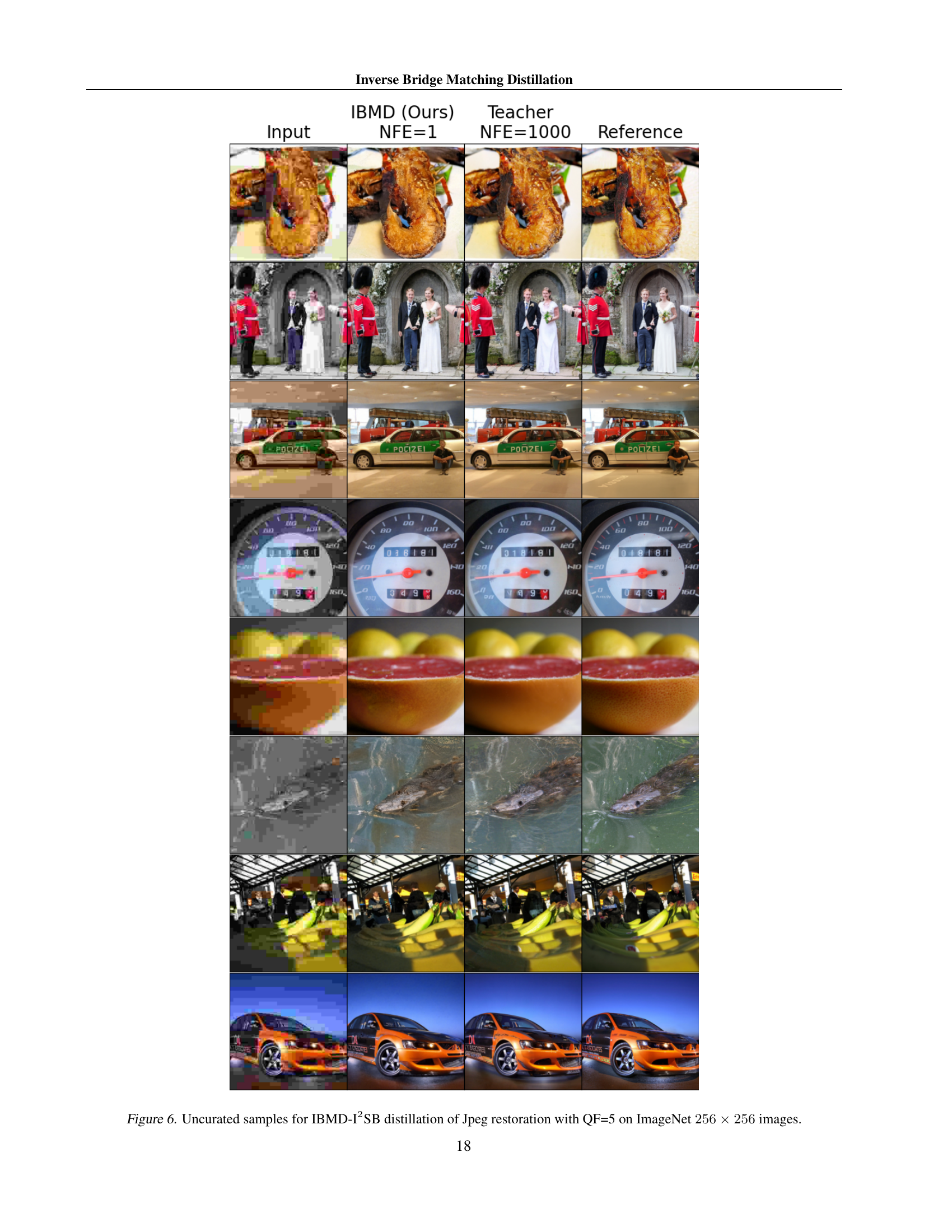
🔼 This figure displays the results of applying Inverse Bridge Matching Distillation (IBMD) to a pre-trained I2SB model for JPEG restoration. The task is to restore JPEG-compressed images with a quality factor (QF) of 5. The leftmost column shows the original, compressed images. The next three columns present the results of the IBMD model with only one forward pass (NFE=1), the original, pre-trained I2SB model (NFE=1000), and the ground truth (reference) images respectively. This visualization allows for a direct comparison of the restoration quality between the distilled model (IBMD) and the teacher model (I2SB), highlighting the improved efficiency (reduced number of forward diffusion steps) without substantial loss of image quality.
read the caption
Figure 6: Uncurated samples for IBMD-I2SB distillation of Jpeg restoration with QF=5 on ImageNet 256×256256256256\times 256256 × 256 images.

🔼 This figure displays the results of applying Inverse Bridge Matching Distillation (IBMD) to a pre-trained I2SB model (trained on ImageNet 256x256 images). The task was JPEG restoration with a quality factor (QF) of 10. The figure shows input images, the output of the IBMD model with 1 Noise-Free Expectation (NFE), the output of the original I2SB teacher model (with 1000 NFEs), and a reference image which is the ground truth clean image. This comparison illustrates the effectiveness of IBMD in accelerating inference (1 NFE compared to 1000 NFEs) while maintaining relatively high quality in the generated image. Each row represents a different image.
read the caption
Figure 7: Uncurated samples for IBMD-I2SB distillation of Jpeg restoration with QF=10 on ImageNet 256×256256256256\times 256256 × 256 images.

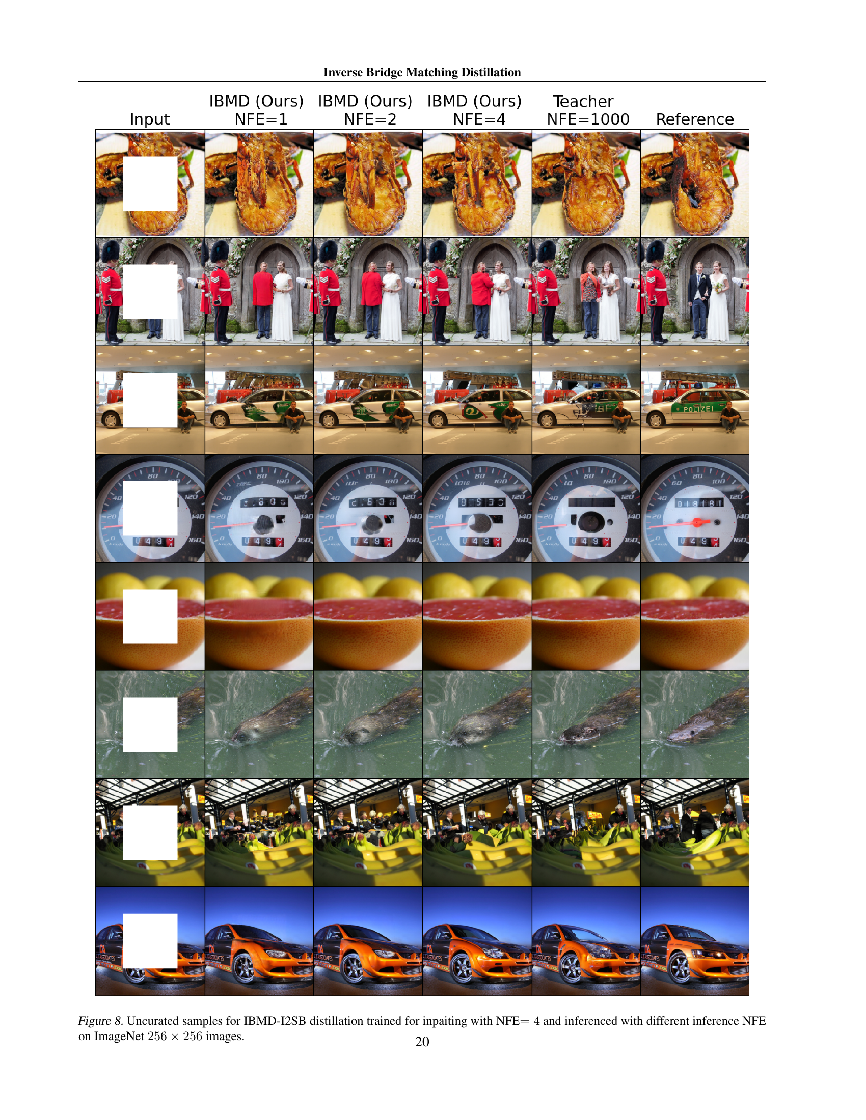
🔼 This figure displays uncurated samples from the Inverse Bridge Matching Distillation (IBMD) method applied to an I2SB (Image-to-Image Schrödinger Bridge) model. The model was initially trained for image inpainting using 4 noise free steps (NFE). The figure presents the results of inference using different numbers of NFEs (1, 2, and 4) to demonstrate the impact of reducing the number of inference steps on image quality. The results are compared to the original I2SB teacher model (1000 NFEs) and the corresponding reference images. The goal is to show how IBMD can successfully distill the teacher model while significantly speeding up the inference process.
read the caption
Figure 8: Uncurated samples for IBMD-I2SB distillation trained for inpaiting with NFE=4absent4=4= 4 and inferenced with different inference NFE on ImageNet 256×256256256256\times 256256 × 256 images.
🔼 This figure displays the results of inpainting using the IBMD-DDBM (Inverse Bridge Matching Distillation - Denoising Diffusion Bridge Model) method. The IBMD-DDBM model was initially trained with 4 noise-free encoding steps (NFE). The figure shows inpainting results for different numbers of inference steps (NFE) during the testing phase (1, 2, and 4 NFEs) alongside the results from the original teacher model (NFE=500) and the ground truth (reference) images. All images are from the ImageNet dataset with a resolution of 256x256 pixels. This visual comparison allows assessment of the trade-off between speed (lower NFE) and quality of inpainting against the teacher and reference images.
read the caption
Figure 9: Uncurated samples for IBMD-DDBM distillation trained for inpaiting with NFE=4absent4=4= 4 and inferenced with different inference NFE on ImageNet 256×256256256256\times 256256 × 256 images.

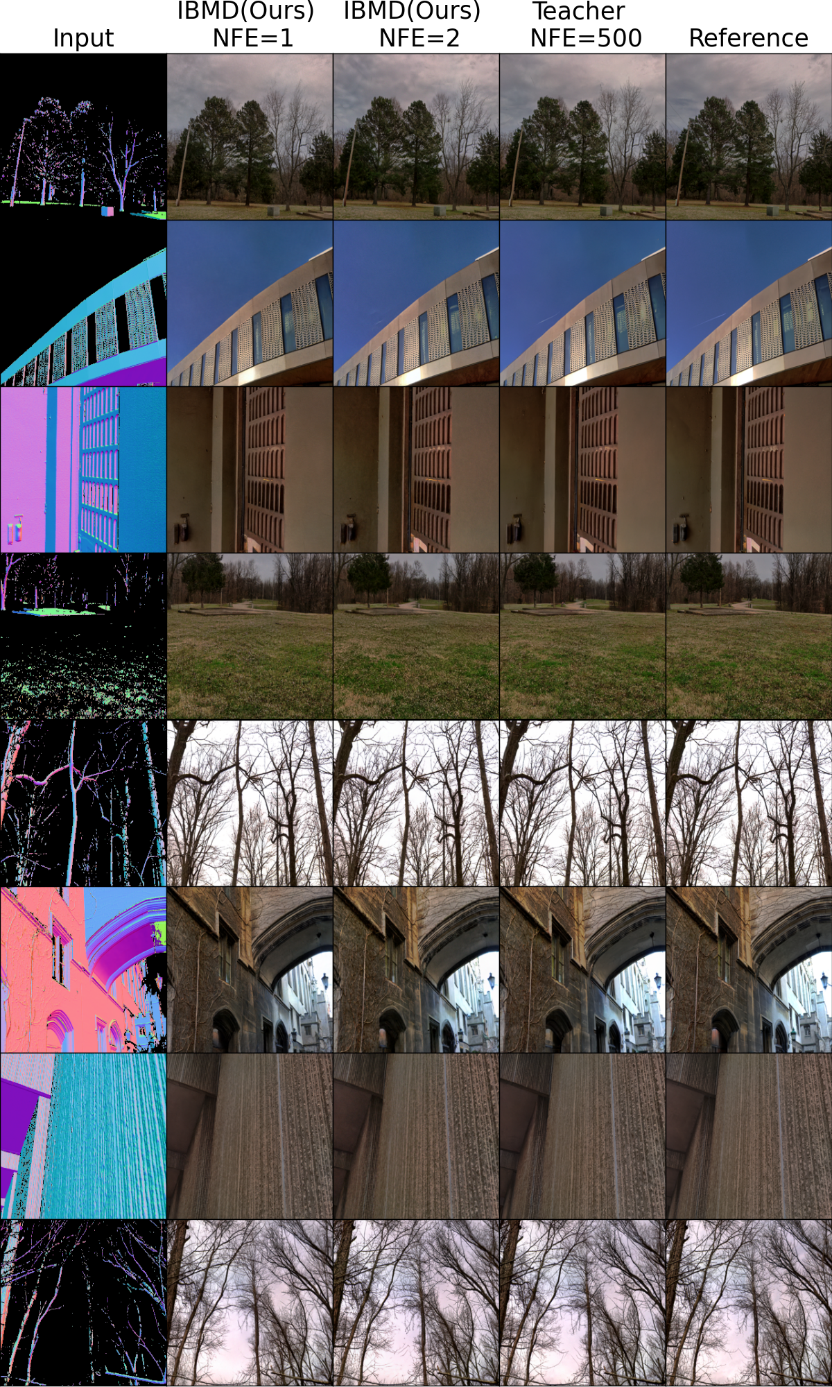
🔼 This figure displays the results of the Inverse Bridge Matching Distillation (IBMD) method applied to a Denoising Diffusion Bridge Model (DDBM). Specifically, it shows uncurated samples generated by IBMD models trained with different numbers of function evaluations (NFEs). Two IBMD models are compared: one trained with 2 NFEs and another with 1 NFE. These are compared against the corresponding results from the original, teacher DDBM (trained with 500 NFEs) and the reference images. The images are all from the DIODE-Outdoor dataset (resolution 256x256). The samples generated using the IBMD approach demonstrate the ability of the method to accelerate DDBM inference significantly while maintaining a similar generation quality compared to the teacher model, especially for the model trained with 2 NFEs.
read the caption
Figure 10: Uncurated samples from IBMD-DDBM distillation trained on the DIODE-Outdoor dataset (256×256256256256\times 256256 × 256) with NFE=2absent2=2= 2 and NFE=1absent1=1= 1, inferred using the corresponding NFEs on the training set.

🔼 This figure displays uncurated samples generated from the IBMD-DDBM model. The model was trained on the DIODE-Outdoor dataset, which contains images with a resolution of 256x256 pixels. Two versions of the model are shown, one trained with 2 Noise-Free Evaluations (NFEs) and another with 1 NFE. The results demonstrate the model’s performance on unseen test data, showcasing its ability to generate realistic and high-quality images from noisy or incomplete inputs, even with a reduced number of NFEs during inference. Each row compares the input image (leftmost column) with the outputs from the 1-NFE and 2-NFE IBMD models, followed by the teacher model and the ground truth reference image.
read the caption
Figure 11: Uncurated samples from IBMD-DDBM distillation trained on the DIODE-Outdoor dataset (256×256256256256\times 256256 × 256) with NFE=2absent2=2= 2 and NFE=1absent1=1= 1, inferred using the corresponding NFEs on the test set.

🔼 This figure displays the results of the Inverse Bridge Matching Distillation (IBMD) method applied to the Edges to Handbags dataset. The IBMD technique was trained using the Denoising Diffusion Bridge Model (DDBM). Two versions of the IBMD model are presented: one trained with 2 Noise Free Ensembles (NFE) and another with 1 NFE. Samples generated by each IBMD model are shown alongside those generated by the original DDBM teacher model (with 500 NFEs) and the corresponding reference images from the dataset. This comparison showcases the ability of the IBMD method to produce comparable results to a much more computationally expensive model, using far fewer NFEs. The images demonstrate different handbag styles with their corresponding outlines. The results are from the training set.
read the caption
Figure 12: Uncurated samples from IBMD-DDBM distillation trained on the Edges →→\rightarrow→ Handbags dataset (64×64646464\times 6464 × 64) with NFE=2absent2=2= 2 and NFE=1absent1=1= 1, inferred using the corresponding NFEs on the training set.
More on tables
| 4 super-resolution (bicubic) | ImageNet (256 256) | ||
| NFE | FID | CA | |
| DDRM (Kawar et al., 2022) | 20 | 21.3 | 63.2 |
| DDNM (Wang et al., 2023) | 100 | 13.6 | 65.5 |
| GDM (Song et al., 2023) | 100 | 3.6 | 72.1 |
| ADM (Dhariwal & Nichol, 2021) | 1000 | 14.8 | 66.7 |
| CDSB (Shi et al., 2022) | 50 | 13.6 | 61.0 |
| I2SB (Liu et al., 2023a) | 1000 | 2.8 | 70.7 |
| IBMD-I2SB (Ours) | 1 | 2.5 | 72.4 |
🔼 This table presents a quantitative comparison of different diffusion models on the task of JPEG image restoration, specifically using a quality factor (QF) of 5. It shows the Fréchet Inception Distance (FID) and Classifier Accuracy (CA) scores achieved by various methods, including DDRM, IGDM, Palette, CDSB, I2SB, and the proposed IBMD method. The FID score measures the discrepancy between the generated image distribution and the real image distribution, with lower scores being better, while CA measures the accuracy of a classifier in distinguishing between generated and real images, with higher scores being preferable. The number of function evaluations (NFE) needed for inference is also reported, indicating the computational efficiency of each method. I2SB (Liu et al., 2023a) provides baseline results for comparison. The table enables assessing the performance improvements attained by the proposed method in terms of FID, CA, and NFE.
read the caption
Table 2: Results on the image JPEG restoration task with QF=5. Baseline results are taken from I2SB (Liu et al., 2023a).
| JPEG restoration, QF. | ImageNet (256 256) | ||
| NFE | FID | CA | |
| DDRM (Kawar et al., 2022) | 20 | 28.2 | 53.9 |
| GDM (Song et al., 2023) | 100 | 8.6 | 64.1 |
| Palette (Saharia et al., 2022) | 1000 | 8.3 | 64.2 |
| CDSB (Shi et al., 2022) | 50 | 38.7 | 45.7 |
| I2SB (Liu et al., 2023a) | 1000 | 4.6 | 67.9 |
| I2SB (Liu et al., 2023a) | 100 | 5.4 | 67.5 |
| IBMD-I2SB (Ours) | 1 | 5.3 | 67.2 |
🔼 Table 3 presents a comparison of different models on an image super-resolution task. It shows the Fréchet Inception Distance (FID) scores and Classifier Accuracy (CA) for various methods, including those proposed in the paper. The number of forward diffusion steps (NFE) required for inference is also indicated. The table highlights the performance improvement achieved by the proposed method (IBMD-I2SB) compared to existing state-of-the-art techniques. The baseline results are sourced from the I2SB paper (Liu et al., 2023a). This allows for a direct comparison to demonstrate the efficiency gains of the proposed technique.
read the caption
Table 3: Results on the image super-resolution task. Baseline results are taken from I2SB (Liu et al., 2023a).
| 4 super-resolution (pool) | ImageNet (256 256) | ||
| NFE | FID | CA | |
| DDRM (Kawar et al., 2022) | 20 | 14.8 | 64.6 |
| DDNM (Wang et al., 2023) | 100 | 9.9 | 67.1 |
| GDM (Song et al., 2023) | 100 | 3.8 | 72.3 |
| ADM (Dhariwal & Nichol, 2021) | 1000 | 3.1 | 73.4 |
| CDSB (Shi et al., 2022) | 50 | 13.0 | 61.3 |
| I2SB (Liu et al., 2023a) | 1000 | 2.7 | 71.0 |
| IBMD-I2SB (Ours) | 1 | 2.6 | 72.7 |
🔼 This table presents a comparison of different diffusion models’ performance on the task of JPEG image restoration, specifically using quality factor 10 (QF=10). It shows the Fréchet Inception Distance (FID) score and Classifier Accuracy (CA) achieved by various models, including DDRM, IGDM, Palette, CDSB, I2SB, and the proposed IBMD method. Lower FID indicates better image quality, and higher CA represents better classification accuracy. The Number of Forward Euler Steps (NFE) required for each method is also displayed, reflecting the computational cost. Baseline results are included for comparison, sourced from the I2SB method in a prior publication by Liu et al. (2023a). This helps highlight the effectiveness of the IBMD model in achieving similar quality with significantly reduced computational expense.
read the caption
Table 4: Results on the image JPEG restoration task with QF=10. Baseline results are taken from I2SB (Liu et al., 2023a).
| JPEG restoration, QF. | ImageNet (256 256) | ||
| NFE | FID | CA | |
| DDRM (Kawar et al., 2022) | 20 | 16.7 | 64.7 |
| GDM (Song et al., 2023) | 100 | 6.0 | 71.0 |
| Palette (Saharia et al., 2022) | 1000 | 5.4 | 70.7 |
| CDSB (Shi et al., 2022) | 50 | 18.6 | 60.0 |
| I2SB (Liu et al., 2023a) | 1000 | 3.6 | 72.1 |
| I2SB (Liu et al., 2023a) | 100 | 4.4 | 71.6 |
| IBMD-I2SB (Ours) | 1 | 3.8 | 72.4 |
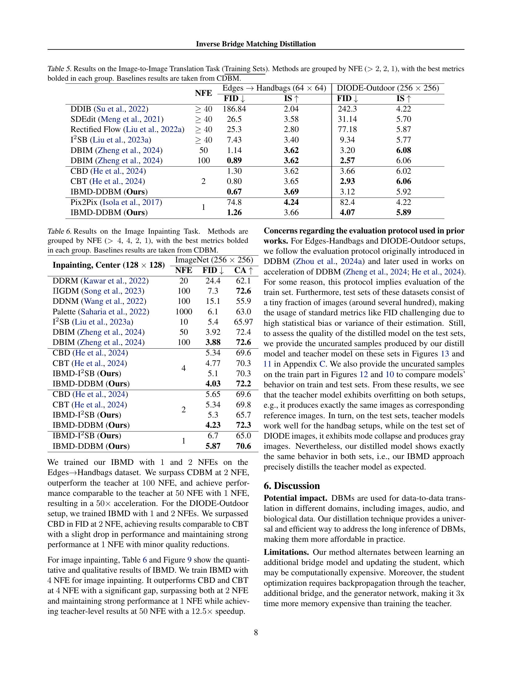
🔼 Table 5 presents results for image-to-image translation tasks using various methods, categorized by the number of forward diffusion steps (NFE). The table compares different models’ performance on two datasets: Edges to Handbags (64x64 resolution) and DIODE-Outdoor (256x256 resolution). Performance is evaluated using FID (Fréchet Inception Distance) and IS (Inception Score), with lower FID indicating better image quality and higher IS also signifying better image quality. The models are grouped into categories based on their NFE values (>2, 2, 1), allowing for easy comparison within similar inference complexity groups. The best results within each NFE group are highlighted in bold. Baseline results from the CDBM method are included for comparison. This enables a comprehensive evaluation of different approaches across varying computational costs, showcasing the effectiveness of different methods at generating high-quality image translations.
read the caption
Table 5: Results on the Image-to-Image Translation Task (Training Sets). Methods are grouped by NFE (>2absent2>2> 2, 2222, 1111), with the best metrics bolded in each group. Baselines results are taken from CDBM.
| NFE | Edges Handbags (64 64) | DIODE-Outdoor (256 256) | |||
| FID | IS | FID | IS | ||
| DDIB (Su et al., 2022) | 186.84 | 2.04 | 242.3 | 4.22 | |
| SDEdit (Meng et al., 2021) | 26.5 | 3.58 | 31.14 | 5.70 | |
| Rectified Flow (Liu et al., 2022a) | 25.3 | 2.80 | 77.18 | 5.87 | |
| SB (Liu et al., 2023a) | 7.43 | 3.40 | 9.34 | 5.77 | |
| DBIM (Zheng et al., 2024) | 50 | 1.14 | 3.62 | 3.20 | 6.08 |
| DBIM (Zheng et al., 2024) | 100 | 0.89 | 3.62 | 2.57 | 6.06 |
| CBD (He et al., 2024) | 2 | 1.30 | 3.62 | 3.66 | 6.02 |
| CBT (He et al., 2024) | 0.80 | 3.65 | 2.93 | 6.06 | |
| IBMD-DDBM (Ours) | 0.67 | 3.69 | 3.12 | 5.92 | |
| Pix2Pix (Isola et al., 2017) | 1 | 74.8 | 4.24 | 82.4 | 4.22 |
| IBMD-DDBM (Ours) | 1.26 | 3.66 | 4.07 | 5.89 | |
🔼 Table 6 presents the results of image inpainting experiments. Several methods are compared, categorized by the number of function evaluations (NFEs) they used. The methods are grouped into categories based on their NFE count (>4, 4, 2, 1), allowing for a comparison of performance across different computational budgets. For each group, the best performance in terms of FID (Fréchet Inception Distance) and CA (Classifier Accuracy) is highlighted in bold. Baseline results from the CDBM (Conditional Bridge Matching) method are included for reference. This provides a comprehensive view of the trade-off between computational cost and inpainting quality for various algorithms.
read the caption
Table 6: Results on the Image Inpainting Task. Methods are grouped by NFE (>4absent4>4> 4, 4444, 2222, 1111), with the best metrics bolded in each group. Baselines results are taken from CDBM.
| Inpainting, Center (128 128) | ImageNet (256 256) | ||
| NFE | FID | CA | |
| DDRM (Kawar et al., 2022) | 20 | 24.4 | 62.1 |
| GDM (Song et al., 2023) | 100 | 7.3 | 72.6 |
| DDNM (Wang et al., 2022) | 100 | 15.1 | 55.9 |
| Palette (Saharia et al., 2022) | 1000 | 6.1 | 63.0 |
| I2SB (Liu et al., 2023a) | 10 | 5.4 | 65.97 |
| DBIM (Zheng et al., 2024) | 50 | 3.92 | 72.4 |
| DBIM (Zheng et al., 2024) | 100 | 3.88 | 72.6 |
| CBD (He et al., 2024) | 4 | 5.34 | 69.6 |
| CBT (He et al., 2024) | 4.77 | 70.3 | |
| IBMD-I2SB (Ours) | 5.1 | 70.3 | |
| IBMD-DDBM (Ours) | 4.03 | 72.2 | |
| CBD (He et al., 2024) | 2 | 5.65 | 69.6 |
| CBT (He et al., 2024) | 5.34 | 69.8 | |
| IBMD-I2SB (Ours) | 5.3 | 65.7 | |
| IBMD-DDBM (Ours) | 4.23 | 72.3 | |
| IBMD-I2SB (Ours) | 1 | 6.7 | 65.0 |
| IBMD-DDBM (Ours) | 5.87 | 70.6 | |
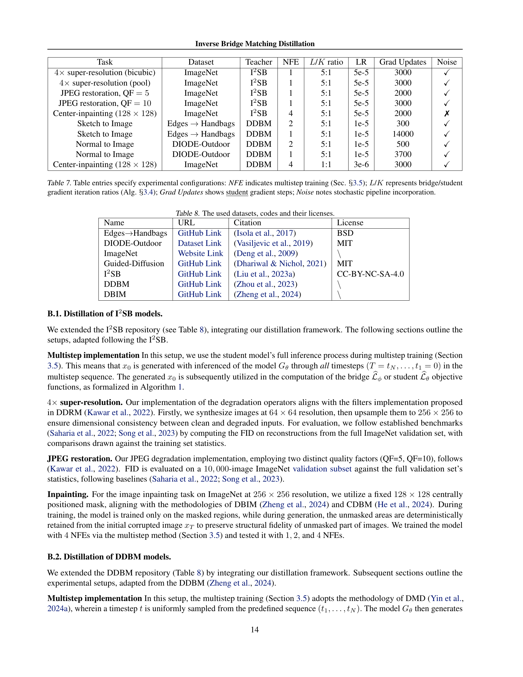
🔼 Table 7 details the experimental setup used in the paper. It lists the specific configurations for each experiment, making it easy to understand and reproduce the results. For each task, it specifies the dataset used, the teacher model employed, the number of forward diffusion steps (NFE) in the teacher model, the ratio of bridge to student gradient iterations (L/K), the learning rate (LR) used, the number of student gradient updates performed during training, and whether a stochastic pipeline was incorporated. This level of detail ensures reproducibility and allows readers to comprehend the design choices behind the experiments.
read the caption
Table 7: Table entries specify experimental configurations: NFE indicates multistep training (Sec. \wasyparagraph3.5); L𝐿Litalic_L/K𝐾Kitalic_K represents bridge/student gradient iteration ratios (Alg. \wasyparagraph3.4); Grad Updates shows student gradient steps; Noise notes stochastic pipeline incorporation.
| Task | Dataset | Teacher | NFE | / ratio | LR | Grad Updates | Noise |
| super-resolution (bicubic) | ImageNet | I2SB | 1 | 5:1 | 5e-5 | 3000 | ✓ |
| super-resolution (pool) | ImageNet | I2SB | 1 | 5:1 | 5e-5 | 3000 | ✓ |
| JPEG restoration, QF | ImageNet | I2SB | 1 | 5:1 | 5e-5 | 2000 | ✓ |
| JPEG restoration, QF | ImageNet | I2SB | 1 | 5:1 | 5e-5 | 3000 | ✓ |
| Center-inpainting () | ImageNet | I2SB | 4 | 5:1 | 5e-5 | 2000 | ✗ |
| Sketch to Image | Edges Handbags | DDBM | 2 | 5:1 | 1e-5 | 300 | ✓ |
| Sketch to Image | Edges Handbags | DDBM | 1 | 5:1 | 1e-5 | 14000 | ✓ |
| Normal to Image | DIODE-Outdoor | DDBM | 2 | 5:1 | 1e-5 | 500 | ✓ |
| Normal to Image | DIODE-Outdoor | DDBM | 1 | 5:1 | 1e-5 | 3700 | ✓ |
| Center-inpainting () | ImageNet | DDBM | 4 | 1:1 | 3e-6 | 3000 | ✓ |
🔼 This table lists the datasets used in the experiments of the paper, along with links to their code repositories and the associated licenses.
read the caption
Table 8: The used datasets, codes and their licenses.
Full paper#