TL;DR#
Current generative models like diffusion models are excellent but computationally expensive. Consistency models are faster, but their performance in the high-dimensional latent space (crucial for applications like text-to-image generation) lags. This paper tackles this problem. The authors found that latent data has many outliers which negatively impact the training of consistency models.
The proposed solution uses a new loss function (Cauchy loss) to handle outliers effectively. They also introduce several techniques such as the use of diffusion loss in early training stages and optimal transport to improve training stability and efficiency. These novel techniques significantly improve the performance of consistency models, making them closer to that of diffusion models. The improved model is tested on several datasets, proving its efficacy.
Key Takeaways#
Why does it matter?#
This paper is important because it significantly improves the performance of latent consistency models, a new family of generative models. Addressing the limitations of current methods in handling high-dimensional latent data, this work directly contributes to advancing the field of generative modeling by making latent consistency models more efficient and scalable for large-scale tasks. The proposed techniques are readily applicable to various applications, including text-to-image and video generation, opening new avenues for research and development in these areas.
Visual Insights#

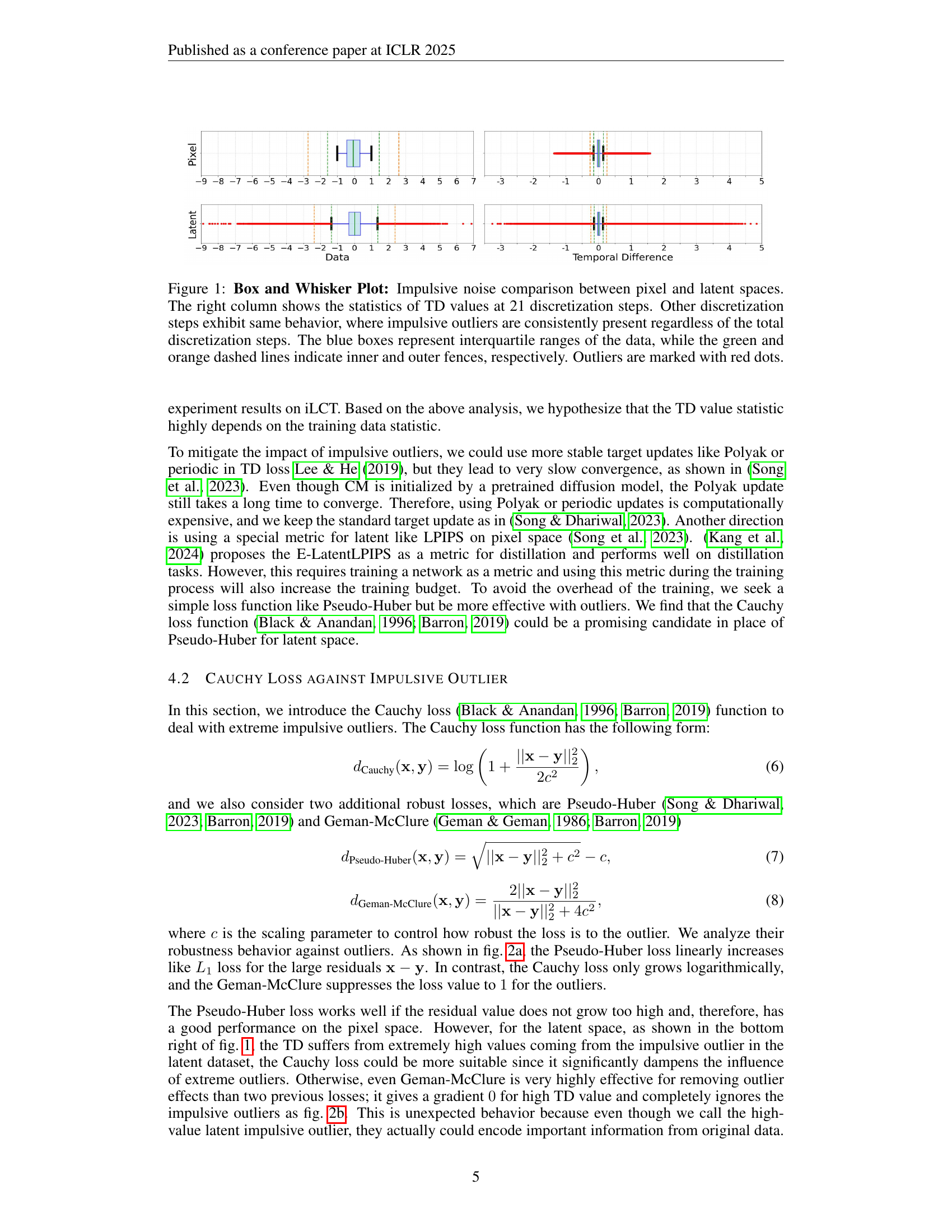
🔼 This figure uses box and whisker plots to compare the distribution of data and temporal difference (TD) values in pixel and latent spaces. The left side shows the distribution of data values in each space, highlighting the presence of extreme outliers (marked in red) in the latent space. These outliers are much more pronounced in the latent space compared to the pixel space. The right side displays the distribution of TD values (calculated at one point in the training process, specifically timestep 21 of a total of 36). Again, the latent space shows a substantially higher concentration and magnitude of outliers in the TD values. The box and whisker plots clearly show that the range of TD values, the interquartile range, and the presence of extreme values differ greatly between the pixel and latent spaces. This difference helps explain why existing consistency training methods perform poorly in latent space due to the significant impact of these impulsive outliers on the loss function.
read the caption
Figure 1: Box and Whisker Plot: Impulsive noise comparison between pixel and latent spaces. The right column shows the statistics of TD values at 21 discretization steps. Other discretization steps exhibit same behavior, where impulsive outliers are consistently present regardless of the total discretization steps. The blue boxes represent interquartile ranges of the data, while the green and orange dashed lines indicate inner and outer fences, respectively. Outliers are marked with red dots.
| Model NFE FID Recall Epochs Total Bs Pixel Diffusion Model WaveDiff (Phung et al., 2023) 2 5.94 0.37 500 64 Score SDE (Song et al., 2020) 4000 7.23 - 6.2K - DDGAN (Xiao et al., 2021) 2 7.64 0.36 800 32 RDUOT (Dao et al., 2023b) 2 5.60 0.38 600 24 RDM (Teng et al., 2023) 270 3.15 0.55 4K - UNCSN++ (Kim et al., 2021) 2000 7.16 - - - Latent Diffusion Model LFM-8 (Dao et al., 2023a) 85 5.82 0.41 500 112 LDM-4 (Rombach et al., 2021) 200 5.11 0.49 600 48 LSGM (Vahdat et al., 2021) 23 7.22 - 1K - DDMI (Park et al., 2024) 1000 7.25 - - - DIMSUM (Phung et al., 2024) 73 3.76 0.56 395 32 250 8.85 - 1.4K 128 Latent Consistency Model iLCT (Song & Dhariwal, 2023) 1 37.15 0.12 1.4K 128 iLCT (Song & Dhariwal, 2023) 2 16.84 0.24 1.4K 128 Ours 1 7.27 0.50 1.4K 128 Ours 2 6.93 0.52 1.4K 128 (a) CelebA-HQ Model NFE FID Recall Epochs Total Bs Pixel Diffusion Model WaveDiff (Phung et al., 2023) 2 5.94 0.37 500 64 Score SDE (Song et al., 2020) 4000 7.23 - 6.2K - DDGAN (Xiao et al., 2021) 2 5.25 0.36 500 32 Latent Diffusion Model LFM-8 (Dao et al., 2023a) 90 7.70 0.39 90 112 LDM-8 (Rombach et al., 2021) 400 4.02 0.52 400 96 250 10.81 - 1.8K 256 Latent Consistency Model iLCT (Song & Dhariwal, 2023) 1 52.45 0.11 1.8K 256 iLCT (Song & Dhariwal, 2023) 2 24.67 0.17 1.8K 256 Ours 1 8.87 0.47 1.8K 256 Ours 2 7.71 0.48 1.8K 256 (b) LSUN Church Model NFE FID Recall Epochs Total Bs Latent Diffusion Model LFM-8 (Dao et al., 2023a) 84 8.07 0.40 700 128 LDM-4 (Rombach et al., 2021) 200 4.98 0.50 400 42 250 10.23 - 1.4K 128 Latent Consistency Model iLCT (Song & Dhariwal, 2023) 1 48.82 0.15 1.4K 128 iLCT (Song & Dhariwal, 2023) 2 21.15 0.19 1.4K 128 Ours 1 8.72 0.42 1.4K 128 Ours 2 8.29 0.43 1.4K 128 (c) FFHQ |
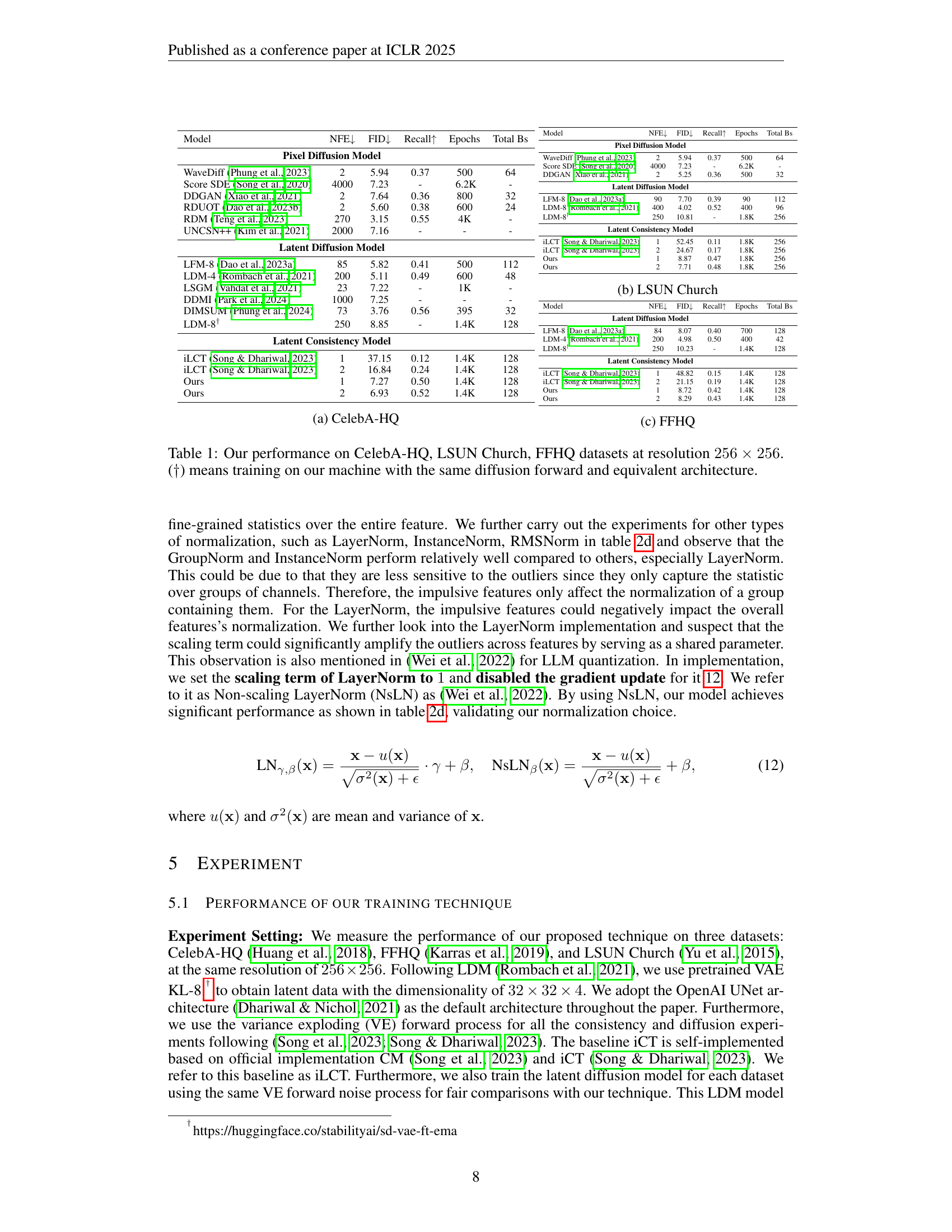
🔼 Table 1 presents a comparison of the performance of different generative models on three benchmark datasets: CelebA-HQ, LSUN Church, and FFHQ. All models were evaluated at a resolution of 256x256 pixels. The table shows key metrics including FID (Fréchet Inception Distance), Recall, and the number of function evaluations (NFEs) required for image generation. The models compared include various diffusion models and the latent consistency model proposed in the paper, both using one and two sampling steps. This allows for assessing the quality and efficiency of each method across different datasets. The ‘+†’ symbol indicates that a model was trained on the author’s machine using the same diffusion forward process and equivalent architecture as the other models for fair comparison. The goal is to showcase the improved performance of the proposed latent consistency model training technique.
read the caption
Table 1: Our performance on CelebA-HQ, LSUN Church, FFHQ datasets at resolution 256×256256256256\times 256256 × 256. (††\dagger†) means training on our machine with the same diffusion forward and equivalent architecture.
In-depth insights#
Latent Space Outliers#
The concept of ‘Latent Space Outliers’ in generative models is critical because latent spaces, while offering advantages for scalability, often harbor data points significantly deviating from the norm. These outliers, invisible in the original data, can severely hinder the training of consistency models, leading to poor performance. The paper highlights the crucial difference in the statistical properties between pixel and latent spaces, revealing that latent spaces tend to contain high-magnitude, impulsive outliers which act like noise and disrupt the training process. Addressing these outliers is crucial, as standard methods for handling outliers in pixel space prove inadequate. The use of robust loss functions, such as the Cauchy loss, is proposed to mitigate the effect of outliers, showing superior performance compared to other methods like Pseudo-Huber Loss. Combining this with techniques like early timestep diffusion loss and optimal transport (OT) coupling, further enhances model robustness and efficiency. This approach significantly improves the performance of consistency training in the latent space, highlighting the importance of data analysis and tailored training strategies for optimal results in high-dimensional generative modeling.
Cauchy Loss Benefit#
The paper investigates the effectiveness of Cauchy loss in handling impulsive outliers present in latent space during the training of consistency models. Cauchy loss demonstrates robustness to extreme outliers, unlike the Pseudo-Huber loss which struggles with very high values. This robustness is crucial because latent spaces, often used in large-scale generative modeling (like text-to-image), tend to contain such outliers. The authors show that Cauchy loss significantly improves model performance, reducing the FID (Fréchet Inception Distance), a common metric for assessing the quality of generated images, and increasing Recall. The use of Cauchy loss is especially valuable in latent consistency training due to its resistance to the effects of outlier data points, bridging a performance gap between the model and more established diffusion models. The core benefit lies in its ability to maintain valuable information present in these extreme outlier values, unlike methods that harshly penalize or completely ignore them.
Diffusion Loss Aid#
A hypothetical ‘Diffusion Loss Aid’ section in a research paper on generative models would likely explore the use of diffusion-based loss functions to improve training. This approach might involve adding a diffusion loss term to the primary loss function (e.g., consistency loss), aiming to regularize the training process and enhance the model’s ability to generate high-quality samples. The section would delve into the theoretical underpinnings of combining diffusion losses with other loss types, such as exploring the interplay between forward and reverse diffusion processes. Empirical studies would be crucial, demonstrating the impact of different diffusion loss implementations (e.g., various weighting schemes, early vs. late timestep application) on the model’s performance (FID, Inception Score). Ablation experiments comparing models trained with and without diffusion loss would showcase the added benefit. An ideal paper would also investigate and explain the effect of hyperparameters associated with the diffusion loss on both the quality and efficiency of the training process. Finally, any potential drawbacks or limitations of incorporating this ‘Diffusion Loss Aid’ approach should also be discussed, for example, increased computational costs or potential negative impacts on training stability.
Adaptive Scaling#
Adaptive scaling, in the context of training generative models, is a crucial technique for managing the robustness and stability of the learning process. It dynamically adjusts hyperparameters, such as the scaling factor in robust loss functions, based on the characteristics of the data and the training progress. This adaptive approach contrasts with fixed-value scaling, which can lead to suboptimal performance and instability, especially when dealing with datasets containing impulsive outliers, as frequently seen in latent spaces. The benefits of adaptive scaling are significant: improved model performance, enhanced robustness to outliers, and faster convergence. By responding to the nuances of the data, the training avoids the pitfalls of a one-size-fits-all approach, ultimately leading to models that are more effective, efficient, and resilient to noisy or irregular data inputs. Careful design of the adaptive strategy is essential, however, to avoid introducing instability or other unforeseen issues. A well-designed adaptive scaling mechanism will smoothly adjust the scaling parameter based on a pre-defined strategy or feedback mechanism, allowing the model to efficiently navigate complex training landscapes.
NsLN Improves CT#
The heading ‘NsLN Improves CT’ suggests that Non-scaling Layer Normalization (NsLN) enhances the performance of Consistency Training (CT). NsLN likely addresses a critical limitation of CT in latent space, where the presence of outliers significantly degrades performance. Standard Layer Normalization, by considering the entire feature distribution, is unduly influenced by these outliers. NsLN mitigates this by removing the scaling term, preventing outlier amplification and enabling a more stable training process. This improvement is particularly vital when dealing with latent representations, which frequently contain impulsive noise. The enhanced robustness from NsLN allows the CT model to better capture the feature statistics and refine the model’s ability to reconstruct clean data from noisy samples. This leads to higher-quality image generation, even with only one or two sampling steps. The overall implication is that NsLN is a crucial architectural modification enabling successful scaling of consistency training to large-scale datasets, particularly beneficial in text-to-image and video generation tasks.
More visual insights#
More on figures

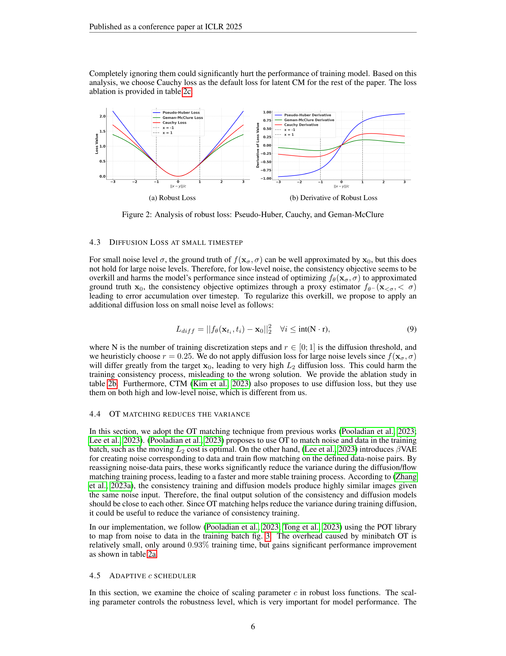
🔼 The figure illustrates a comparison of three robust loss functions: Pseudo-Huber, Cauchy, and Geman-McClure. The left subplot (a) shows the loss values plotted against the residual (||x - y||/c), demonstrating how each loss function handles outliers. The right subplot (b) displays the derivatives of these loss functions, highlighting their sensitivity to outliers. The Pseudo-Huber loss shows linear growth for large residuals, while the Cauchy loss exhibits logarithmic growth, and the Geman-McClure loss approaches a constant value. These differences in behavior indicate varying degrees of robustness to outliers, with the Cauchy loss offering a balance between robustness and sensitivity to informative outliers.
read the caption
(a) Robust Loss

🔼 The plot shows the derivative of three different robust loss functions: Pseudo-Huber, Cauchy, and Geman-McClure. The x-axis represents the normalized residual (||x-y||/c), and the y-axis represents the derivative of the loss function. The plot visually compares the sensitivity of each loss function to outliers (large residuals). The Cauchy loss shows a logarithmic increase with increasing residuals, demonstrating robustness to large outliers. The Pseudo-Huber loss shows a linear increase for larger residuals, while the Geman-McClure loss exhibits a sharp decrease to near zero for large residuals, indicating it will tend to ignore outliers.
read the caption
(b) Derivative of Robust Loss

🔼 This figure compares three robust loss functions: Pseudo-Huber, Cauchy, and Geman-McClure. Subfigure (a) shows the loss value as a function of the residual error (||x-y||/c) for each loss function, illustrating their different sensitivities to outliers. The Pseudo-Huber loss behaves linearly for large residuals, while the Cauchy loss increases logarithmically and the Geman-McClure loss plateaus at 1. Subfigure (b) presents the derivative of the loss function for each method, further clarifying the behavior of the loss in relation to the residual error and highlighting their different robustness properties when dealing with outliers.
read the caption
Figure 2: Analysis of robust loss: Pseudo-Huber, Cauchy, and Geman-McClure

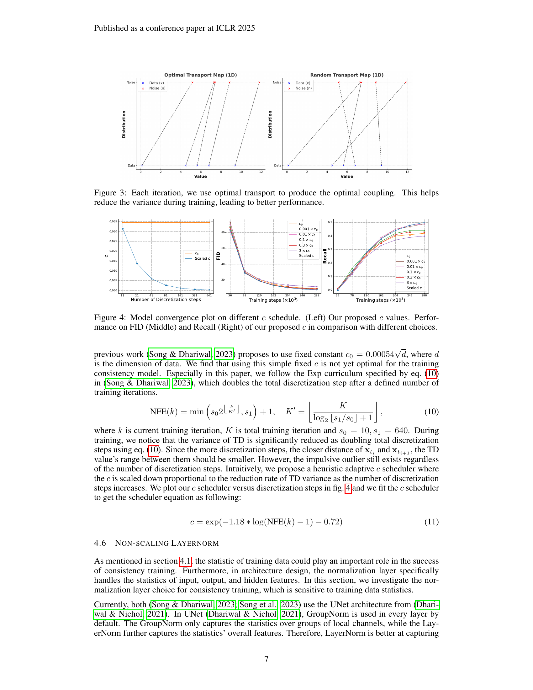
🔼 This figure demonstrates the use of optimal transport (OT) to improve the efficiency and stability of the consistency training process. Optimal transport is used to find the best mapping (coupling) between the noise and data distributions in each training iteration. This optimal coupling minimizes a cost function, effectively reducing the variance during training. By reducing variance, the training process becomes more stable, and ultimately leads to better model performance (as measured by metrics like FID and recall). The visualization likely shows the transport map, illustrating the flow from the noise distribution to the data distribution, potentially highlighting the improved alignment achieved with the use of OT.
read the caption
Figure 3: Each iteration, we use optimal transport to produce the optimal coupling. This helps reduce the variance during training, leading to better performance.

🔼 Figure 4 presents a comprehensive analysis of the impact of different scaling parameter (c) schedules on the performance of a consistency model. The left panel displays the proposed adaptive c schedule, demonstrating how c changes over training iterations. The middle and right panels show FID and recall, respectively, illustrating how various c schedules affect model convergence and performance. By comparing the performance metrics under different schedules (including the proposed adaptive schedule against static values of c), the figure provides insights into the optimal strategy for controlling robustness in the training process.
read the caption
Figure 4: Model convergence plot on different c𝑐citalic_c schedule. (Left) Our proposed c𝑐citalic_c values. Performance on FID (Middle) and Recall (Right) of our proposed c𝑐citalic_c in comparison with different choices.

🔼 This figure shows the qualitative results of image generation using the proposed method. Specifically, it presents a grid of images generated for the CelebA-HQ dataset, showcasing the quality and diversity of the generated samples. The images demonstrate the model’s ability to produce realistic and high-resolution facial images, highlighting the effectiveness of the improved training technique.
read the caption
(a) CelebA-HQ

🔼 The figure shows the qualitative results of image generation on the LSUN Church dataset using the proposed latent consistency model with one and two sampling steps. It visually demonstrates the model’s ability to generate high-quality, realistic images of church exteriors, showcasing the improvement achieved by the proposed training technique over the baseline iLCT. The images are arranged in a grid to allow for easy comparison of the generated samples.
read the caption
(b) LSUN Church

🔼 The figure shows the results of the proposed training technique on the FFHQ dataset at a resolution of 256 x 256 pixels. The results are presented in terms of FID and Recall metrics, which are standard evaluation measures for generative models. The table showcases a quantitative comparison with various state-of-the-art diffusion and consistency models, highlighting the superior performance achieved by the proposed approach. Lower FID values indicate better image quality and higher Recall suggests higher diversity of generated samples.
read the caption
(c) FFHQ

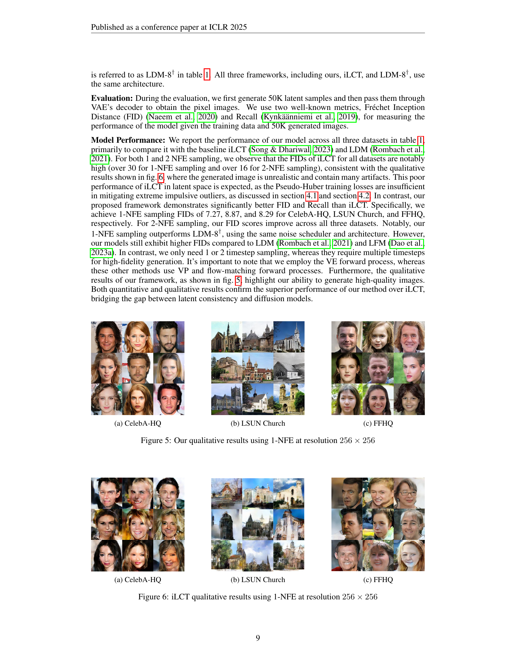
🔼 This figure showcases the qualitative results obtained from the proposed model. Specifically, it presents sample images generated using only one forward diffusion step (1-NFE) at a resolution of 256x256 pixels. The images are visually compared across three different datasets: CelebA-HQ (faces), LSUN Church (church exteriors), and FFHQ (high-resolution faces). This provides a visual demonstration of the model’s ability to generate high-quality images with a minimal number of diffusion steps. The improved image quality reflects the model’s effectiveness and efficiency.
read the caption
Figure 5: Our qualitative results using 1-NFE at resolution 256×256256256256\times 256256 × 256

🔼 This figure shows a qualitative comparison of images generated by the proposed model and the baseline model. The subfigure (a) displays images generated for the CelebA-HQ dataset. The figure demonstrates the improved quality of images generated by the proposed model compared to the baseline. This highlights the effectiveness of the proposed training techniques.
read the caption
(a) CelebA-HQ

🔼 The figure shows the qualitative results of the proposed method on the LSUN Church dataset. The images demonstrate the model’s ability to generate realistic and high-quality images of church scenes, showcasing architectural details and overall scene composition.
read the caption
(b) LSUN Church

🔼 This figure displays the quantitative results obtained by the proposed training technique on the FFHQ dataset. It presents key metrics like FID (Fréchet Inception Distance) and Recall, along with the number of function evaluations (NFE), to evaluate the quality of generated images. The table likely includes comparisons to other state-of-the-art models on the same dataset.
read the caption
(c) FFHQ

🔼 This figure displays the qualitative results obtained from the iLCT model (Improved Latent Consistency Training) when generating images with only one forward diffusion step (1-NFE). The images are generated at a resolution of 256x256 pixels. The purpose is to showcase the quality of images produced by the iLCT model in comparison to other models, highlighting its strengths and weaknesses in terms of image generation quality and diversity.
read the caption
Figure 6: iLCT qualitative results using 1-NFE at resolution 256×256256256256\times 256256 × 256

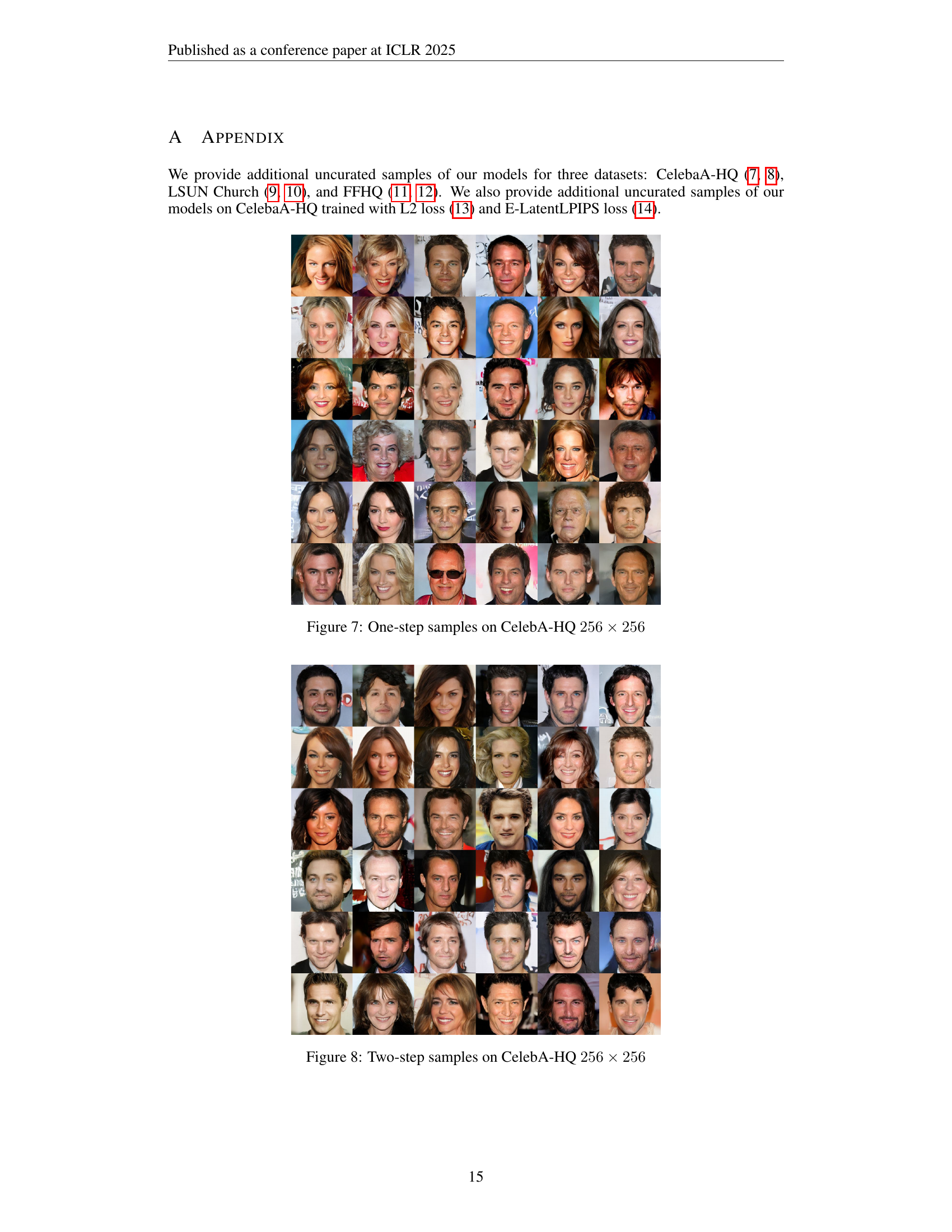
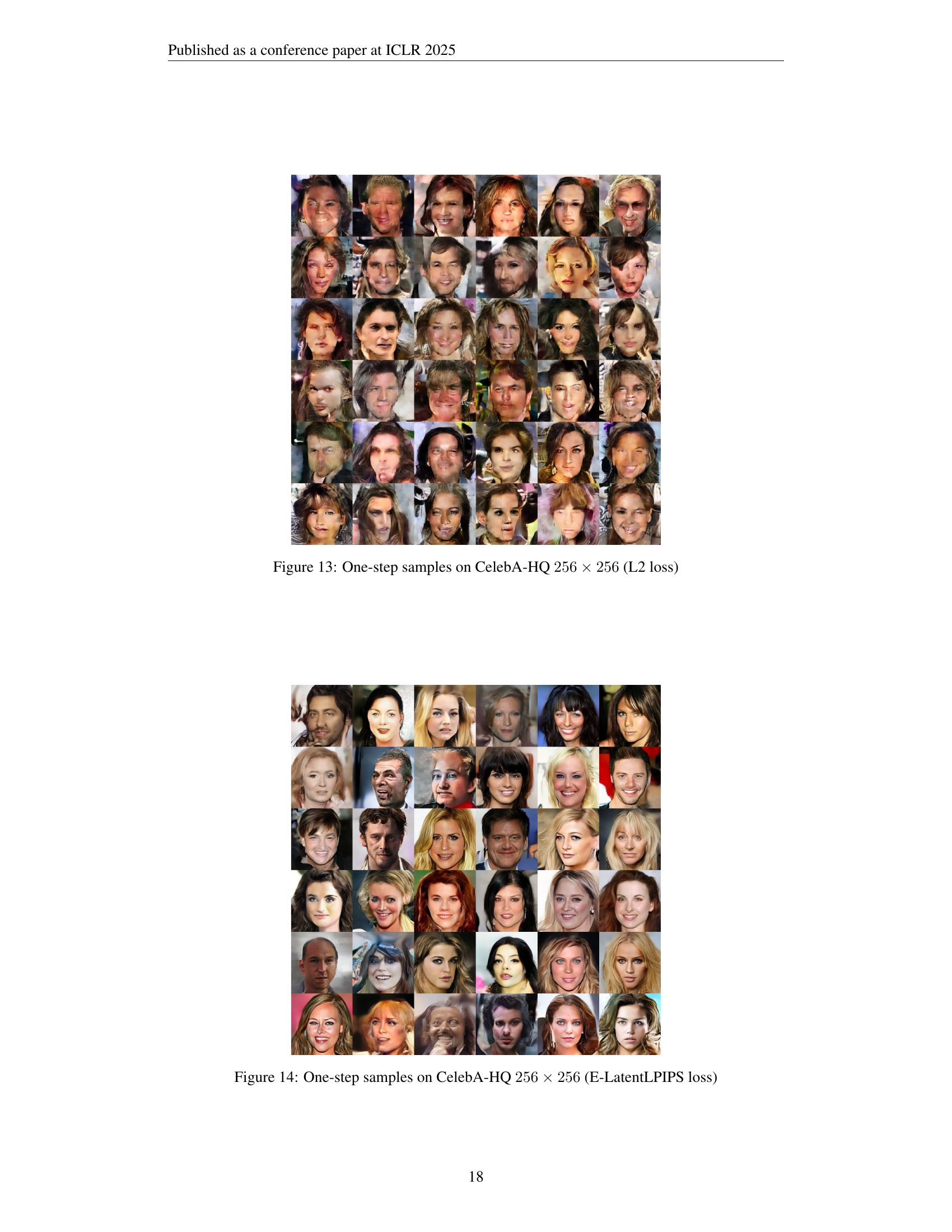
🔼 This figure displays a grid of images generated using the improved latent consistency training technique. Each image is a sample produced in a single step (one-step sampling) and represents the model’s output after applying the proposed training enhancements. The dataset used to train the model is CelebA-HQ, and the generated images are 256x256 pixels in resolution. This visual showcases the quality and diversity of the generated images, demonstrating the effectiveness of the improved technique.
read the caption
Figure 7: One-step samples on CelebA-HQ 256×256256256256\times 256256 × 256

🔼 This figure displays the results of generating images using a latent consistency model with two sampling steps. The images are of size 256x256 pixels and belong to the CelebA-HQ dataset, which is known for its high-quality celebrity face images. The figure demonstrates the model’s ability to generate diverse and realistic-looking faces after undergoing a two-step sampling process, highlighting the quality and detail achievable with the proposed method.
read the caption
Figure 8: Two-step samples on CelebA-HQ 256×256256256256\times 256256 × 256

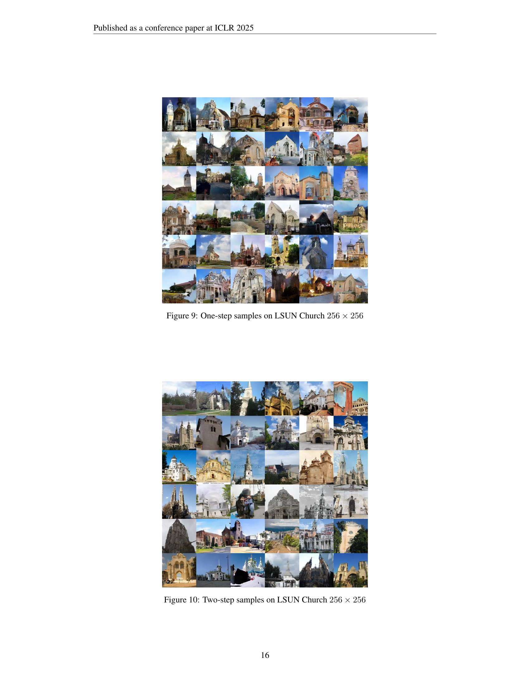
🔼 This figure displays a grid of images generated by a one-step sampling method on the LSUN Church dataset. The images are 256x256 pixels. The figure serves as a qualitative evaluation of the model’s ability to generate realistic and diverse images of church scenes. It is intended to visually demonstrate the quality of the generated images.
read the caption
Figure 9: One-step samples on LSUN Church 256×256256256256\times 256256 × 256

🔼 This figure displays images generated using a latent consistency model trained with the improved techniques presented in the paper. Specifically, it showcases the results of a two-step sampling process on the LSUN Church dataset. Each image in the grid is an example of a generated church scene, demonstrating the model’s ability to generate detailed and varied church architecture. The resolution of each generated image is 256x256 pixels.
read the caption
Figure 10: Two-step samples on LSUN Church 256×256256256256\times 256256 × 256

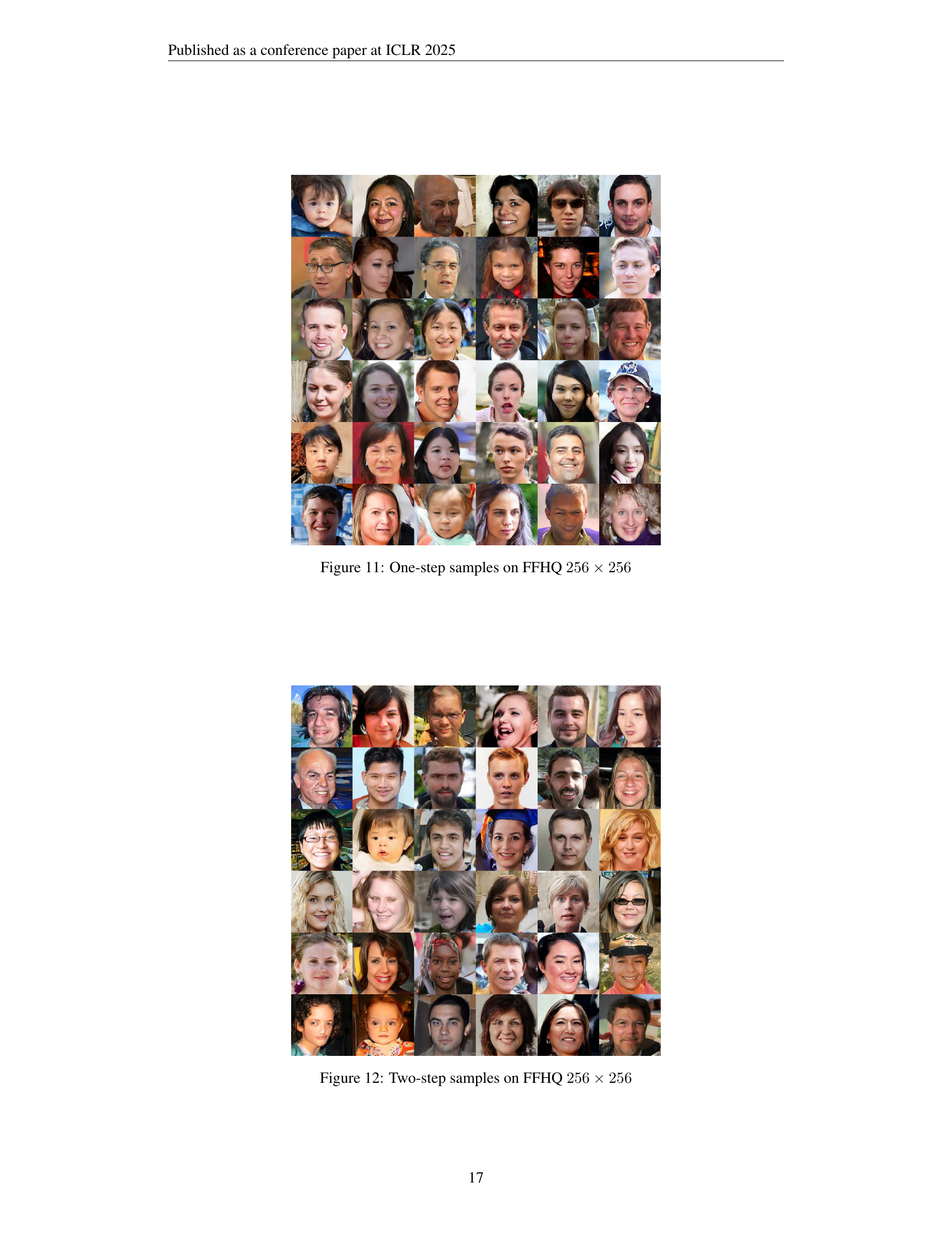
🔼 This figure displays the results of generating images using a one-step sampling method on the FFHQ dataset with a resolution of 256x256 pixels. The images represent a selection of generated samples and showcase the model’s ability to produce realistic-looking high-resolution images of faces. The quality and diversity of the generated images are indicative of the model’s performance.
read the caption
Figure 11: One-step samples on FFHQ 256×256256256256\times 256256 × 256
Full paper#