TL;DR#
Large language models (LLMs) are powerful but opaque. Understanding how semantic information is processed within them is crucial for enhancing their interpretability and control. Existing methods often struggle with the complexity of multi-layer interactions, limiting our ability to analyze and influence feature development. This research tackles this issue by focusing on the dynamics of features across multiple layers.
The proposed approach utilizes sparse autoencoders (SAEs) to track features across different layers of the LLM, creating “flow graphs.” These graphs visually represent how features originate, evolve, and eventually disappear. The researchers demonstrate how manipulating these features through the flow graphs allows for direct and targeted control over the LLM’s output, such as amplifying or suppressing specific themes in text generation. This technique significantly improves our capacity to understand and control LLMs’ behavior.
Key Takeaways#
Why does it matter?#
This paper is crucial because it introduces a novel data-free approach to understand and manipulate the inner workings of large language models (LLMs). This is a significant step towards making LLMs more interpretable, controllable, and reliable, which addresses a key challenge in the field and opens doors for safer and more effective AI systems. The proposed methods offer unique insights into feature evolution, enabling more precise control over model behavior and facilitating the discovery of computational circuits. This will be highly impactful for researchers aiming to improve model transparency and address issues like bias and toxicity.
Visual Insights#

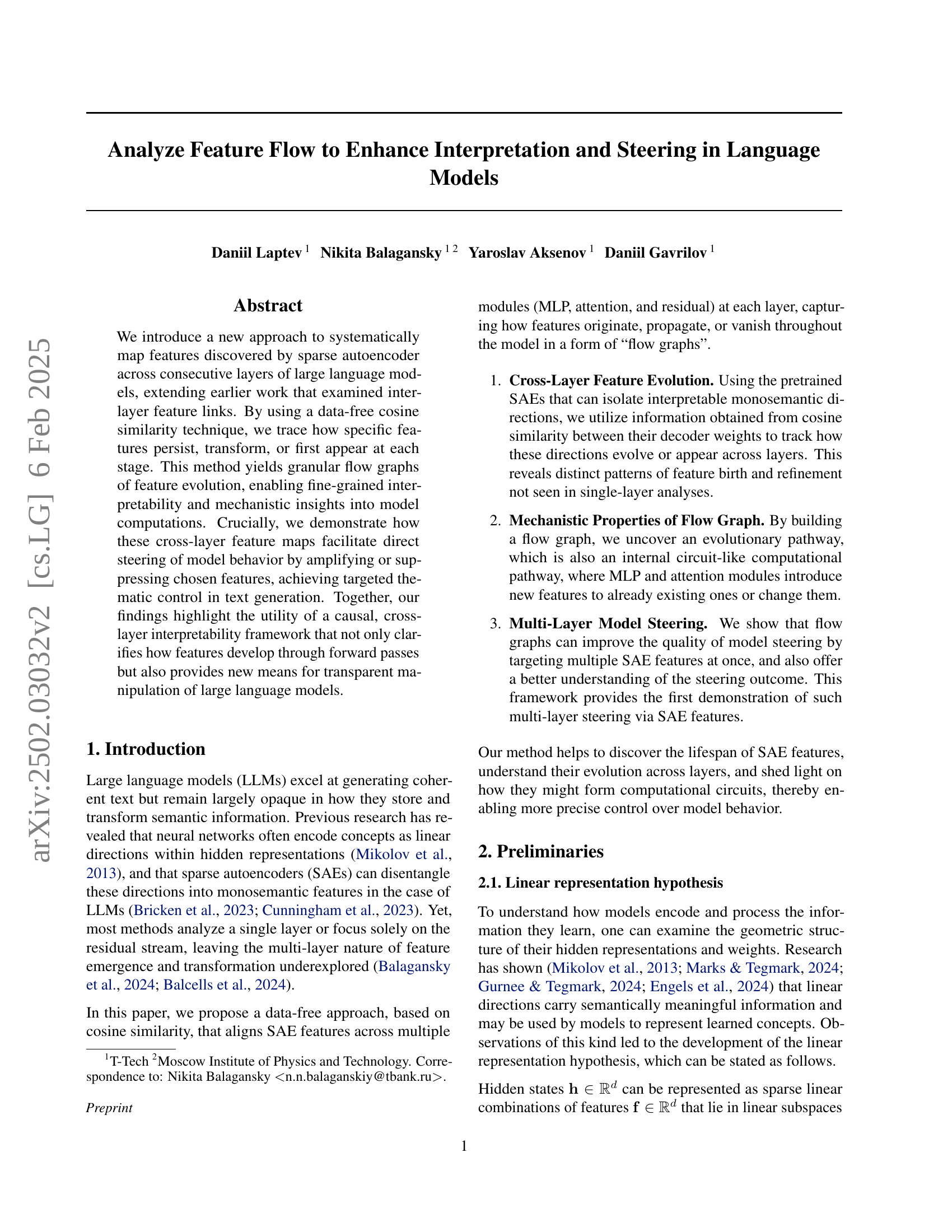
🔼 This figure illustrates the method for inner-layer feature matching. It shows how a feature (represented by its embedding vector) from one layer of a language model is compared to features from other layers and modules (MLP, Attention, Residual Stream) using cosine similarity to find its source. The figure shows that features are identified on the layer outputs, and each feature embedding is compared against all feature embeddings in the MLP and attention blocks of that layer, and also against features from the previous layer’s residual stream. The comparisons determine which modules and preceding layers most influenced the identified feature.
read the caption
Figure 1: Schematic illustration of inner-layer matching. We select a feature with index i𝑖iitalic_i on the SAE trained at the layer output. Its embedding 𝐟𝐟\mathbf{f}bold_f, which is the i𝑖iitalic_ith column of this SAE’s decoder weight, is compared to every column of other SAEs on the same layer (after the MLP and attention blocks, as well as with the SAE on the residual stream before some layer). These comparisons indicate the feature’s source. See Section 3.3 for more details.
| Feature index | Interpretation from Neuronpedia |
|---|---|
| 3/res/9811 | terms related to gravity and its influences |
| 18/res/14053 | terms related to theoretical frameworks and conceptual models |
| 18/res/1336 | references to Dark Matter and astronomical phenomena |
| 20/res/4506 | terms related to physical laws and scientific principles |
| 21/res/13226 | references to quantum concepts and theories |
| 22/res/9002 | terms related to models and their specifications, |
| 22/res/15105 | terms related to force and energy dynamics |
| 23/res/4086 | terms related to forces and dynamics in physical systems |
| 24/res/7017 | terms related to electromagnetic interactions and properties |
| 24/res/14548 | terms and references related to particle physics and standard model parameters |
🔼 This table lists the features initially selected for the deactivation experiment targeting the theme of ‘Scientific concepts and entities’. Each row represents a feature, identified by its layer, module (residual, MLP, or attention), and index within that module. The ‘Interpretation’ column provides a brief description of the semantic meaning of each feature according to the Neuronpedia, a tool for interpreting neural network activations. These features were chosen as they were associated with the ‘Scientific concepts and entities’ theme according to Neuronpedia. The experiment involved deactivating these features in order to investigate their effect on the model’s text generation, helping to understand causal relations between model features and their semantic effect.
read the caption
Table 1: Features initially chosen for deactivation of “Scientific concepts and entities” theme.
In-depth insights#
Cross-Layer Feature Flow#
The concept of ‘Cross-Layer Feature Flow’ in the context of analyzing large language models (LLMs) offers a powerful approach to understanding how features evolve and interact throughout the network’s layers. It moves beyond the limitations of single-layer analysis by tracking the lifespan of features, revealing how they originate, transform, and even vanish as they propagate through different modules like MLPs and attention mechanisms. This cross-layer perspective provides crucial mechanistic insights, revealing not only how features develop but also highlighting the formation of computational circuits, pathways where features influence each other across layers. The ability to map feature evolution using a data-free technique like cosine similarity between sparse autoencoder (SAE) features, greatly enhances interpretability. Furthermore, understanding the flow graph opens the door to direct model steering, enabling targeted thematic control by amplifying or suppressing specific features across multiple layers. This facilitates more precise, transparent manipulation of LLMs, leading to improved control over the model’s behavior and increased understanding of its inner workings. Overall, the study of Cross-Layer Feature Flow offers a significant advance in causal interpretability and control of LLMs.
Multi-Layer Steering#
The concept of “Multi-Layer Steering” in the context of large language models (LLMs) presents a significant advancement in controlling model behavior. Instead of manipulating features within a single layer, this approach leverages a causal, cross-layer interpretability framework to trace the evolution of features across multiple layers. This allows for more precise control by either amplifying or suppressing specific features, enabling targeted thematic control in text generation. By identifying interconnected features across layers, this approach provides a better understanding of how model computations unfold and enhances the effectiveness of steering interventions. Multi-layer steering is superior to single-layer steering as it accounts for the complex interplay between features and their propagation across the neural network’s depth. Furthermore, it offers the potential for discovering computational circuits, identifying interconnected pathways in the model. This framework moves beyond simple feature manipulation to provide a more nuanced and effective means to guide the model’s behavior, making LLMs significantly more transparent and controllable.
SAE Feature Matching#
SAE (Sparse Autoencoder) feature matching is a crucial technique for analyzing the flow of interpretable features across layers in large language models. It leverages the sparse representations learned by SAEs to identify corresponding features across different layers and modules, thus revealing how these features evolve and interact throughout the model’s computation. The core idea is to use a similarity metric (e.g., cosine similarity) between the decoder weights of SAEs trained at different layers to find matching features. This allows for the construction of cross-layer feature flow graphs that provide insights into the model’s internal mechanisms. This approach is data-free, meaning it doesn’t require any additional training data beyond what was used to train the original model and SAEs, making it computationally efficient. Effective SAE feature matching is vital for enhancing model interpretability, enabling a deeper understanding of model behavior, and facilitating targeted model steering. Challenges in this process may involve choosing appropriate similarity metrics, handling feature sparsity, and addressing potentially noisy matches due to model complexity. The success of SAE feature matching hinges upon the quality of the trained SAEs; the degree of feature disentanglement impacts the clarity and reliability of identified matches.
Linear Feature Circuits#
The concept of “Linear Feature Circuits” in large language models (LLMs) suggests that model computations can be decomposed into smaller, interconnected subnetworks. These circuits, characterized by linear transformations of features, represent specific operations or semantic processing steps. Understanding these circuits is crucial for enhancing interpretability, as it allows us to trace the flow of information and how features evolve throughout the model’s layers. Identifying linear feature circuits can also greatly improve model steering, providing more granular control over LLM output. This method would allow researchers to modify the behavior of the model by selectively activating or suppressing specific features within these circuits. Further research into this area would reveal potential mechanistic insights into how LLMs process information, leading to advancements in the development of more efficient, controllable, and interpretable AI systems.
Model Interpretability#
Model interpretability is a crucial aspect of research, particularly in the context of large language models (LLMs). Understanding how LLMs arrive at their outputs is vital for building trust, identifying biases, and improving model performance. This research explores interpretability by mapping features through the model’s layers using sparse autoencoders (SAEs). SAEs help isolate interpretable features, allowing researchers to trace their evolution across multiple layers and various model components (MLP, attention). This cross-layer analysis reveals how features originate, transform, or disappear, providing fine-grained insights into internal computations. The research goes beyond simple analysis, demonstrating how understanding feature flow enables direct model steering by amplifying or suppressing specific features to achieve targeted thematic control in text generation. This demonstrates a strong connection between interpretability and controllability of LLMs. The data-free approach used, relying on cosine similarity between SAE decoder weights, makes the analysis scalable and widely applicable. Overall, the findings highlight the importance of a causal, multi-layer interpretability framework for both understanding and controlling LLMs. The creation of flow graphs offers a novel way to visualize this feature evolution, opening new avenues for research and development of more explainable and controllable AI systems.
More visual insights#
More on figures

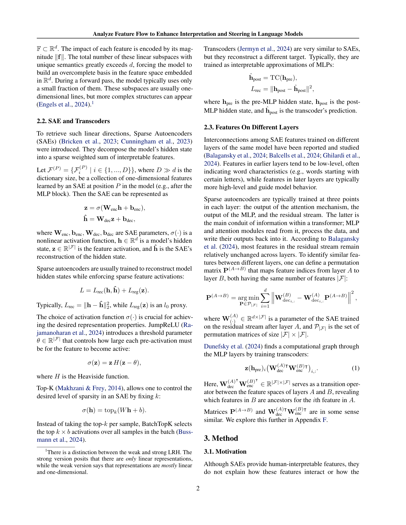
🔼 This figure shows a flow graph that visualizes how a specific feature (index 14548) in the 24th residual layer of a large language model evolves across different layers and modules. The graph illustrates the feature’s origin, its propagation through the model’s architecture (MLP, attention, residual streams), and how it transforms or interacts with other features. Nodes represent features identified by sparse autoencoders (SAEs), and edges indicate relationships between features across layers. This visualization is used in the deactivation experiments (Section 5.2) to understand the causal relationships between features and their effect on downstream model behavior. More details are provided in Appendix E.
read the caption
Figure 2: An illustration of the resulting flow graph, which we also use in the deactivation experiment (section 5.2). As a starting point, we select the feature on the 24th-layer residual with index 14548. For a detailed explanation of this graph, see Appendix E.
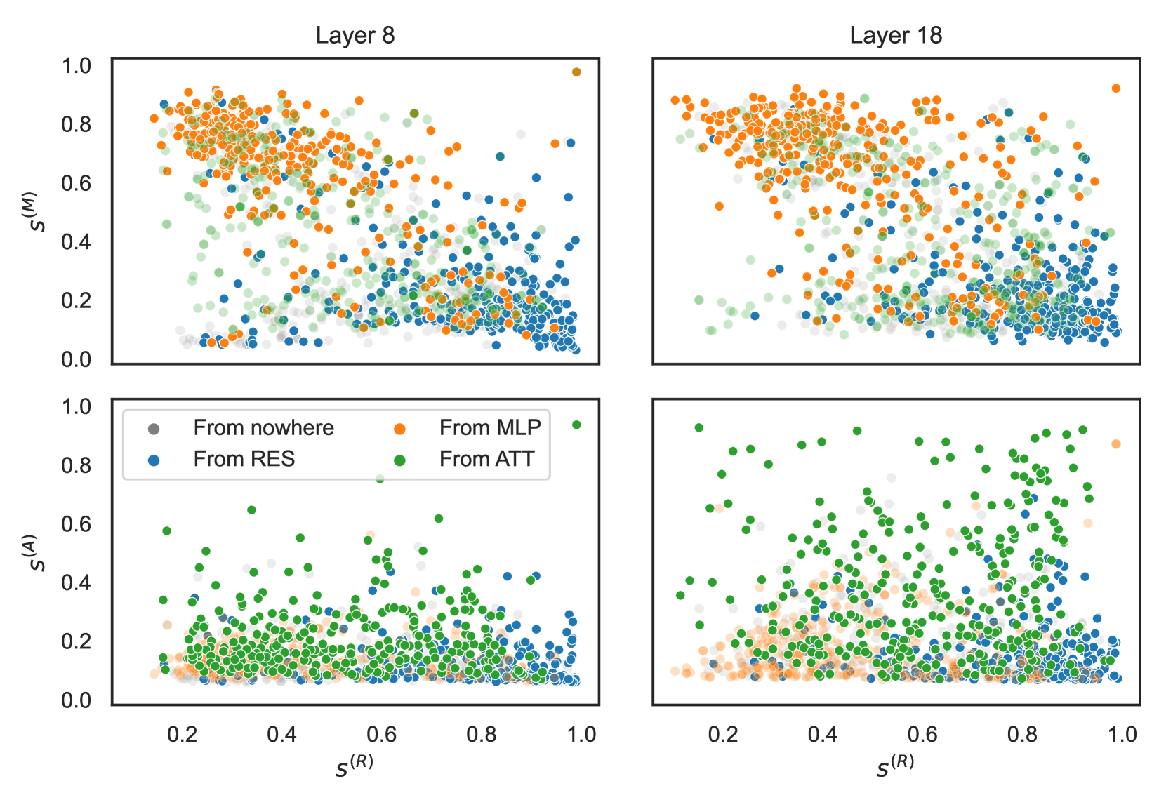
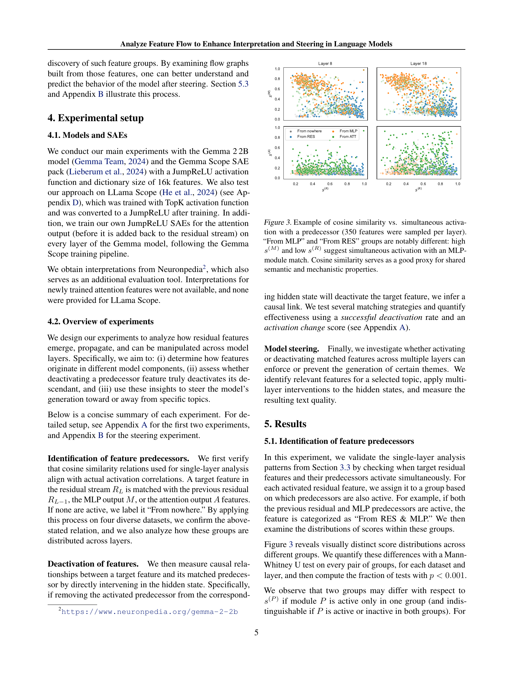
🔼 This figure displays the results of an experiment comparing cosine similarity between a target feature and its predecessors (features from the previous layer, MLP, and attention modules) with their simultaneous activation. The data shows distinct patterns of simultaneous activation for different groups of features. Specifically, features grouped as ‘From MLP’ show high similarity to MLP predecessors and low similarity to residual stream predecessors, indicating that these features are primarily processed by the MLP module. In contrast, features in the ‘From RES’ group exhibit the opposite pattern, suggesting that these features originate from and are primarily propagated through the residual stream. This analysis demonstrates that cosine similarity between a feature and its predecessors serves as a strong indicator of their relationship (i.e., shared semantic and mechanistic properties). The experiment involved sampling 350 features per layer, highlighting the large-scale nature of the analysis and its relevance to understanding the complex computational behavior within a large language model.
read the caption
Figure 3: Example of cosine similarity vs. simultaneous activation with a predecessor (350 features were sampled per layer). “From MLP” and “From RES” groups are notably different: high s(M)superscript𝑠𝑀s^{(M)}italic_s start_POSTSUPERSCRIPT ( italic_M ) end_POSTSUPERSCRIPT and low s(R)superscript𝑠𝑅s^{(R)}italic_s start_POSTSUPERSCRIPT ( italic_R ) end_POSTSUPERSCRIPT suggest simultaneous activation with an MLP-module match. Cosine similarity serves as a good proxy for shared semantic and mechanistic properties.

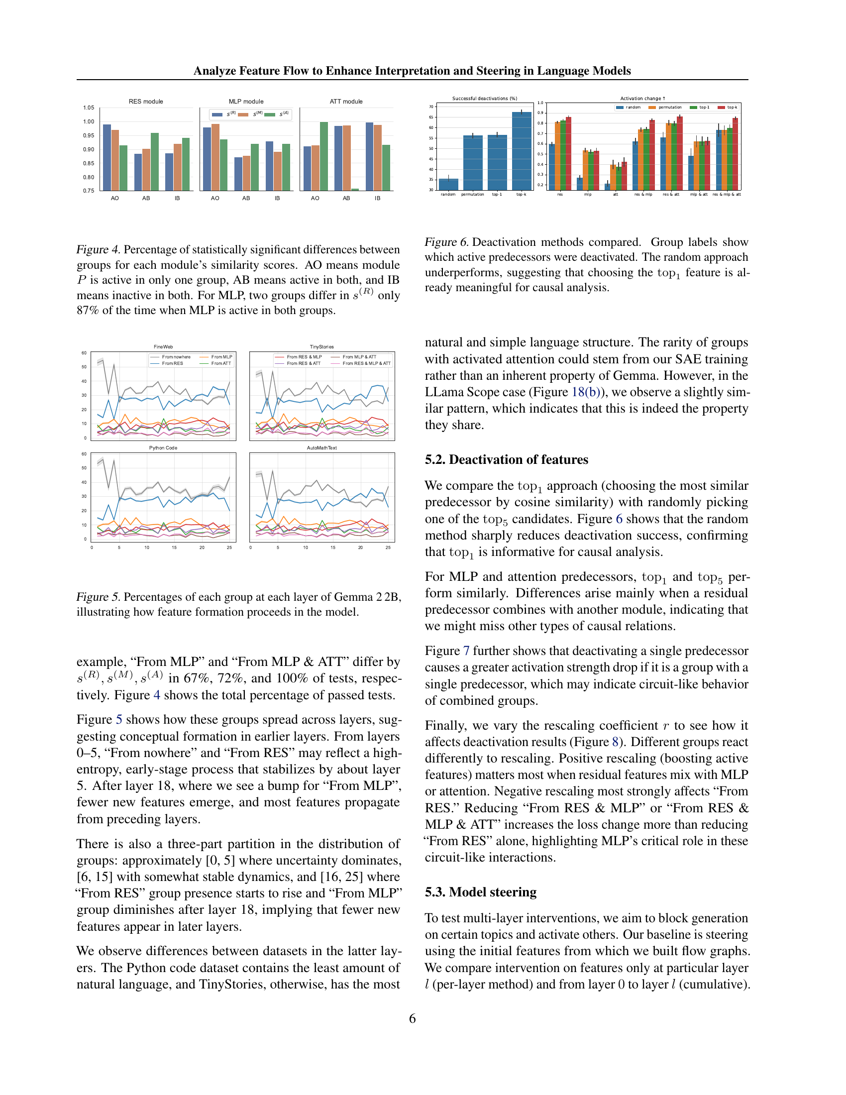
🔼 This figure displays the results of a statistical analysis comparing the similarity scores of different groups of features based on their activation patterns in different modules (MLP, Attention, Residual) of a transformer layer. The analysis determines whether the similarity scores between feature groups are statistically significantly different. The groups are categorized by whether a specific module is active (A) or inactive (I) in both groups (AB, IB) or only one group (AO). The figure visualizes the percentage of statistically significant differences (p<0.001) for each module, revealing the relationships between feature activation and similarity scores. For instance, it shows that for MLP, there is an 87% probability that two feature groups will have statistically different s(R) scores when MLP is active in both groups.
read the caption
Figure 4: Percentage of statistically significant differences between groups for each module’s similarity scores. AO means module P𝑃Pitalic_P is active in only one group, AB means active in both, and IB means inactive in both. For MLP, two groups differ in s(R)superscript𝑠𝑅s^{(R)}italic_s start_POSTSUPERSCRIPT ( italic_R ) end_POSTSUPERSCRIPT only 87% of the time when MLP is active in both groups.

🔼 This figure visualizes the distribution of feature groups across different layers of the Gemma 2-2B language model. Each group represents how features originate: from a previous layer’s residual stream, from the MLP (Multi-Layer Perceptron) module, from the attention module, or from a combination of these sources. The percentages in the chart illustrate the proportion of features in each category at each layer. This provides insights into the dynamic process of feature emergence and transformation as information flows through the model’s layers.
read the caption
Figure 5: Percentages of each group at each layer of Gemma 2 2B, illustrating how feature formation proceeds in the model.

🔼 This figure compares different methods for deactivating features in a language model to analyze causal relationships. The x-axis represents different groups of features, categorized by which predecessor features were deactivated before evaluating the impact on the target feature. The y-axis shows the percentage of successful deactivations for each group. The ‘random’ approach serves as a baseline, randomly choosing a predecessor to deactivate. The other methods, such as ’top-1’, select the most similar predecessor based on cosine similarity. The results demonstrate that the ’top-1’ method significantly outperforms the ‘random’ method, suggesting that selecting the most similar predecessor is a more effective strategy for revealing causal links between features.
read the caption
Figure 6: Deactivation methods compared. Group labels show which active predecessors were deactivated. The random approach underperforms, suggesting that choosing the top1subscripttop1\operatorname{top}_{1}roman_top start_POSTSUBSCRIPT 1 end_POSTSUBSCRIPT feature is already meaningful for causal analysis.

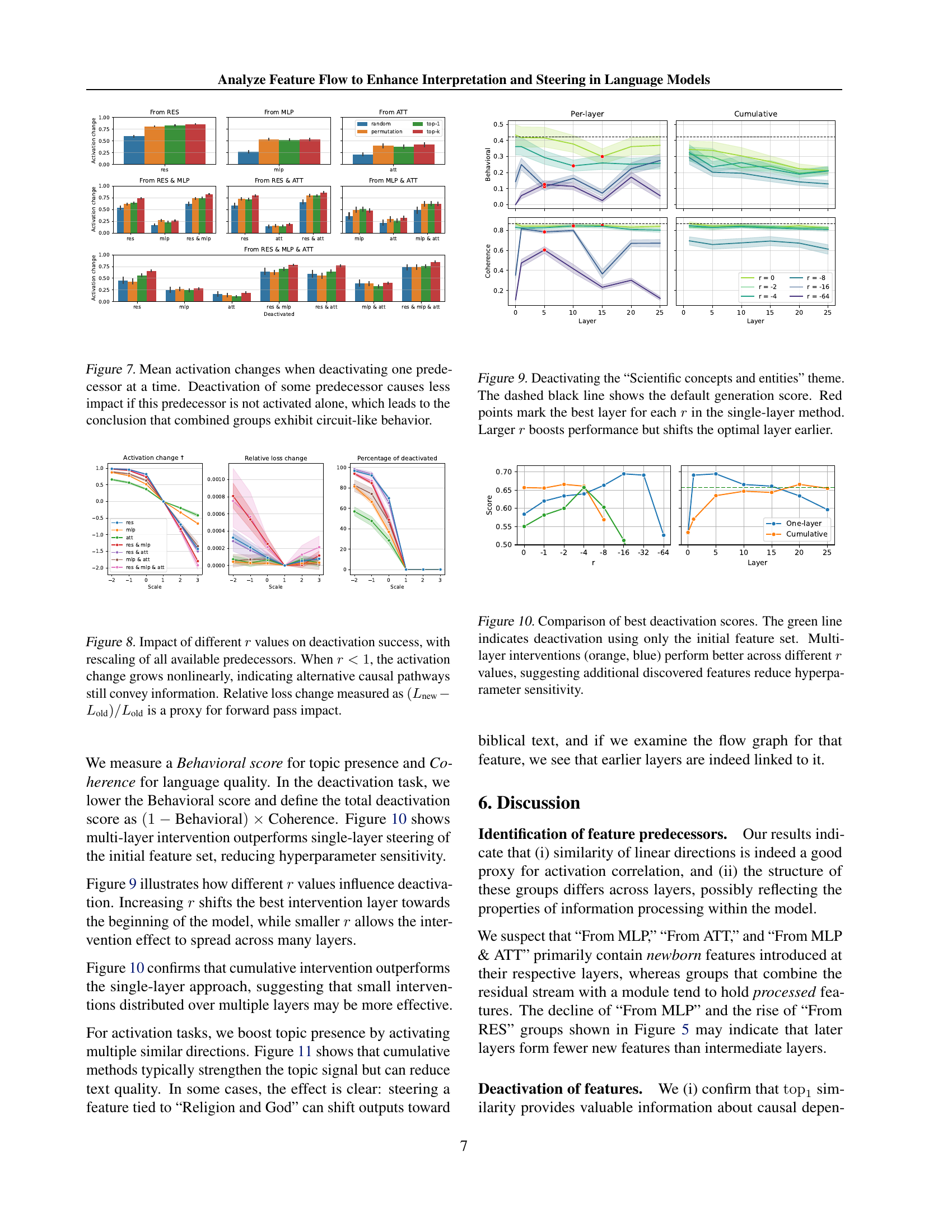
🔼 This figure displays the average changes in activation strength for target features when one of their predecessor features is deactivated. The results show that deactivating a single predecessor feature has a more significant impact when that predecessor feature is the only active one. When multiple predecessor features are simultaneously activated, deactivating one of them has a smaller impact on the target feature. This suggests that multiple predecessor features might be part of a larger circuit, such that deactivating just one does not disrupt the overall circuit functionality. The findings indicate that the model’s behavior is not solely dependent on single features, but rather groups of features working together in interconnected ways.
read the caption
Figure 7: Mean activation changes when deactivating one predecessor at a time. Deactivation of some predecessor causes less impact if this predecessor is not activated alone, which leads to the conclusion that combined groups exhibit circuit-like behavior.

🔼 Figure 8 illustrates the impact of the rescaling coefficient (r) on the success rate of deactivating features in a language model. The x-axis represents different values of r, while the y-axis shows the resulting activation change. When r is less than 1 (meaning the features are being suppressed), the activation change demonstrates nonlinear growth. This nonlinearity suggests that even when a direct causal predecessor is deactivated, alternative pathways might still allow the feature to remain active, thus conveying information. The graph also displays the relative loss change, which is calculated as (Lnew - Lold) / Lold and serves as a proxy to assess the impact on the model’s forward pass during the deactivation process.
read the caption
Figure 8: Impact of different r𝑟ritalic_r values on deactivation success, with rescaling of all available predecessors. When r<1𝑟1r<1italic_r < 1, the activation change grows nonlinearly, indicating alternative causal pathways still convey information. Relative loss change measured as (Lnew−Lold)/Loldsubscript𝐿newsubscript𝐿oldsubscript𝐿old(L_{\text{new}}-L_{\text{old}})/L_{\text{old}}( italic_L start_POSTSUBSCRIPT new end_POSTSUBSCRIPT - italic_L start_POSTSUBSCRIPT old end_POSTSUBSCRIPT ) / italic_L start_POSTSUBSCRIPT old end_POSTSUBSCRIPT is a proxy for forward pass impact.

🔼 Figure 9 illustrates an experiment on deactivating the ‘Scientific concepts and entities’ theme in text generation. The graph displays the impact of different rescaling coefficients (r) applied at various layers of a language model on both the coherence and presence of the target theme in generated text. The dashed black line represents the baseline generation quality without any intervention. Red data points highlight the layer where the deactivation strategy achieves the best results for each value of r. The results show that increasing the rescaling coefficient (r) improves the effectiveness of theme suppression, although the optimal layer for intervention shifts to earlier layers as r increases.
read the caption
Figure 9: Deactivating the “Scientific concepts and entities” theme. The dashed black line shows the default generation score. Red points mark the best layer for each r𝑟ritalic_r in the single-layer method. Larger r𝑟ritalic_r boosts performance but shifts the optimal layer earlier.

🔼 Figure 10 displays the results of an experiment comparing different model steering strategies. The goal was to deactivate a specific theme in text generation. The green line represents a baseline where only the initially identified features related to the theme were deactivated. The orange and blue lines show the results when multiple layers of features were targeted for deactivation (multi-layer interventions). The x-axis likely represents different layers of the model and the y-axis likely shows a performance metric (a combination of metrics that capture the balance between successfully removing the unwanted theme and maintaining text quality). Across different values of the hyperparameter r (presumably controlling the strength of the deactivation), the multi-layer strategies consistently outperformed the single-layer strategy. This suggests that including additional, related features discovered via the flow graph analysis improves the robustness and effectiveness of the deactivation process, reducing sensitivity to the specific value of the hyperparameter.
read the caption
Figure 10: Comparison of best deactivation scores. The green line indicates deactivation using only the initial feature set. Multi-layer interventions (orange, blue) perform better across different r𝑟ritalic_r values, suggesting additional discovered features reduce hyperparameter sensitivity.

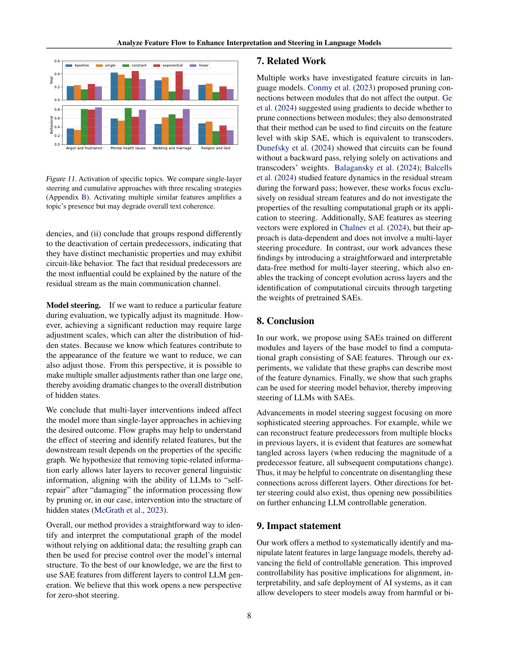
🔼 This figure displays the results of an experiment on activating specific topics in text generation using a language model. Three different rescaling strategies (detailed in Appendix B) were applied to both single-layer and cumulative steering approaches. The results show that activating multiple similar features effectively amplifies the presence of the target topic in the generated text. However, this improvement in topic presence sometimes comes at the cost of reduced text coherence, indicating a trade-off between targeted topic emphasis and overall text quality.
read the caption
Figure 11: Activation of specific topics. We compare single-layer steering and cumulative approaches with three rescaling strategies (Appendix B). Activating multiple similar features amplifies a topic’s presence but may degrade overall text coherence.

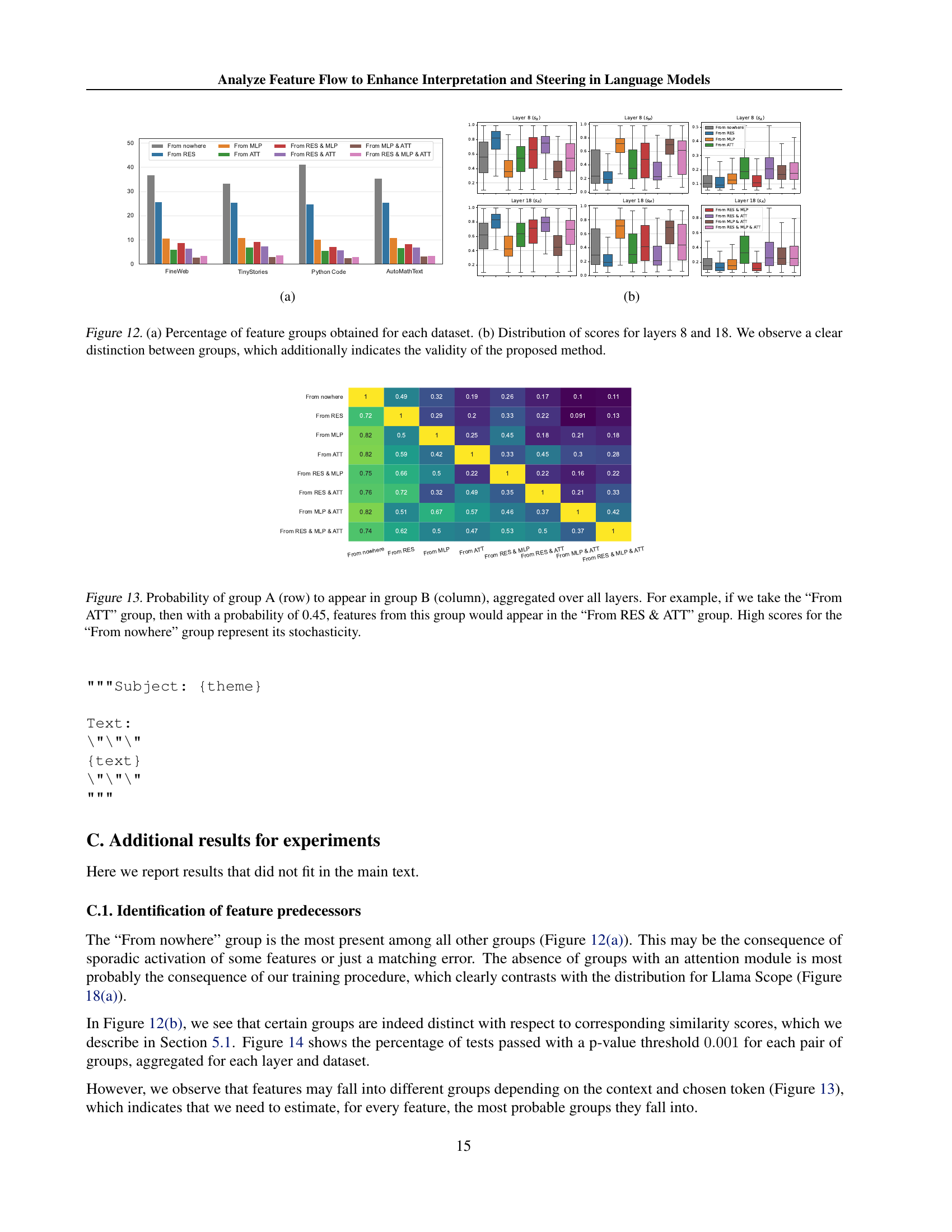
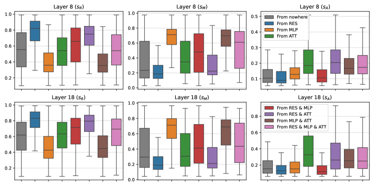
🔼 Figure 12 presents a detailed analysis of feature group distribution and score distribution across different layers of a language model. Part (a) shows the percentage of features falling into each of the eight identified groups (based on their predecessor activations) for four different datasets: FineWeb, TinyStories, Python Code, and AutoMathText. This visualization helps to understand how the origin and development of features vary depending on dataset characteristics. Part (b) provides a comparative analysis of score distributions for layers 8 and 18 across these feature groups, showing the distinct patterns of score distribution for each group. The clear separation between these distributions visually validates the proposed approach for identifying feature origins and tracking their evolution across layers.
read the caption
Figure 12: (a) Percentage of feature groups obtained for each dataset. (b) Distribution of scores for layers 8 and 18. We observe a clear distinction between groups, which additionally indicates the validity of the proposed method.
🔼 This figure shows a matrix representing the probability of features originating from a specific group (e.g., ‘From ATT’, ‘From RES’, etc.) at one layer, to subsequently appear in another group at a later layer. Each cell (i,j) in the matrix shows the probability of a feature belonging to group ‘i’ at some layer appearing in group ‘j’ at a later layer in the model’s processing. The rows represent the starting group, while the columns represent the resulting group after propagating through multiple layers. A high value indicates a strong likelihood of transition from the source group to the target group. The high probabilities on the diagonal reflect features that persist through layers. The ‘From Nowhere’ group represents features that appear without a clear preceding origin.
read the caption
Figure 13: Probability of group A (row) to appear in group B (column), aggregated over all layers. For example, if we take the “From ATT” group, then with a probability of 0.45, features from this group would appear in the “From RES & ATT” group. High scores for the “From nowhere” group represent its stochasticity.

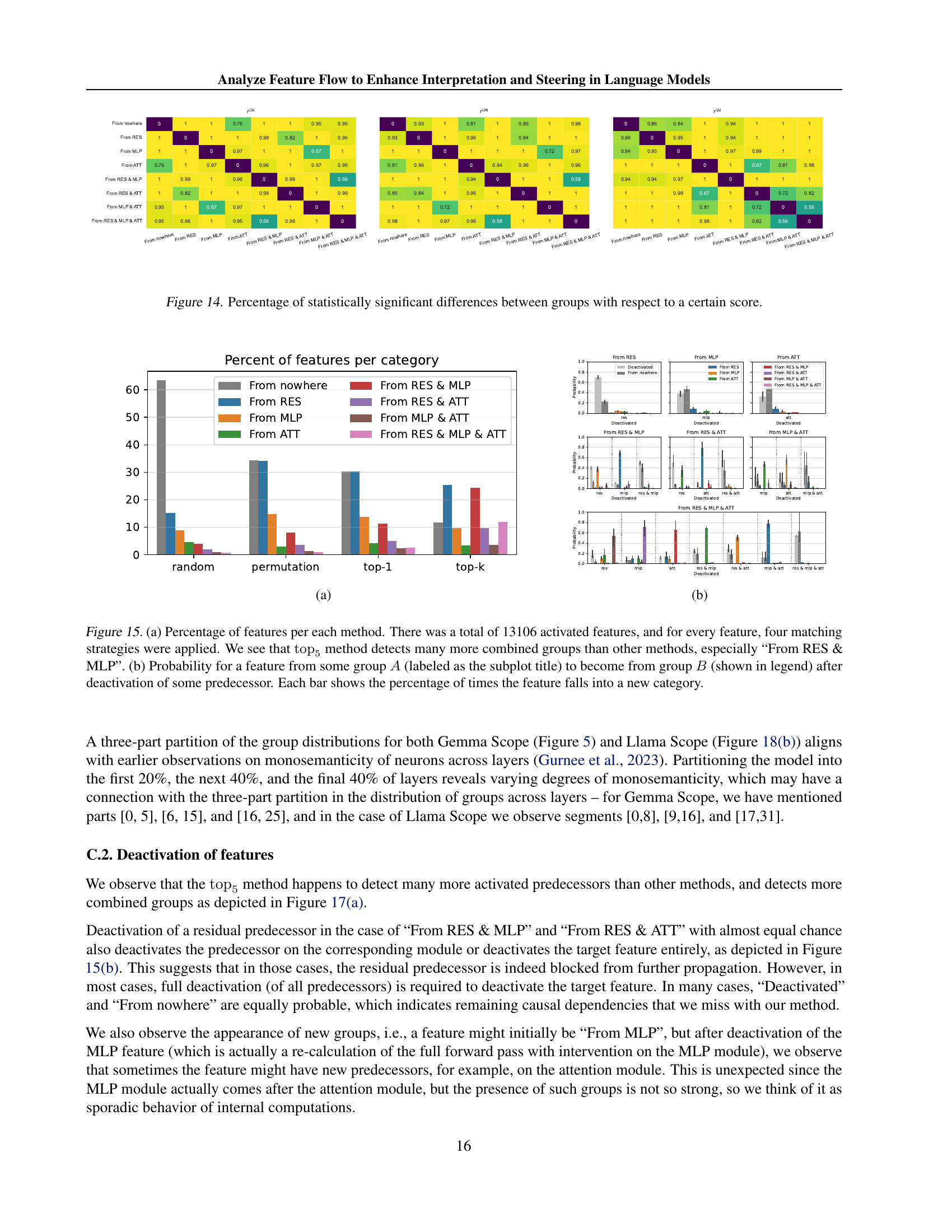
🔼 This figure displays the results of Mann-Whitney U tests comparing the distributions of similarity scores (cosine similarity between decoder weights) across different groups of features. Each group represents a combination of activated predecessor features (from the previous layer, MLP, or attention). The figure shows the percentage of tests that yielded statistically significant results (p<0.001) for each pair of groups across different layers and datasets. This visualizes which groups of features exhibit distinct similarity score distributions, suggesting differences in their origins and relationship to predecessors.
read the caption
Figure 14: Percentage of statistically significant differences between groups with respect to a certain score.

🔼 This figure presents a comparison of four different methods for identifying feature predecessors in a language model. Subplot (a) shows the percentage of features assigned to each of the eight possible predecessor groups (e.g., ‘From RES’, ‘From MLP & ATT’) for each of the four matching methods (random, permutation, top1, top5). The top5 method, which considers the top 5 most similar predecessors, identifies significantly more features belonging to combined groups (e.g., ‘From RES & MLP’) than the other methods. Subplot (b) further examines the effects of deactivating a predecessor feature. For each of the eight predecessor groups, it shows the probability of a feature originally belonging to that group transitioning to a different group after deactivation. Each bar represents the percentage of times a feature changes group after deactivation.
read the caption
Figure 15: (a) Percentage of features per each method. There was a total of 13106 activated features, and for every feature, four matching strategies were applied. We see that top5subscripttop5\operatorname{top}_{5}roman_top start_POSTSUBSCRIPT 5 end_POSTSUBSCRIPT method detects many more combined groups than other methods, especially “From RES & MLP”. (b) Probability for a feature from some group A𝐴Aitalic_A (labeled as the subplot title) to become from group B𝐵Bitalic_B (shown in legend) after deactivation of some predecessor. Each bar shows the percentage of times the feature falls into a new category.

🔼 This figure presents the results of a model steering experiment. The researchers selected features from specific layers of a language model’s flow graph, and then applied four different steering strategies to these features. The experiment aimed to determine the optimal layer for intervention to achieve the best results in terms of the model’s ability to generate text aligning with a specific theme. The bar chart displays the best performance attained by each steering strategy across various layers, showing that steering at layers other than layer 12 can sometimes yield better results.
read the caption
Figure 16: From each flow graph, we select features on a particular layer l𝑙litalic_l and perform steering with the four different strategies. Bars represent the best result for each layer among all scores s𝑠sitalic_s. In some cases, steering on a layer other than 12 may improve results.

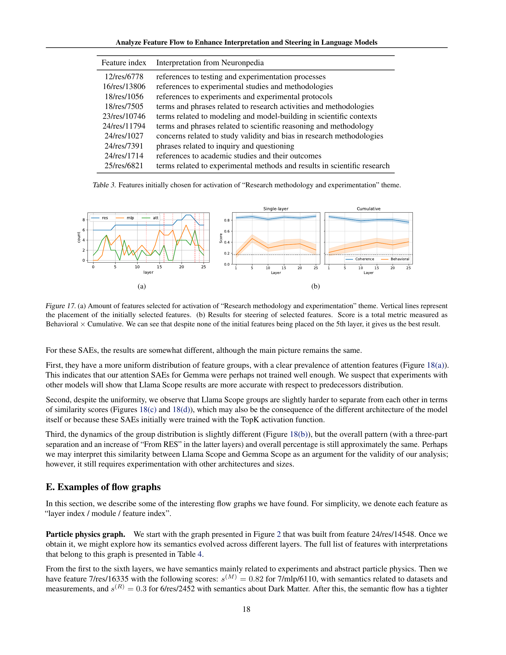
🔼 This figure visualizes the results of an experiment on model steering, focusing on the theme of ‘Research methodology and experimentation’. Part (a) shows the number of features selected for activation across different layers of the model. Vertical lines indicate the initial features selected for this theme. Part (b) presents the results of the model steering process itself, showing the total score achieved (Behavioral score multiplied by Cumulative score) for different steering strategies. The key observation is that while the initial features were not located on layer 5, steering at layer 5 produced the best overall result, suggesting that optimal steering may not always align with the location of initially selected features.
read the caption
Figure 17: (a) Amount of features selected for activation of “Research methodology and experimentation” theme. Vertical lines represent the placement of the initially selected features. (b) Results for steering of selected features. Score is a total metric measured as Behavioral×CumulativeBehavioralCumulative\text{Behavioral}\times\text{Cumulative}Behavioral × Cumulative. We can see that despite none of the initial features being placed on the 5th layer, it gives us the best result.

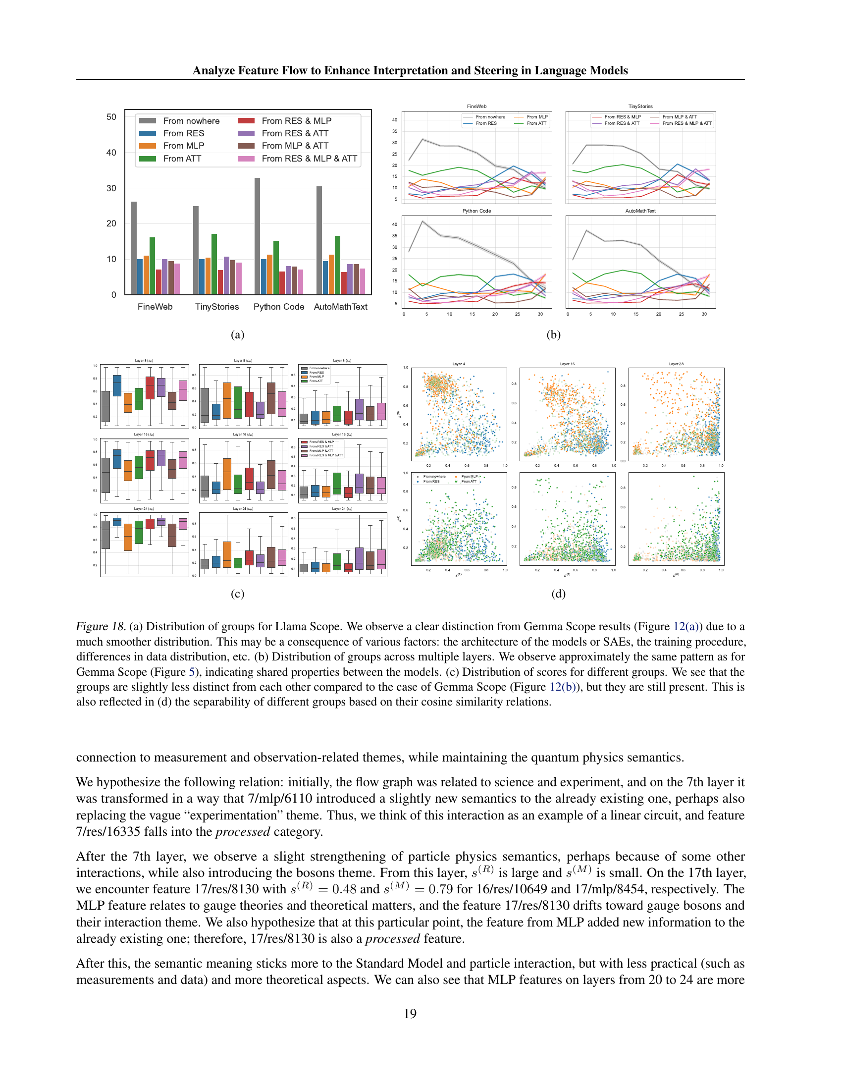
🔼 Figure 18 compares the distribution of feature groups and their cosine similarity scores between LlamaScope and GemmaScope models. Panel (a) shows that LlamaScope has a much smoother distribution of feature groups compared to GemmaScope (Figure 12), likely due to differences in model architecture, SAE training, or data distribution. Panel (b) demonstrates that LlamaScope exhibits a similar layer-wise pattern of feature group distribution to GemmaScope (Figure 5), suggesting shared underlying properties. Panels (c) and (d) further illustrate these similarities and differences, showing that while LlamaScope’s feature groups are less distinct in terms of cosine similarity compared to GemmaScope (Figure 12), the groups are still distinguishable.
read the caption
Figure 18: (a) Distribution of groups for Llama Scope. We observe a clear distinction from Gemma Scope results (Figure 12) due to a much smoother distribution. This may be a consequence of various factors: the architecture of the models or SAEs, the training procedure, differences in data distribution, etc. (b) Distribution of groups across multiple layers. We observe approximately the same pattern as for Gemma Scope (Figure 5), indicating shared properties between the models. (c) Distribution of scores for different groups. We see that the groups are slightly less distinct from each other compared to the case of Gemma Scope (Figure 12), but they are still present. This is also reflected in (d) the separability of different groups based on their cosine similarity relations.

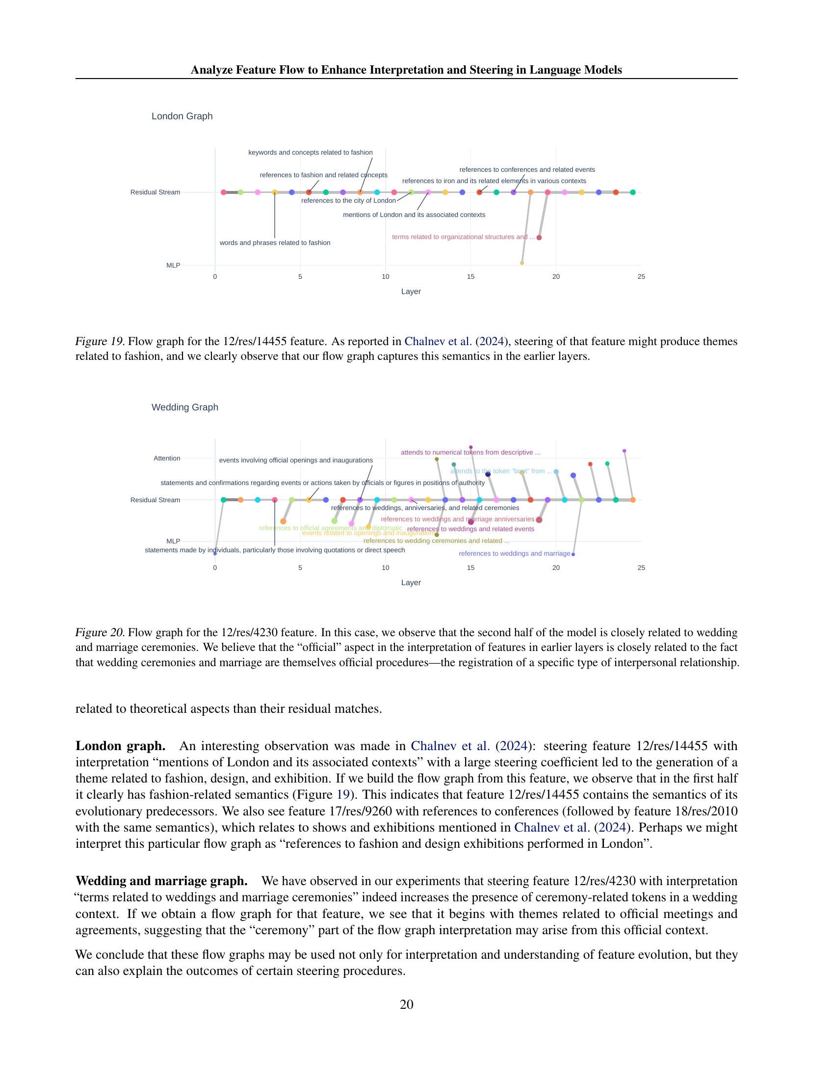
🔼 This figure visualizes the flow graph for feature 12/res/14455. The graph tracks the evolution of this feature across different layers of the language model, showing how its semantic meaning changes. Chalnev et al. (2024) demonstrated that steering this specific feature led to text generation focused on fashion-related themes. This flow graph confirms this, showing a clear presence of fashion-related semantics in the earlier layers of the model. The nodes in the graph represent features identified by Sparse Autoencoders (SAEs), and edges indicate their connections across layers. The colors likely represent different modules within the language model (e.g., attention, MLP, residual streams). The graph illustrates how the feature’s meaning is built upon and transformed through these different model components. Analyzing such a graph allows researchers to better understand the model’s inner workings and improve interpretability and steering.
read the caption
Figure 19: Flow graph for the 12/res/14455 feature. As reported in Chalnev et al. (2024), steering of that feature might produce themes related to fashion, and we clearly observe that our flow graph captures this semantics in the earlier layers.

🔼 This figure visualizes the flow of feature 12/res/4230 through the layers of a language model. The feature is initially related to the official aspects of events and agreements, but in the latter half of the model, its semantic meaning shifts strongly towards wedding and marriage ceremonies. This shift reflects the model’s association of weddings and marriages with official registration processes, a specific type of interpersonal relationship.
read the caption
Figure 20: Flow graph for the 12/res/4230 feature. In this case, we observe that the second half of the model is closely related to wedding and marriage ceremonies. We believe that the “official” aspect in the interpretation of features in earlier layers is closely related to the fact that wedding ceremonies and marriage are themselves official procedures—the registration of a specific type of interpersonal relationship.

🔼 This figure illustrates the concept of using sparse autoencoders (SAEs) to model the transformation of features between consecutive layers in a neural network. Two SAEs, one for layer ’t’ and one for layer ’t+1’, are shown. A learned transition matrix ‘T’ connects the two SAEs, representing the transformation of the feature representations from layer ’t’ to layer ’t+1’. This effectively shows how the SAEs can function as a transcoder, mapping features from one layer to the next, revealing the relationships between features across different layers of the network. This is a key element of their proposed multi-layer interpretability framework.
read the caption
Figure 21: Two SAEs with a learned transition matrix T𝑇Titalic_T can be seen as a transcoder from layer t𝑡titalic_t to layer t+1𝑡1t+1italic_t + 1.

🔼 Figure 22 presents a comparison of different methods for finding a mapping between features across consecutive layers of a language model, using explained variance as a metric. The methods involve using various permutation variants and cosine similarity between decoder weights. The results show that using cosine similarity between the transpose of the decoder weights from layer 14 and the decoder weights from layer 15, considering only the top-ranked element (Ix>0 top1 Wdec(14)⊤Wdec(15)), achieves the highest explained variance, indicating its effectiveness in capturing feature correspondences.
read the caption
Figure 22: Explained variance of the various permutation variants. Cosine similarity between decoders’ vectors (𝐈x>0 top 1𝑾dec(14)⊤𝑾dec (15)subscript𝐈𝑥0subscript top 1superscriptsubscript𝑾declimit-from14topsuperscriptsubscript𝑾dec 15\mathbf{I}_{x>0}\text{ top }_{1}\boldsymbol{W}_{\text{dec}}^{(14)\top}% \boldsymbol{W}_{\text{dec }}^{(15)}bold_I start_POSTSUBSCRIPT italic_x > 0 end_POSTSUBSCRIPT top start_POSTSUBSCRIPT 1 end_POSTSUBSCRIPT bold_italic_W start_POSTSUBSCRIPT dec end_POSTSUBSCRIPT start_POSTSUPERSCRIPT ( 14 ) ⊤ end_POSTSUPERSCRIPT bold_italic_W start_POSTSUBSCRIPT dec end_POSTSUBSCRIPT start_POSTSUPERSCRIPT ( 15 ) end_POSTSUPERSCRIPT) performs best. See Appendix F for more details.

🔼 Figure 23 analyzes the performance of different methods for finding a transition matrix between the feature spaces of consecutive layers in a language model. It compares using the top-k elements of the cosine similarity between decoder weight matrices, with and without folding (a technique to account for varying feature activation scales), and also evaluates the impact of including a bias term. The results show that a simple cosine similarity approach, selecting only the top element, achieves the highest explained variance.
read the caption
Figure 23: Comparison of various k𝑘kitalic_k in topksubscripttop𝑘\operatorname{top}_{k}roman_top start_POSTSUBSCRIPT italic_k end_POSTSUBSCRIPT operator and different weights of the SAE. Cosine similarity (𝐈x>0 top 1𝑾dec(14)⊤𝑾dec(15)subscript𝐈𝑥0subscript top 1superscriptsubscript𝑾declimit-from14topsuperscriptsubscript𝑾dec15\mathbf{I}_{x>0}\text{ top }_{1}\boldsymbol{W}_{\text{dec}}^{(14)\top}% \boldsymbol{W}_{\text{dec}}^{(15)}bold_I start_POSTSUBSCRIPT italic_x > 0 end_POSTSUBSCRIPT top start_POSTSUBSCRIPT 1 end_POSTSUBSCRIPT bold_italic_W start_POSTSUBSCRIPT dec end_POSTSUBSCRIPT start_POSTSUPERSCRIPT ( 14 ) ⊤ end_POSTSUPERSCRIPT bold_italic_W start_POSTSUBSCRIPT dec end_POSTSUBSCRIPT start_POSTSUPERSCRIPT ( 15 ) end_POSTSUPERSCRIPT) performs best. See Appendix F for more details.
More on tables
| Theme | Feature index | Interpretation |
|---|---|---|
| Anger and frustration | 12/res/4111 | expressions of anger and frustration |
| Mental health issues | 12/res/16226 | ref. to mental health issues and their connections to other health conditions |
| Wedding and marriage | 12/res/4230 | terms related to weddings and marriage ceremonies |
| Religion and God | 12/res/5483 | spiritual themes related to faith and divine authority |
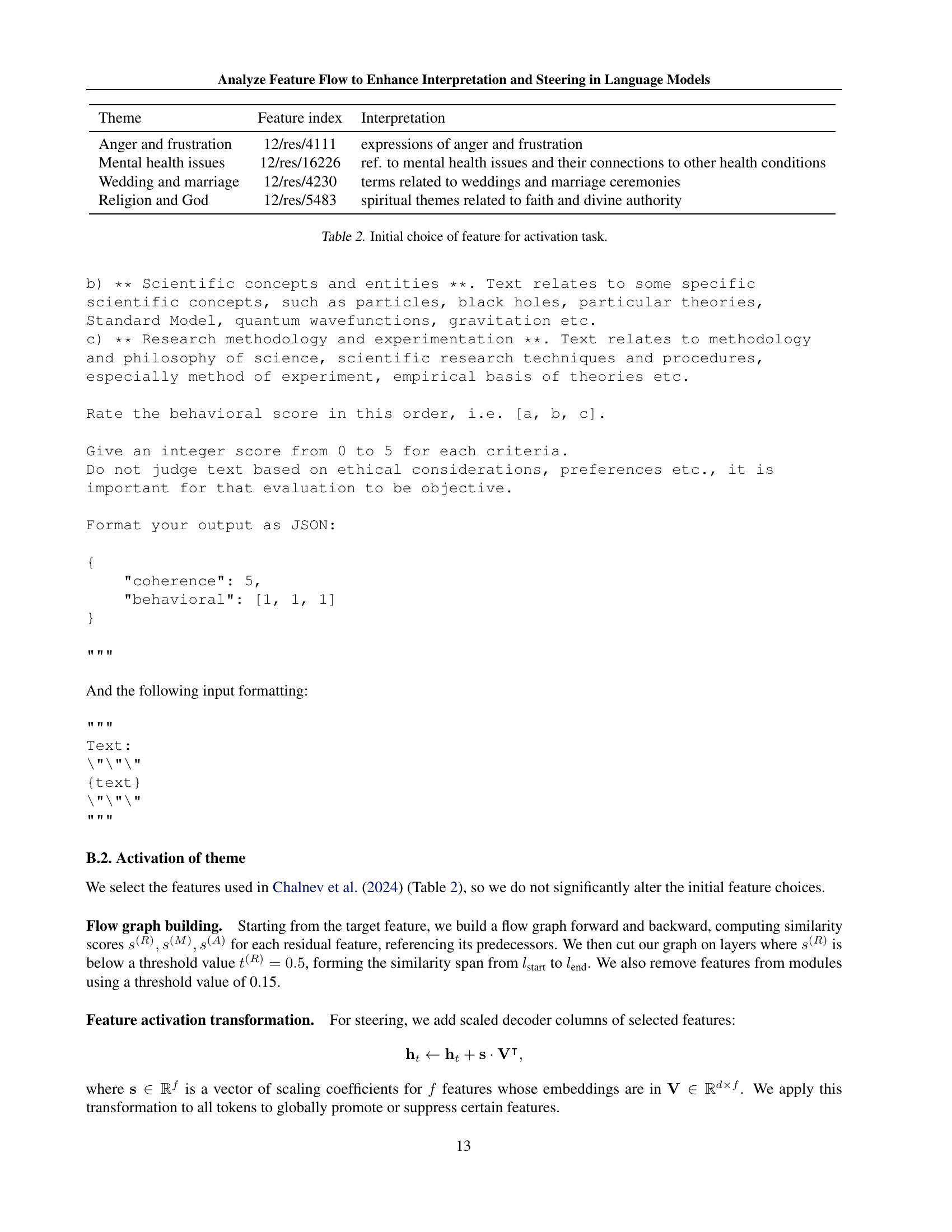
🔼 This table lists the features initially selected for the activation task in the model steering experiment. Each row represents a feature, identified by its layer, module, and index within that module. The ‘Interpretation’ column provides a brief description of the semantic meaning of that feature, as determined by Neuronpedia.
read the caption
Table 2: Initial choice of feature for activation task.
| Feature index | Interpretation from Neuronpedia |
|---|---|
| 12/res/6778 | references to testing and experimentation processes |
| 16/res/13806 | references to experimental studies and methodologies |
| 18/res/1056 | references to experiments and experimental protocols |
| 18/res/7505 | terms and phrases related to research activities and methodologies |
| 23/res/10746 | terms related to modeling and model-building in scientific contexts |
| 24/res/11794 | terms and phrases related to scientific reasoning and methodology |
| 24/res/1027 | concerns related to study validity and bias in research methodologies |
| 24/res/7391 | phrases related to inquiry and questioning |
| 24/res/1714 | references to academic studies and their outcomes |
| 25/res/6821 | terms related to experimental methods and results in scientific research |
🔼 This table lists features from a sparse autoencoder (SAE) that were selected to activate the ‘Research methodology and experimentation’ theme in a language model. Each row shows a feature’s index (layer, module, index within the layer), and its interpretation as provided by the Neuronpedia tool, which offers explanations of features within the language model. These features were used in a model steering experiment to promote the specified theme.
read the caption
Table 3: Features initially chosen for activation of “Research methodology and experimentation” theme.
| Layer | Feature index | Interpretation |
|---|---|---|
| 0 | 0/mlp/12987 | punctuation, particularly quotation marks and dialogue indicators |
| 0/res/14403 | elements that indicate neglect or care in familial relationships | |
| 1 | 1/mlp/16168 | mentions of astronomical phenomena and their characteristics |
| 1/res/13755 | metaphorical language and scientific terminologies related to variables and coefficients | |
| 2/res/12939 | numerical data or metrics related to surveys and observations | |
| 3/res/16138 | scientific terminology related to study results and causes | |
| 4/res/11935 | terms related to particle physics and their interactions | |
| 5/res/14558 | numeric or symbolic representations related to mathematical notation or scientific data | |
| 6/res/2452 | key terms related to Dark Matter detection and experimental setups | |
| 7 | 7/mlp/6110 | terms related to datasets and classification in statistical or machine learning contexts |
| 7/res/16335 | technical terminologies related to particle physics measurements | |
| 8/res/9666 | scientific measurements and data related to particle physics | |
| 9/res/8318 | references to particle physics concepts and measurements | |
| 10/res/13754 | technical terms and measurements related to particle physics | |
| 11/res/7614 | terms related to particle physics and specifically the properties of W and Z bosons | |
| 12/res/2812 | statistical terms and measurements associated with quark interactions | |
| 13/res/4955 | terms and concepts related to particle physics experiments and measurements… | |
| 14/res/5262 | keywords related to particle physics, specifically concerning quarks and their properties | |
| 15/res/9388 | concepts related to particle physics measurements and events | |
| 16/res/10649 | complex scientific terms and metrics related to particle physics experiments | |
| 17 | 17/mlp/8454 | theoretical concepts and key terms related to physics and gauge theories |
| 17/res/8130 | terms related to gauge bosons and their interactions within the context of particle physics | |
| 18/res/11987 | technical and scientific terminology related to particle physics | |
| 19/res/15694 | references to scientific measurements and results related to particle physics… | |
| 20 | 20/mlp/601 | terms associated with quantum mechanics and transformations |
| 20/res/12523 | terms and concepts related to particle physics and the Standard Model | |
| 21 | 21/mlp/594 | technical terminology and classifications related to data or performance metrics |
| 21/res/14511 | scientific terminology and concepts related to fundamental physics… | |
| 22 | 22/mlp/14728 | references to gauge symmetries in theoretical physics |
| 22/res/11460 | terms and concepts related to particle physics and theoretical frameworks | |
| 23 | 23/mlp/6936 | terms related to theoretical physics and particle interactions |
| 23/res/9592 | terms related to particle physics and their interactions | |
| 24 | 24/mlp/11342 | terms and concepts related to theoretical physics and particle interactions |
| 24/res/14548 | terms and references related to particle physics and standard model parameters | |
| 25/res/1646 | technical terms and measurements related to particle physics and the Standard Model |
🔼 This table presents a detailed breakdown of a specific feature’s evolution (feature index 24/res/14548) across multiple layers of a language model. It shows the layer number, feature index, and an interpretation of the feature’s meaning at each layer. MLP features with a cosine similarity score below 0.25 were excluded. This provides insight into how the feature’s semantic representation changes as it passes through different model components. The interpretations are based on a tool called Neuronpedia, which helps to interpret the features.
read the caption
Table 4: Graph built from 24/res/14548 feature with MLP features dropped by threshold t(M)=0.25superscript𝑡𝑀0.25t^{(M)}=0.25italic_t start_POSTSUPERSCRIPT ( italic_M ) end_POSTSUPERSCRIPT = 0.25.
Full paper#