Gold-medalist Performance in Solving Olympiad Geometry with AlphaGeometry2

2502.03544

Yuri Chervonyi et el.

🤗 2025-02-07

TL;DR
#

Solving geometry problems automatically has been a long-standing challenge in AI, with previous approaches often relying on either algebraic bashing or limited symbolic reasoning. These methods struggled to achieve high accuracy and generalizability, particularly on complex Olympiad-level problems. AlphaGeometry, a neuro-symbolic system, showed promise but still had limitations in language coverage, symbolic engine efficiency, and overall solve rate.

This paper introduces AlphaGeometry2, a substantial upgrade that addresses these limitations. AlphaGeometry2 achieves a significant performance boost through several key improvements: an expanded domain-specific language to tackle harder problems, a more efficient and robust symbolic engine (DDAR), a novel knowledge-sharing search algorithm (SKEST), and an enhanced language model built upon the Gemini architecture. These advancements enable AlphaGeometry2 to solve 84% of IMO geometry problems from 2000-2024 and surpasses the performance of human gold medalists. The paper also demonstrates progress towards a fully automated system using natural language input.

Key Takeaways
#

Why does it matter?
#

This paper is important because it presents a significant advancement in automated geometry problem-solving, a challenging area with implications for AI, mathematics education, and theorem proving. AlphaGeometry2’s gold-medal performance demonstrates the potential of neuro-symbolic AI systems and opens exciting new research avenues in combining language models, symbolic reasoning, and search algorithms for complex problem-solving. The techniques developed could inspire progress in other fields requiring similar combinations of reasoning abilities.

Visual Insights
#

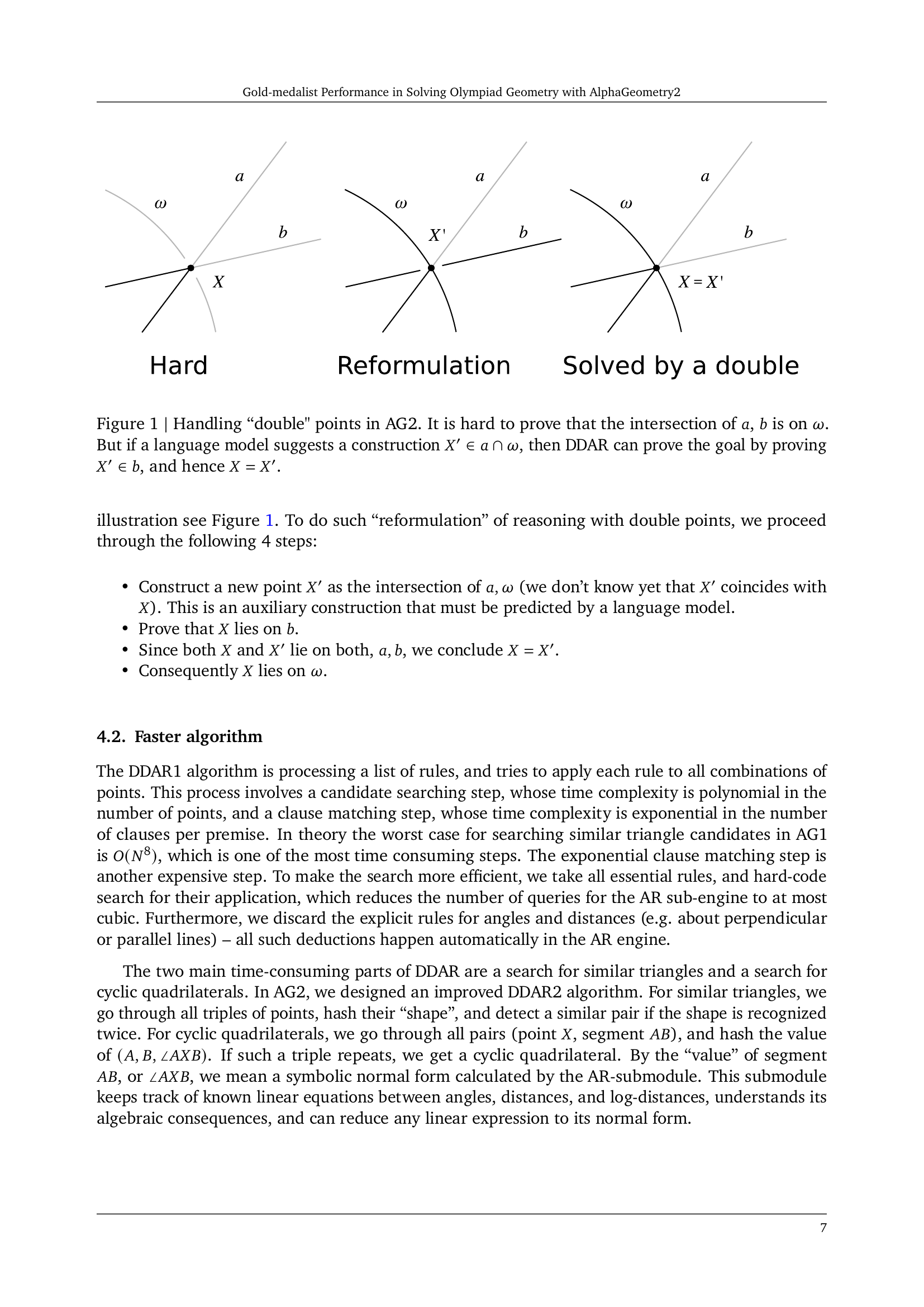
🔼 The figure illustrates how AlphaGeometry2 handles situations where two points share the same coordinates. A common geometry problem involves proving that a point X is on a circle ωω ω. However, X is defined as the intersection of two lines. Directly proving X lies on ωω ω is difficult for a symbolic engine. Instead, a language model suggests constructing an auxiliary point X′X′ that’s also at the intersection of line a and circle ωω ω. Then, AlphaGeometry2 proves that X′X′ is on line b. Because X and X′X′ share coordinates, and both are on line b and a, this indirectly proves that the original point X lies on ωω ω.
read the caption
Figure 1: Handling “double' points in AG2. It is hard to prove that the intersection of a𝑎aitalic_a, b𝑏bitalic_b is on ω𝜔\omegaitalic_ω. But if a language model suggests a construction X′∈a∩ωsuperscript𝑋′𝑎𝜔X^{\prime}\in a\cap\omegaitalic_X start_POSTSUPERSCRIPT ′ end_POSTSUPERSCRIPT ∈ italic_a ∩ italic_ω, then DDAR can prove the goal by proving X′∈bsuperscript𝑋′𝑏X^{\prime}\in bitalic_X start_POSTSUPERSCRIPT ′ end_POSTSUPERSCRIPT ∈ italic_b, and hence X=X′𝑋superscript𝑋′X=X^{\prime}italic_X = italic_X start_POSTSUPERSCRIPT ′ end_POSTSUPERSCRIPT.

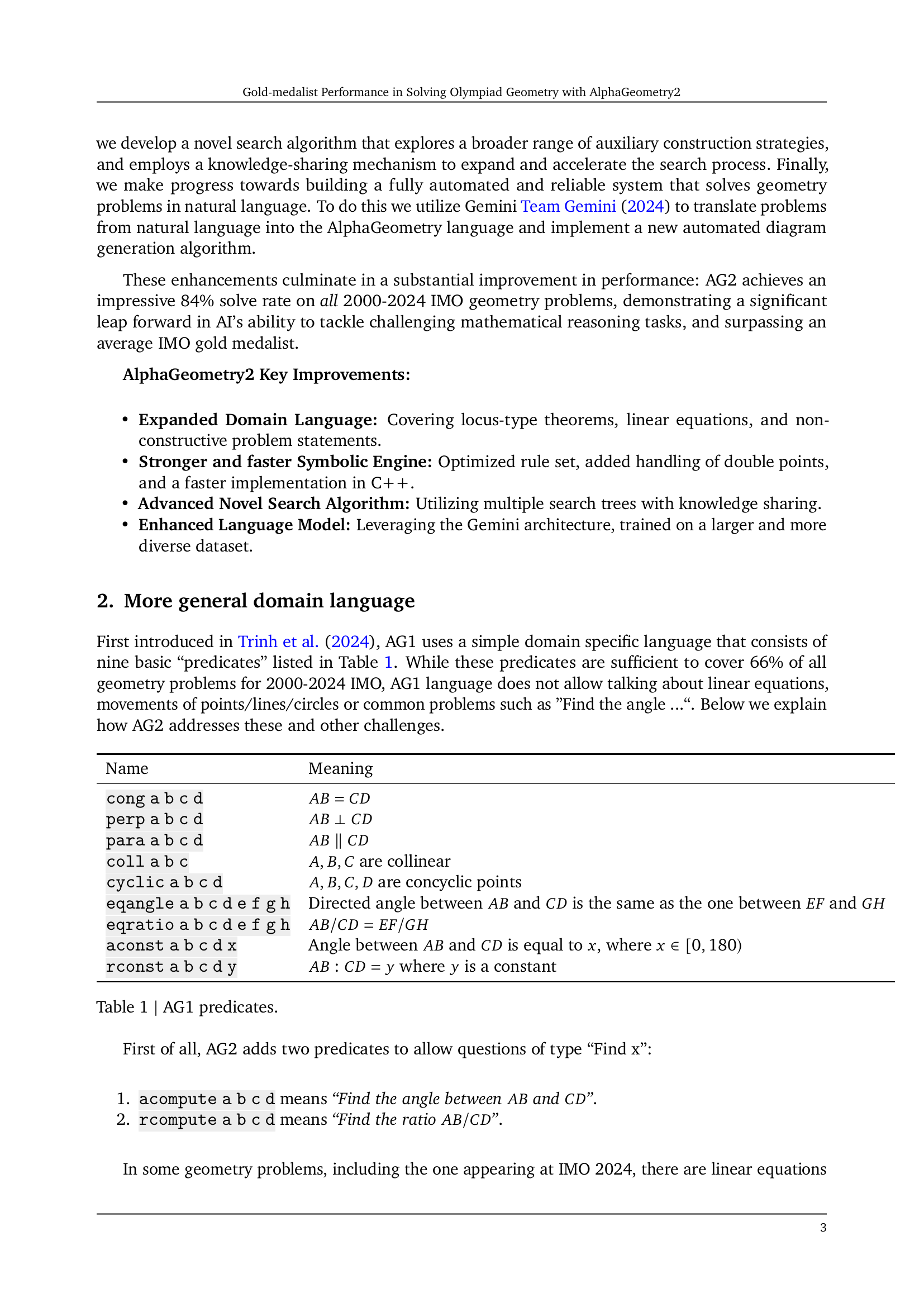
Name	Meaning
cong a b c d	$AB=CD$
perp a b c d	$AB\perp CD$
para a b c d	$AB\parallel CD$
coll a b c	$A,B,C$ are collinear
cyclic a b c d	$A,B,C,D$ are concyclic points
eqangle a b c d e f g h	Directed angle between $AB$ and $CD$ is the same as the one between $EF$ and $GH$
eqratio a b c d e f g h	$AB/CD=EF/GH$
aconst a b c d x	Angle between $AB$ and $CD$ is equal to $x$ , where $x\in[0,180)$
rconst a b c d y	$AB:CD=y$ where $y$ is a constant

🔼 This table lists the nine predicates used in the AlphaGeometry1 (AG1) domain-specific language for representing geometric relationships. Each predicate encodes a specific geometric concept, such as equality of lengths, parallelism, collinearity, or concyclic points. These predicates form the basic building blocks for expressing geometry problems within the AG1 system.
read the caption
Table 1: AG1 predicates.

In-depth insights
#

Neuro-Symbolic AI
#

Neuro-symbolic AI integrates the strengths of neural networks and symbolic reasoning to overcome limitations of each individual approach. Neural networks excel at learning complex patterns from data, but lack explainability and struggle with reasoning and symbolic manipulation. Symbolic AI excels at explicit knowledge representation and logical inference, but requires extensive manual encoding of knowledge and doesn’t readily adapt to new, unseen data. Neuro-symbolic AI aims to bridge this gap by combining the pattern recognition power of neural networks with the reasoning capabilities of symbolic systems. This often involves using neural networks to learn representations that can then be used by symbolic reasoners, or using symbolic constraints to guide the learning of neural networks. The result is a system that can learn from data, reason logically, and provide explanations for its decisions. This approach holds significant promise for applications demanding both high accuracy and transparency, such as medical diagnosis, robotics, and scientific discovery.

Gemini Language Model
#

The research paper highlights the crucial role of the Gemini language model in significantly enhancing the capabilities of AlphaGeometry2. Gemini’s superior architecture provides better language modeling compared to its predecessor, enabling more accurate and comprehensive understanding of geometry problems. This improved understanding directly translates to enhanced problem formalization and diagram generation, allowing the system to more effectively tackle complex geometrical concepts. The model’s training on a larger and more diverse dataset further contributes to its performance gains, which are demonstrated by AlphaGeometry2’s ability to surpass the average gold medalist in solving Olympiad geometry problems. The integration of Gemini is therefore a key innovation that showcases the potential of large language models to solve complex mathematical tasks and improves the overall solving rate.

Automated Diagram Generation
#

The section on “Automated Diagram Generation” in the research paper reveals a crucial advancement in automating geometry problem-solving. The authors address the challenge of generating diagrams from non-constructive problem statements, where points aren’t easily defined by simple intersections. Their proposed solution uses a two-step optimization method: first, a gradient descent to establish initial point coordinates, followed by a Gauss-Newton-Levenberg refinement for accuracy. This approach is benchmarked on 44 IMO problems, achieving a high success rate. The automation of diagram generation is vital; it eliminates a significant manual step, enabling the system to handle a wider variety of geometry problems, especially non-constructive ones. This automated process directly impacts the overall efficiency and scalability of the system, significantly contributing to the improved success rate in solving IMO geometry problems reported in the study. The method shows that even with non-constructive problem statements, diagrams are reliably generated through numerical approaches, a significant contribution to advancing automated geometry theorem proving.

DDAR Enhancements
#

The research paper section on ‘DDAR Enhancements’ would likely detail improvements to the Deductive Database Arithmetic Reasoning (DDAR) system, a core component for solving geometry problems. Key improvements could include enhanced handling of double points, addressing situations where distinct points share the same coordinates. This might involve algorithmic changes to the deduction closure process, allowing for more robust and complete solutions in complex scenarios. The section would likely also describe a faster algorithm for DDAR, possibly achieved through optimized rule sets or streamlined search strategies. The goal would be to reduce computation time and enable the exploration of a broader search space. Finally, faster implementation, perhaps using a more efficient programming language like C++, would significantly improve the system’s speed, leading to quicker solutions and increased capacity to handle larger and more complex geometry problems. Overall, these enhancements aim to increase the accuracy, efficiency and robustness of AlphaGeometry2’s symbolic engine, ultimately boosting its performance in solving geometry problems.

Future Research
#

Future research directions stemming from this gold-medal performance in solving Olympiad geometry problems using AlphaGeometry2 could explore several key areas. Improving the language model’s ability to handle inequalities and problems with variable numbers of points is crucial for broader applicability. Developing more sophisticated techniques for diagram generation, especially for non-constructive problems, is essential. The research could investigate more advanced symbolic reasoning techniques capable of handling complex geometric relationships and more efficiently managing the deductive process. Exploring the integration of reinforcement learning to improve problem decomposition and the learning of advanced geometric problem-solving strategies warrants further investigation. Finally, a particularly interesting avenue for future work would be to thoroughly investigate the potential of multi-modal approaches that integrate visual information from diagrams to enhance accuracy and efficiency. This would leverage the strength of Gemini’s multi-modal capabilities for a comprehensive approach. The insights gained from this research could benefit not only mathematics but also broader AI research in complex reasoning.

More visual insights
#

More on figures

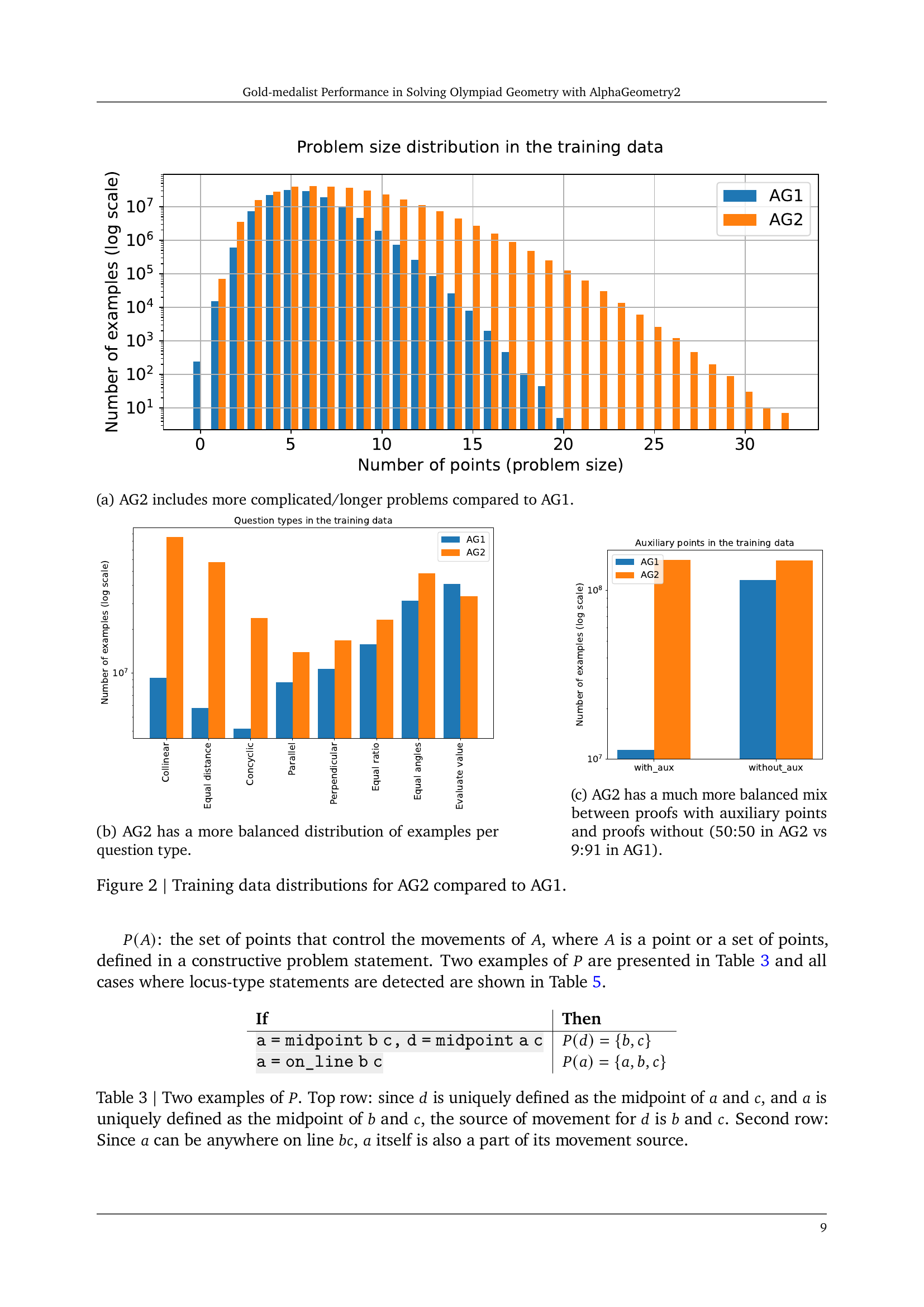
🔼 This figure shows a comparison of problem size distributions in the training data for AlphaGeometry1 (AG1) and AlphaGeometry2 (AG2). The x-axis represents the number of points in a geometry problem, indicating its complexity. The y-axis shows the number of problems of each size in the training data. The bars show that AG2’s training data contains a significantly larger number of problems with a higher number of points, indicating that AG2 was trained on more complex geometry problems than AG1. This difference is visually apparent, showing AG2 trained on more complex problems and thus providing a rationale for its improved performance.
read the caption
(a) AG2 includes more complicated/longer problems compared to AG1.

🔼 This figure shows a bar chart comparing the distribution of question types in the training data of AlphaGeometry1 (AG1) and AlphaGeometry2 (AG2). AlphaGeometry2 demonstrates a more even distribution across various geometry problem types, unlike AG1 which shows a skewed distribution. This balance in AG2’s training data ensures the model is exposed to a more diverse range of geometry problem characteristics, thus leading to improved performance and generalization.
read the caption
(b) AG2 has a more balanced distribution of examples per question type.

🔼 The figure shows a comparison of the distribution of auxiliary points in the training data between AlphaGeometry1 (AG1) and AlphaGeometry2 (AG2). AG1 has a highly skewed distribution, with only 9% of the problems using auxiliary points. In contrast, AG2 has a significantly more balanced distribution, with approximately 50% of the problems utilizing auxiliary points.
read the caption
(c) AG2 has a much more balanced mix between proofs with auxiliary points and proofs without (50:50 in AG2 vs 9:91 in AG1).

🔼 This figure compares the training data distributions of AlphaGeometry 1 (AG1) and AlphaGeometry 2 (AG2). Panel (a) shows a bar chart illustrating the distribution of problem sizes (number of points) in the training data for both AG1 and AG2. AG2 includes more problems with a higher number of points, indicating a larger and more complex dataset. Panel (b) displays a bar chart comparing the distribution of question types in AG1 and AG2 training data. AG2 shows a more balanced distribution across different question types, unlike AG1 which was skewed. Panel (c) shows a bar chart comparing the distribution of problems with and without auxiliary points in the AG1 and AG2 training sets. AG2 exhibits a much more balanced distribution (approximately 50/50) compared to AG1 (9/91). Overall, the figure demonstrates that AG2’s training data is both larger and more diverse than that of AG1, improving the model’s ability to handle a wider range of problem complexities and types.
read the caption
Figure 2: Training data distributions for AG2 compared to AG1.

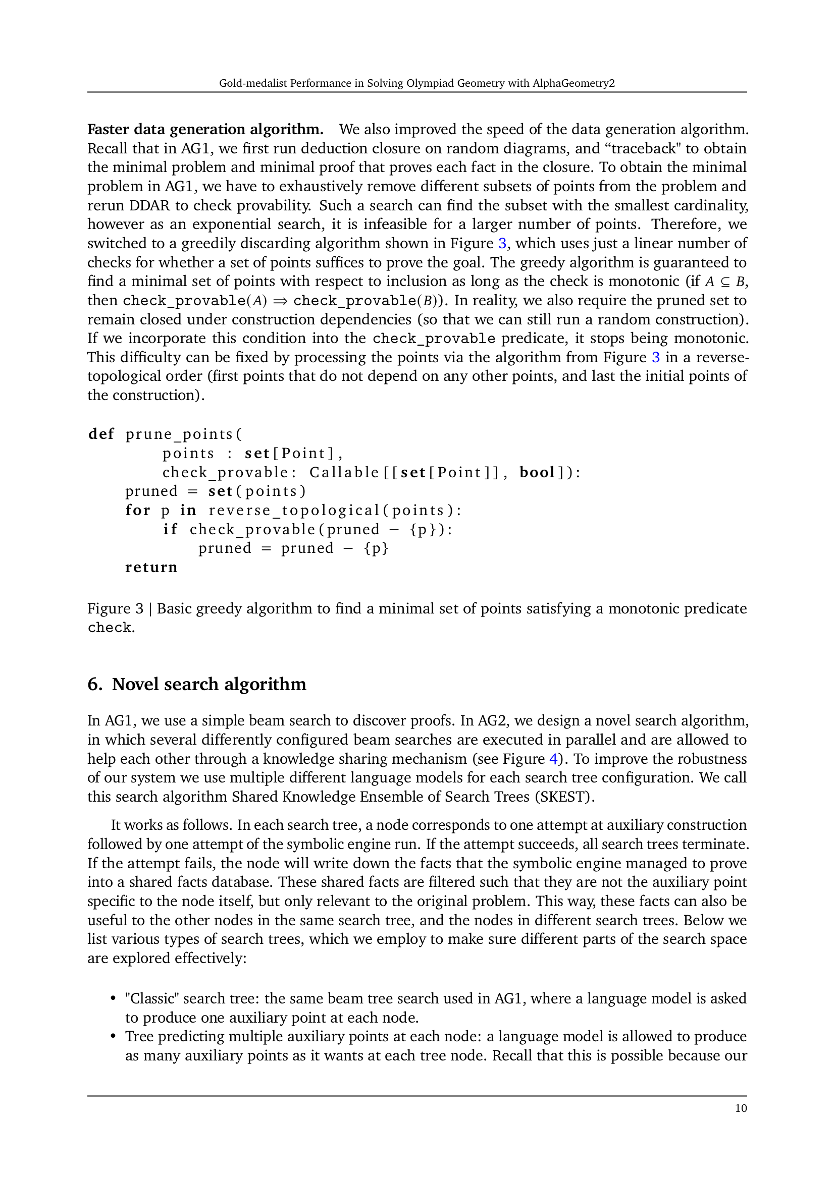
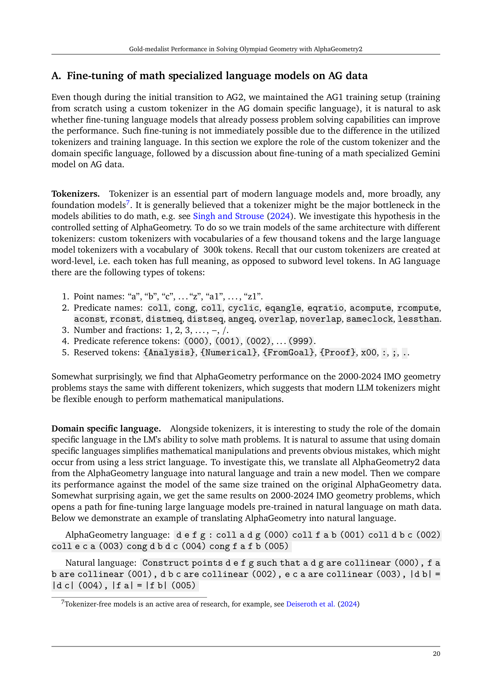
🔼 This figure presents a Python function named prune_points. The function takes a set of points and a function check_provable as input. check_provable is a function that determines if a given subset of points satisfies a specific condition (a ‘monotonic predicate’). The algorithm iterates through the points in reverse topological order (meaning it starts with points that don’t depend on others for their definition). In each iteration, it checks if removing the current point still allows check_provable to return true. If it does, the point is removed from the set of points (pruned). The function returns the minimal set of points that still satisfy the condition. This greedy approach efficiently finds a minimal set of points, ensuring that the condition remains true without unnecessary points.
read the caption
Figure 3: Basic greedy algorithm to find a minimal set of points satisfying a monotonic predicate check.

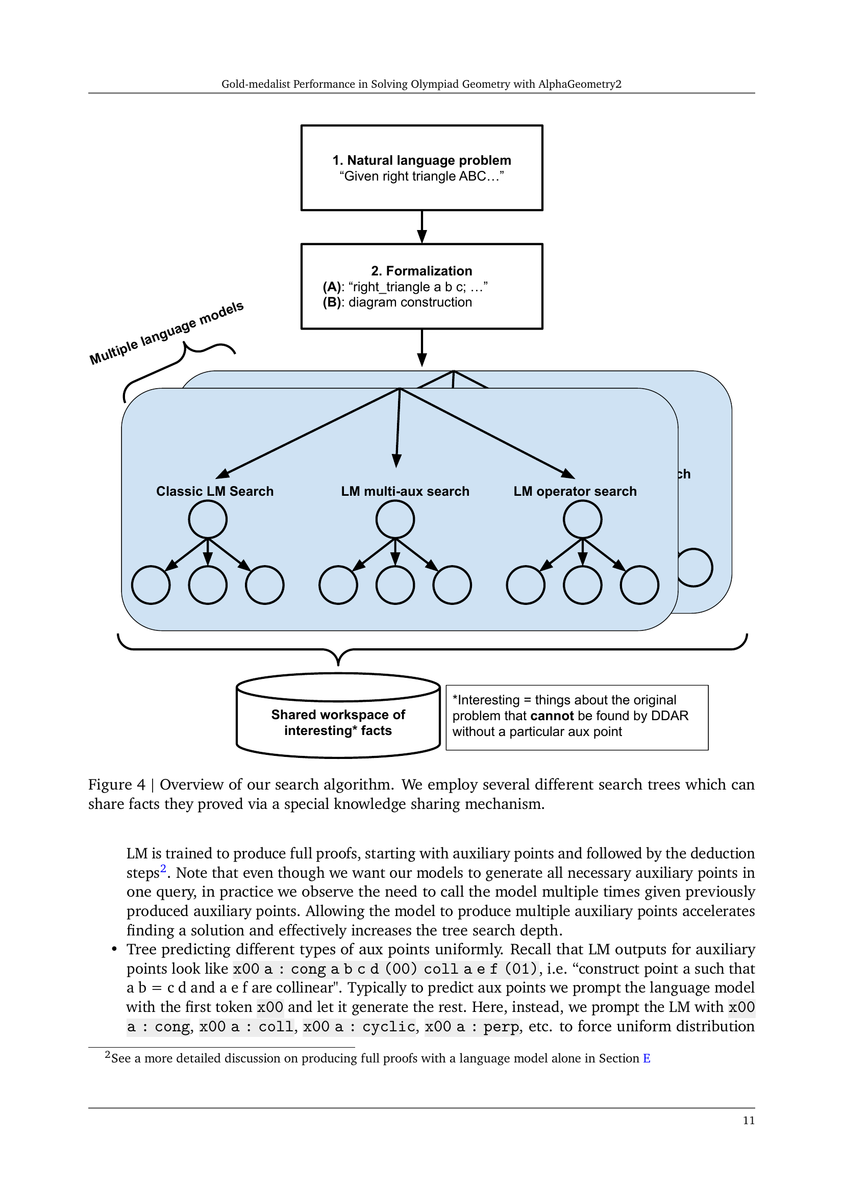
🔼 The figure illustrates the AlphaGeometry2 search algorithm, called Shared Knowledge Ensemble of Search Trees (SKEST). Instead of using a single search tree, the algorithm employs multiple search trees, each with a different configuration (e.g., classic beam search, multi-auxiliary point search, operator search). These trees operate in parallel and share proven facts through a central knowledge base. This shared knowledge accelerates the search process and enhances the robustness of the system by allowing different search strategies to complement each other.
read the caption
Figure 4: Overview of our search algorithm. We employ several different search trees which can share facts they proved via a special knowledge sharing mechanism.

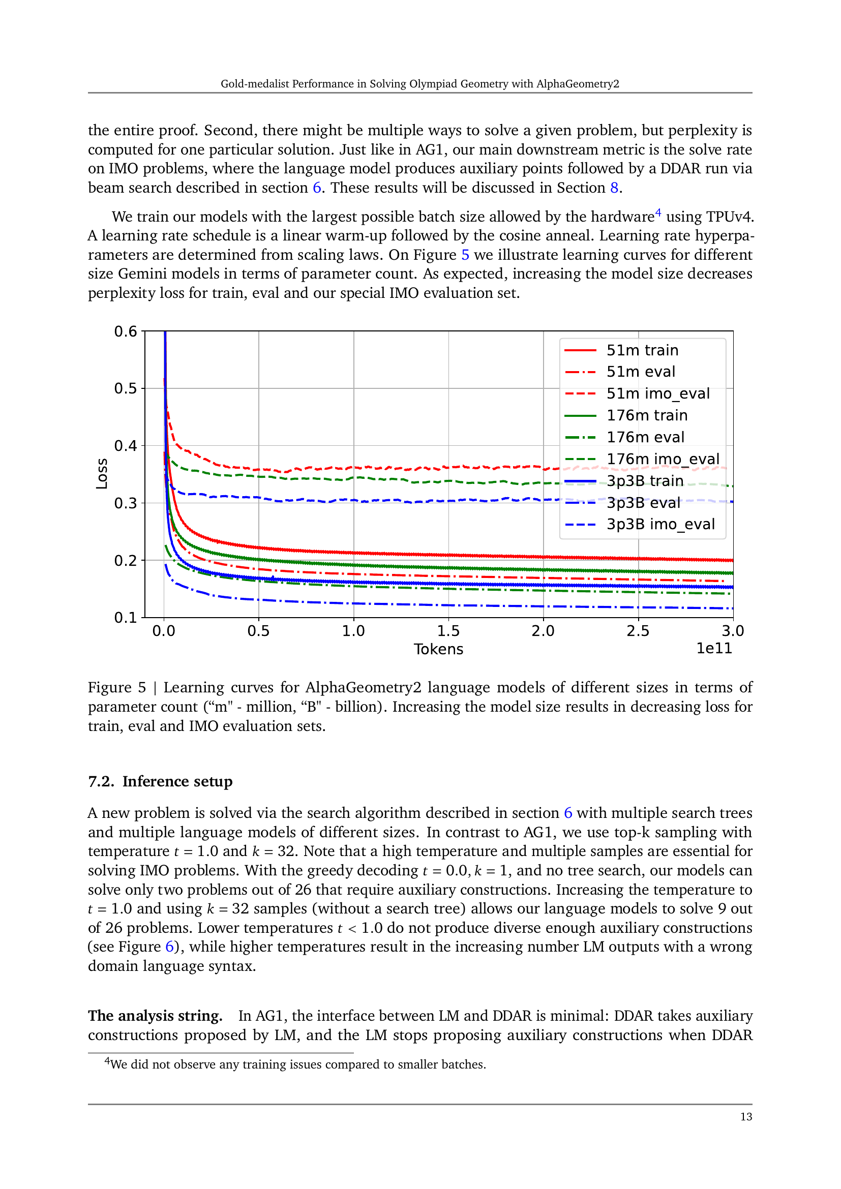
🔼 This figure shows the learning curves for three AlphaGeometry2 language models with different numbers of parameters (51 million, 176 million, and 3.3 billion). The x-axis represents the number of tokens processed during training, and the y-axis represents the loss. Three curves are shown for each model: one for the training data, one for a held-out evaluation dataset, and one specifically for the International Mathematical Olympiad (IMO) evaluation dataset. The results indicate that as the model size increases, the loss consistently decreases across all three datasets (train, eval, and IMO). This demonstrates improved model performance with a larger number of parameters.
read the caption
Figure 5: Learning curves for AlphaGeometry2 language models of different sizes in terms of parameter count (“m' - million, “B' - billion). Increasing the model size results in decreasing loss for train, eval and IMO evaluation sets.

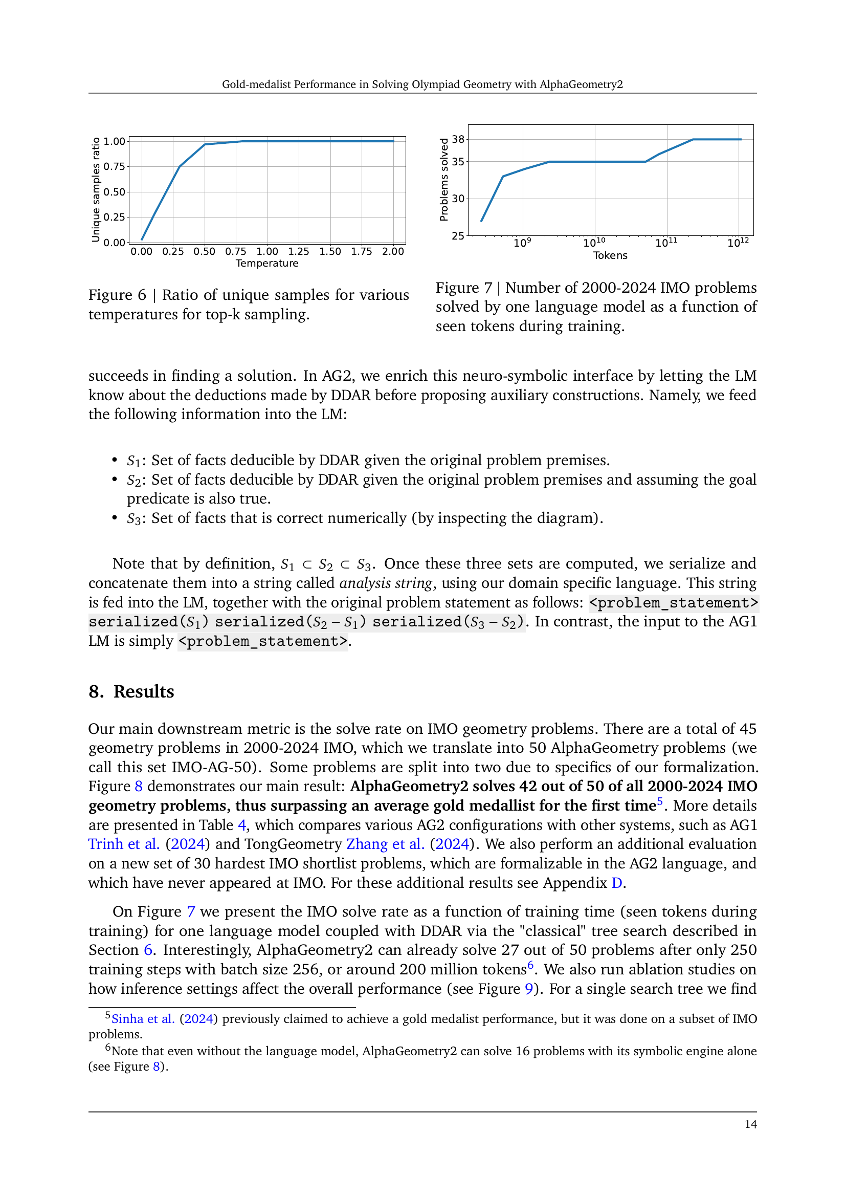
🔼 This figure shows the impact of temperature on the diversity of samples generated using top-k sampling. The x-axis represents the temperature values, and the y-axis shows the ratio of unique samples obtained for each temperature. As temperature increases, the ratio of unique samples also increases, indicating that higher temperatures lead to more diverse samples. This demonstrates the effect of temperature as a hyperparameter in controlling the randomness of the sampling process.
read the caption
Figure 6: Ratio of unique samples for various temperatures for top-k sampling.

🔼 This figure shows the relationship between the number of 2000-2024 International Mathematical Olympiad (IMO) geometry problems solved by a single language model and the amount of data (measured in tokens) it has been trained on. It illustrates how the model’s problem-solving ability improves as it is exposed to more training data.
read the caption
Figure 7: Number of 2000-2024 IMO problems solved by one language model as a function of seen tokens during training.

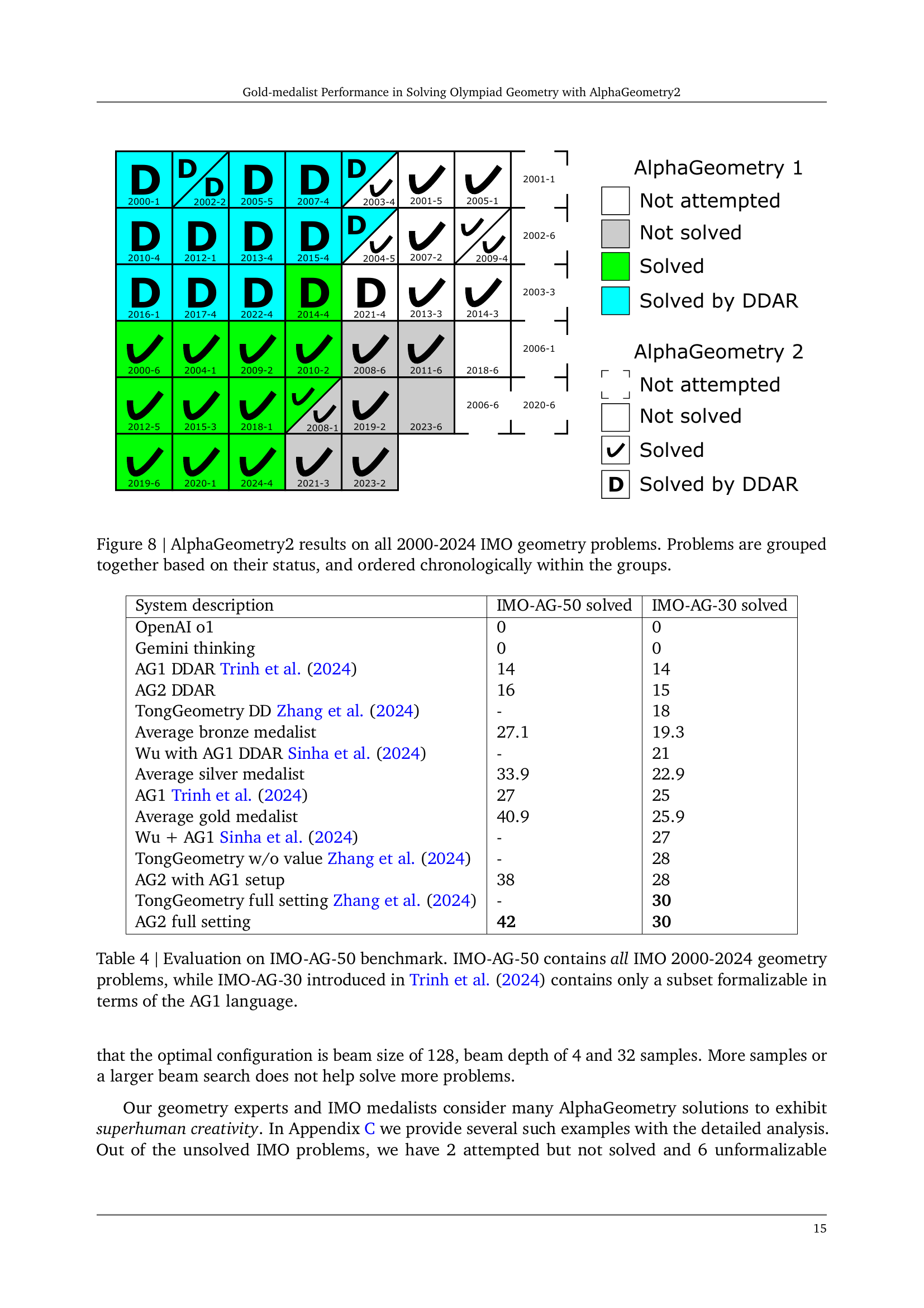
🔼 This figure presents a visual representation of AlphaGeometry2’s performance on International Mathematical Olympiad (IMO) geometry problems from 2000 to 2024. Each problem is categorized into one of three groups: ‘Not Attempted’, ‘Not Solved’, and ‘Solved’. Within each group, problems are chronologically ordered, providing a clear visualization of the system’s progress over time. The use of a visual matrix aids in understanding AlphaGeometry2’s success rate on various problems and highlights which problems were successfully solved using only a deductive database arithmetic reasoning (DDAR) engine, without the need for a language model.
read the caption
Figure 8: AlphaGeometry2 results on all 2000-2024 IMO geometry problems. Problems are grouped together based on their status, and ordered chronologically within the groups.

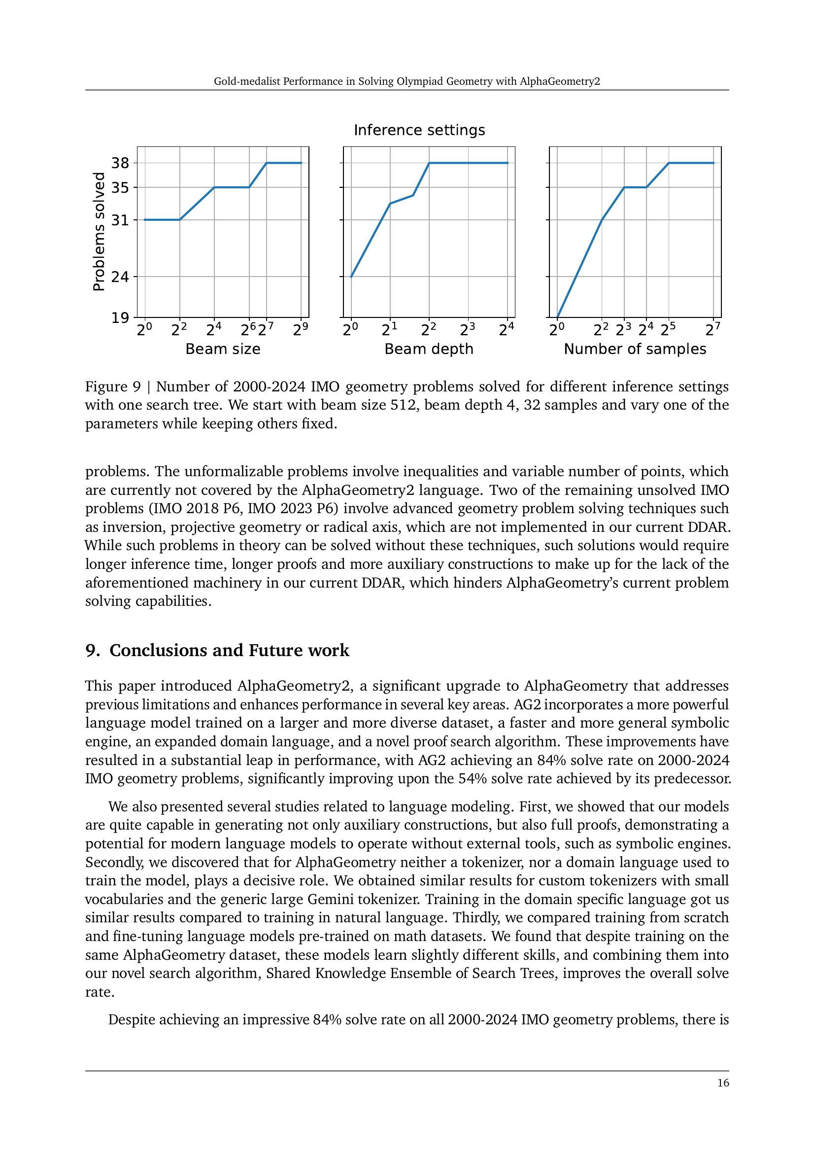
🔼 This figure displays the impact of different inference settings on the number of solved 2000-2024 IMO geometry problems. The experiment uses a single search tree and systematically varies one parameter (beam size, beam depth, or number of samples) while holding the others constant at their initial values (beam size=512, beam depth=4, number of samples=32). The results are presented as a graph showing the count of problems solved for each parameter setting variation, allowing for a clear visual comparison of the effectiveness of each setting.
read the caption
Figure 9: Number of 2000-2024 IMO geometry problems solved for different inference settings with one search tree. We start with beam size 512, beam depth 4, 32 samples and vary one of the parameters while keeping others fixed.

🔼 This figure displays the learning curves for two 3-billion parameter language models. One model was trained from scratch, while the other was initially pre-trained on mathematical datasets before undergoing fine-tuning on AlphaGeometry (AG) data. The plot shows the loss values over the training process, measured in terms of the number of tokens processed. Notably, the model that started with pre-training on math data exhibits a lower initial loss. However, both models eventually converge to a similar loss level after training with 200 billion tokens.
read the caption
Figure 10: Learning curves for two 3B models: one is trained from scratch and another one pre-trained on math data and then fine-tuned on the AG data. The model pre-trained on math has initially lower loss but both converge to the same point after training for 200B tokens.

🔼 The figure displays the diagram for problem IMO 2024 P4, enhanced with AlphaGeometry’s auxiliary construction point E. This problem involves a triangle ABC with incenter I, where AB < AC < BC. Point X lies on line BC (excluding C), such that the line through X parallel to AC is tangent to the incircle. Similarly, point Y lies on BC (excluding B) such that the line through Y parallel to AB is tangent to the incircle. Line AI intersects the circumcircle of triangle ABC at point P. K and L are midpoints of AC and AB, respectively. The problem’s objective is to prove that ∠KIL + ∠YPX = 180°. Point E, added by AlphaGeometry, is crucial to solving this complex geometry problem. The diagram illustrates the geometric relationships between the various points and lines involved, highlighting the auxiliary construction.
read the caption
Figure 11: IMO 2024 P4 diagram with AlphaGeometry auxiliary construction, point E𝐸Eitalic_E.

🔼 Figure 12 shows the diagram for IMO 2013 Problem 3, enhanced with the auxiliary point D added by AlphaGeometry2. The key insight provided by AlphaGeometry2 is identifying that points B, A₁ (A sub 1), D, and Iₐ (I sub a) are concyclic (lie on the same circle). This is a crucial step in solving the problem. The figure visually demonstrates this concyclicity and other geometric elements used in the proof.
read the caption
Figure 12: IMO 2013 P3 diagram with AlphaGeometry auxiliary construction, point D𝐷Ditalic_D. It allows proving B⁢A1⁢D⁢Ia𝐵subscript𝐴1𝐷subscript𝐼𝑎BA_{1}DI_{a}italic_B italic_A start_POSTSUBSCRIPT 1 end_POSTSUBSCRIPT italic_D italic_I start_POSTSUBSCRIPT italic_a end_POSTSUBSCRIPT is cyclic, which is the key to solve this problem.

🔼 This figure shows the diagram for problem 3 from the 2014 International Mathematical Olympiad (IMO) as interpreted by AlphaGeometry2. The diagram includes the original problem’s points and lines, as well as additional points and lines constructed by AlphaGeometry2’s algorithm to aid in solving the problem. These auxiliary constructions, added by the AI system, illustrate the steps of its reasoning process and are crucial to the solution path it found.
read the caption
Figure 13: IMO 2014 P3 diagram with AlphaGeometry auxiliary constructions.

🔼 This figure shows the solution to problem G7 from the 2009 International Mathematical Olympiad shortlist, as solved by AlphaGeometry2. The diagram displays triangle ABC with its incenter I, and the incenters X, Y, and Z of triangles BIC, CIA, and AIB respectively. AlphaGeometry2’s auxiliary constructions (shown in red) are used to create several key cyclic quadrilaterals (colored polygons) and similar triangle pairs (colored triangle pairs). These geometric relationships are crucial for proving that if triangle XYZ is equilateral, then triangle ABC must also be equilateral. The colored elements highlight the key geometric properties and relationships exploited by AlphaGeometry2 in its solution.
read the caption
Figure 14: IMOSL 2009 G7 diagram with AlphaGeometry auxiliary constructions (colored red), key cyclic properties (colored polygons) and key similar triangle pairs (colored triangle pairs).

More on tables

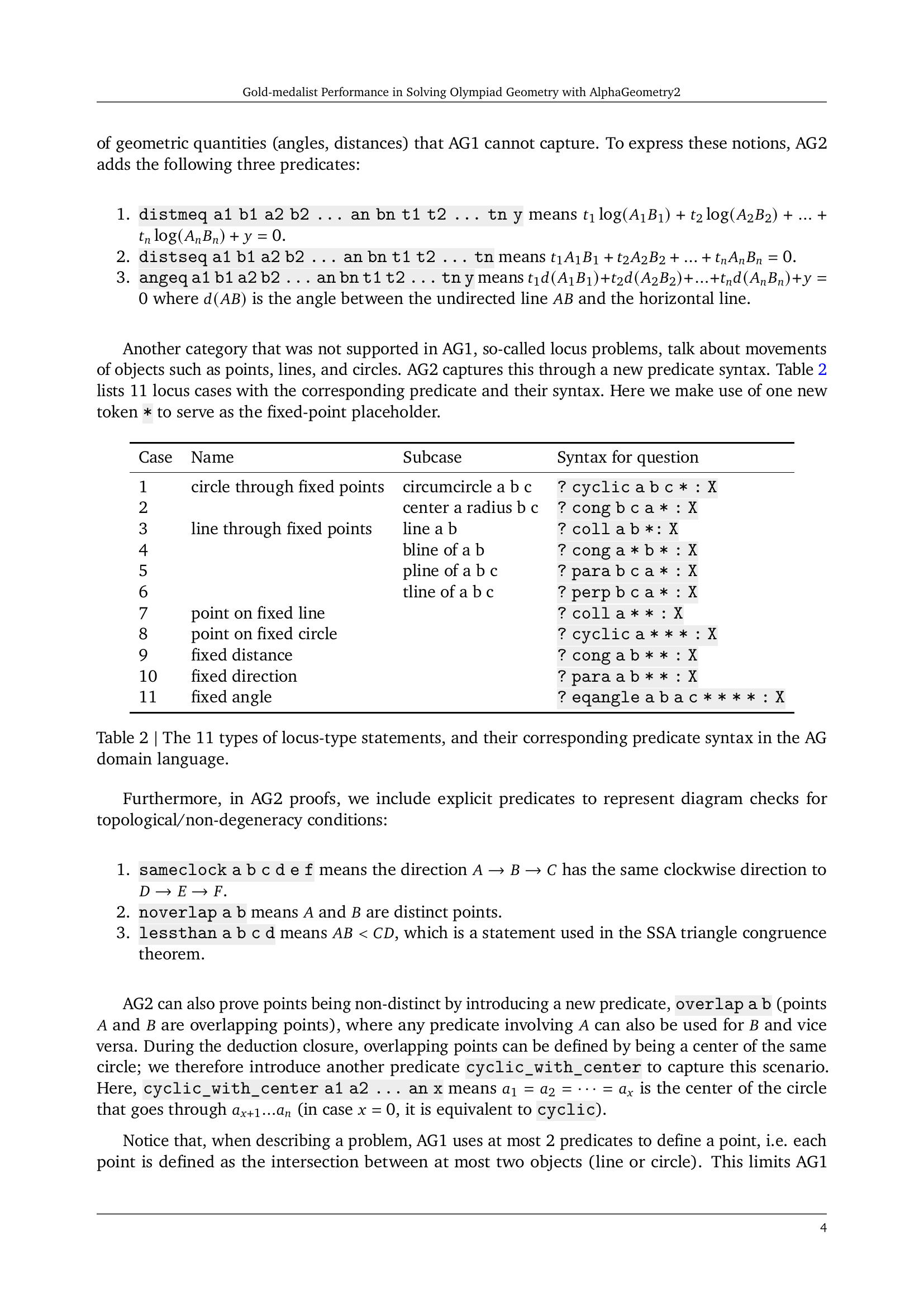
Case	Name	Subcase	Syntax for question
1	circle through fixed points	circumcircle a b c	? cyclic a b c * : X
2		center a radius b c	? cong b c a * : X
3	line through fixed points	line a b	? coll a b *: X
4		bline of a b	? cong a * b * : X
5		pline of a b c	? para b c a * : X
6		tline of a b c	? perp b c a * : X
7	point on fixed line		? coll a * * : X
8	point on fixed circle		? cyclic a * * * : X
9	fixed distance		? cong a b * * : X
10	fixed direction		? para a b * * : X
11	fixed angle		? eqangle a b a c * * * * : X

🔼 This table lists eleven different types of locus statements that can appear in geometry problems, along with their corresponding predicates in the AlphaGeometry2 (AG2) domain-specific language. Each row shows a type of locus statement, the subcase describing it, and its representation as a predicate in the AG2 language. The syntax for how questions are formed is shown using an example including the ‘?’ symbol, which is followed by a series of terms that indicate specific points and relationships, and lastly the variable ‘X’ to be solved for. This helps illustrate how AG2 handles the complexities of locus problems.
read the caption
Table 2: The 11 types of locus-type statements, and their corresponding predicate syntax in the AG domain language.

If	Then
a = midpoint b c, d = midpoint a c	$P(d)=\{b,c\}$
a = on_line b c	$P(a)=\{a,b,c\}$

🔼 This table illustrates how the function P(A), representing the set of points controlling the movement of point A, is determined. The top row shows a case where point d is defined as the midpoint of a and c, and point a is the midpoint of b and c. Because of these dependencies, the movement of d is controlled by b and c. The bottom row shows a case where point a lies on a line defined by points b and c, meaning point a itself directly determines its own movement, thus a is included in its own controlling set.
read the caption
Table 3: Two examples of P𝑃Pitalic_P. Top row: since d𝑑ditalic_d is uniquely defined as the midpoint of a𝑎aitalic_a and c𝑐citalic_c, and a𝑎aitalic_a is uniquely defined as the midpoint of b𝑏bitalic_b and c𝑐citalic_c, the source of movement for d𝑑ditalic_d is b𝑏bitalic_b and c𝑐citalic_c. Second row: Since a𝑎aitalic_a can be anywhere on line b⁢c𝑏𝑐bcitalic_b italic_c, a𝑎aitalic_a itself is also a part of its movement source.

System description	IMO-AG-50 solved	IMO-AG-30 solved
OpenAI o1	0	0
Gemini thinking	0	0
AG1 DDAR Trinh et al. (2024)	14	14
AG2 DDAR	16	15
TongGeometry DD Zhang et al. (2024)	-	18
Average bronze medalist	27.1	19.3
Wu with AG1 DDAR Sinha et al. (2024)	-	21
Average silver medalist	33.9	22.9
AG1 Trinh et al. (2024)	27	25
Average gold medalist	40.9	25.9
Wu + AG1 Sinha et al. (2024)	-	27
TongGeometry w/o value Zhang et al. (2024)	-	28
AG2 with AG1 setup	38	28
TongGeometry full setting Zhang et al. (2024)	-	30
AG2 full setting	42	30

🔼 Table 4 presents a comparison of the performance of various geometry problem-solving systems on two benchmarks: IMO-AG-50 and IMO-AG-30. IMO-AG-50 includes all International Mathematical Olympiad (IMO) geometry problems from 2000 to 2024, while IMO-AG-30 is a subset of these problems that are expressible using the AlphaGeometry 1 language. The table compares different systems, including AlphaGeometry 1 and 2, along with other state-of-the-art methods, showing their respective solution counts for each benchmark. This allows for assessing the improvement achieved by AlphaGeometry 2 over previous models and other systems.
read the caption
Table 4: Evaluation on IMO-AG-50 benchmark. IMO-AG-50 contains all IMO 2000-2024 geometry problems, while IMO-AG-30 introduced in Trinh et al. (2024) contains only a subset formalizable in terms of the AG1 language.

Given a random diagram, if DDAR proves:	Then let X =	Then if X is nonempty, we create a synthetic proof that says: "when X moves, …	Auxiliary constructions will be the following points and everything else they depend on	Case
cong a b c d	$P(b,c,d)-P(a)$	circle center $b$ , radius $cd$ goes through a fixed point	$a$	2
	$P(a)-P(b,c,d)$	$a$ moves on a fixed circle	$b,c,d$	8
	$P(a,b)-P(c,d)$	the distance between $a$ and $b$ is fixed	$c,d$	9
cong a b a c	$P(a)-P(b,c)$	$a$ moves on a fixed line	$b,c$	7
	$P(b,c)-P(a)\geq M$	$b$ & $c$ are equidistant to a fixed point, when M move	$a$	4
cyclic a b c d	$P(b,c,d)-P(a)$	the circumcircle of $b$ $c$ $d$ moves through a fixed point	$a$	1
	$P(d)-P(a,b,c)$	$d$ moves on a fixed circle	$a,b,c$	8
coll a b c	$P(b,c)-P(a)$	line $b$ $c$ goes through a fixed point	$a$	3
	$P(c)-P(a,b)$	$c$ moves on a fixed line	$a,b$	7
eqangle b a b c e d e f	$P(a,b,c)-P(d,e,f)$	the angle $a$ $b$ $c$ has a fixed value	$d,e,f$	11
	$P(b)-P(a,c,d,e,f)$	the point $b$ moves on a fixed circle	$a,c,d,e,f$	8
para a b c d	$P(b,c,d)-P(a)$	The line through $b$ and $\parallel cd$ moves through a fixed point	$a$	5
	$P(c,d)-P(a,b)$	The line $cd$ is always parallel to a fixed line	$a,b$	10
	$P(a)-P(b,c,d)$	$a$ moves on a fixed line	$b,c,d$	7
perp a b c d	$P(b,c,d)-P(a)$	the line through $b$ and $\perp cd$ moves through fixed point	$a$	6
	$P(c,d)-P(a,b)$	the line $cd$ is always $\perp$ to a fixed line	$a,b$	10
	$P(a)-P(b,c,d)$	$a$ moves on a fixed line	$b,c,d$	7

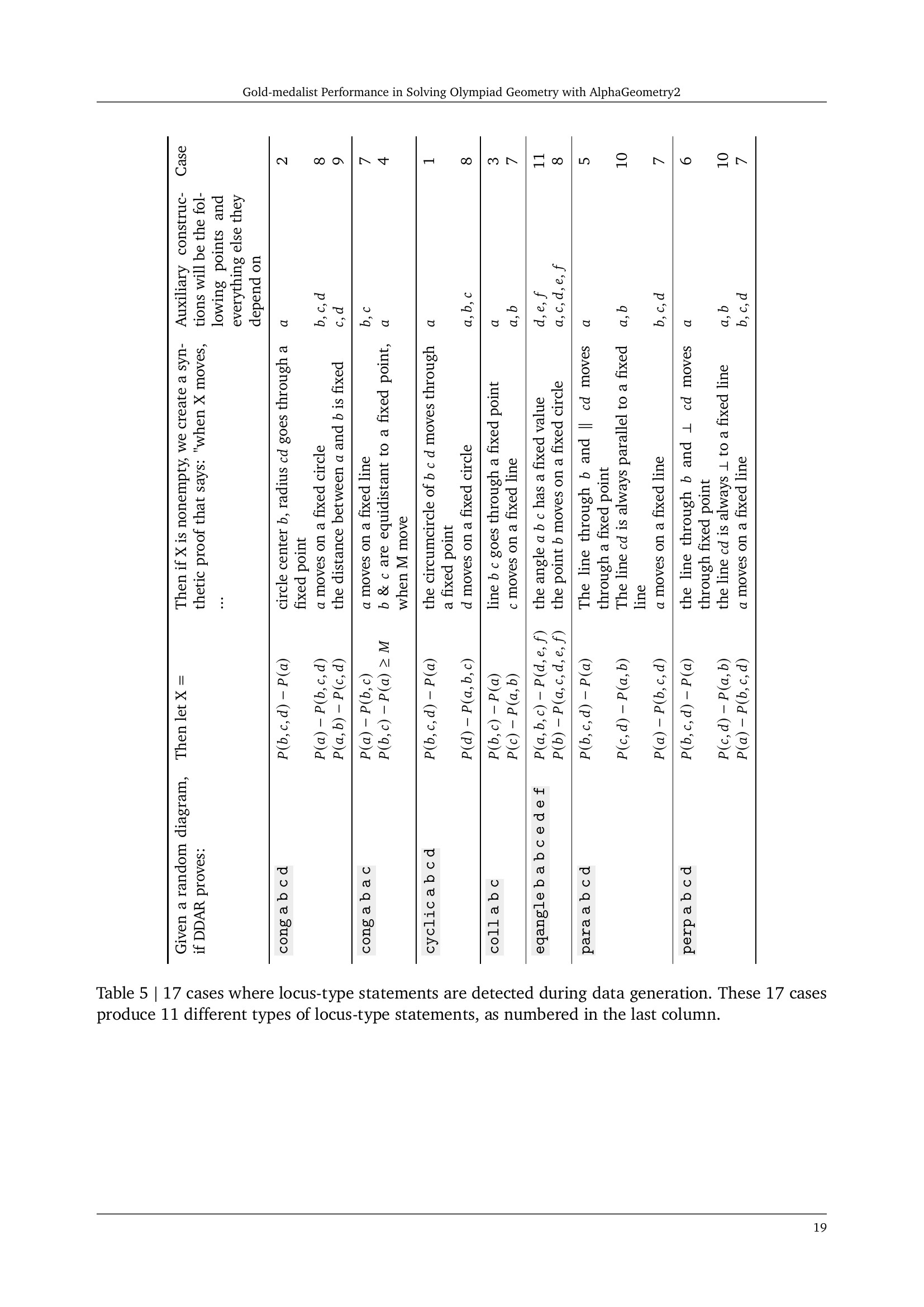
🔼 This table details 17 scenarios identified during the generation of synthetic training data where ’locus-type’ statements (describing the movement of geometric objects) were detected. Each scenario is described, along with the AlphaGeometry predicates used to represent it and the type of locus-type statement generated. Note that while there are 17 distinct scenarios, these scenarios result in only 11 unique types of locus statements. The table is organized to show the relationship between the initial conditions (input predicates) and the resulting locus-type statement generated by the system.
read the caption
Table 5: 17 cases where locus-type statements are detected during data generation. These 17 cases produce 11 different types of locus-type statements, as numbered in the last column.

TL;DR#

Key Takeaways#

Why does it matter?#

Visual Insights#

In-depth insights#

Neuro-Symbolic AI#

Gemini Language Model#

Automated Diagram Generation#

DDAR Enhancements#

Future Research#

More visual insights#

Full paper#