Scaling Laws in Patchification: An Image Is Worth 50,176 Tokens And More

2502.03738

Feng Wang et el.

🤗 2025-02-10

TL;DR
#

Vision Transformers (ViTs) typically use patchification, compressing images into smaller features. This study investigates information loss from this compression. Existing methods were computationally expensive due to quadratic scaling of self-attention and memory limitations, hindering comprehensive exploration.

This research conducts extensive experiments across different tasks and architectures by systematically reducing patch size. It surprisingly discovers a new scaling law: smaller patches consistently lead to improved accuracy until the minimum size (1x1, or pixel level). This applies broadly across tasks and models. Furthermore, it shows that smaller patches enable exceptional length sequences (50,176 tokens) achieving competitive results and reduce the dependence on decoder heads in dense prediction. This work fundamentally revisits visual encoding, suggesting potential for non-compressive models.

Key Takeaways
#

Why does it matter?
#

This paper challenges the conventional wisdom in vision transformer design by demonstrating the benefits of reducing patch size. It offers a novel scaling law, impacting various vision tasks and architectural designs. This opens up new avenues for research in efficient and high-performance visual models, potentially leading to breakthroughs in non-compressive vision.

Visual Insights
#

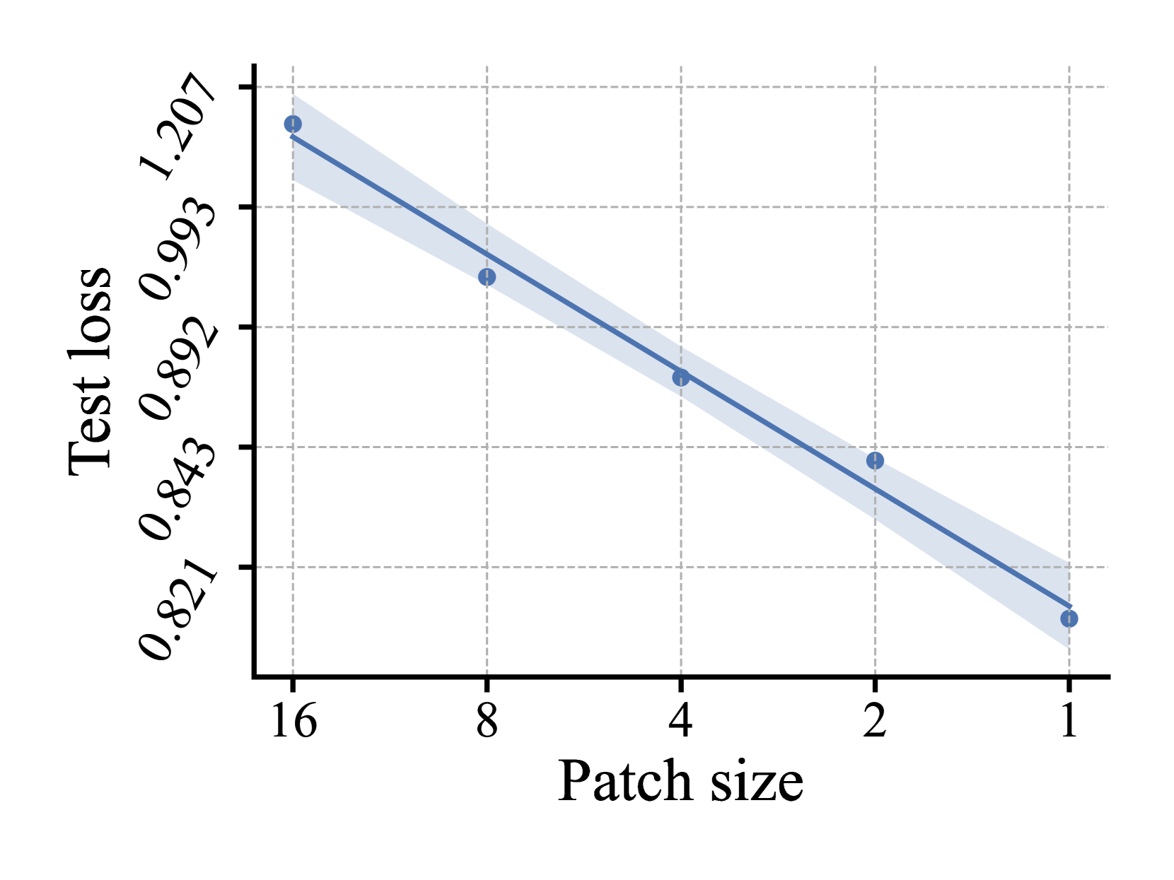
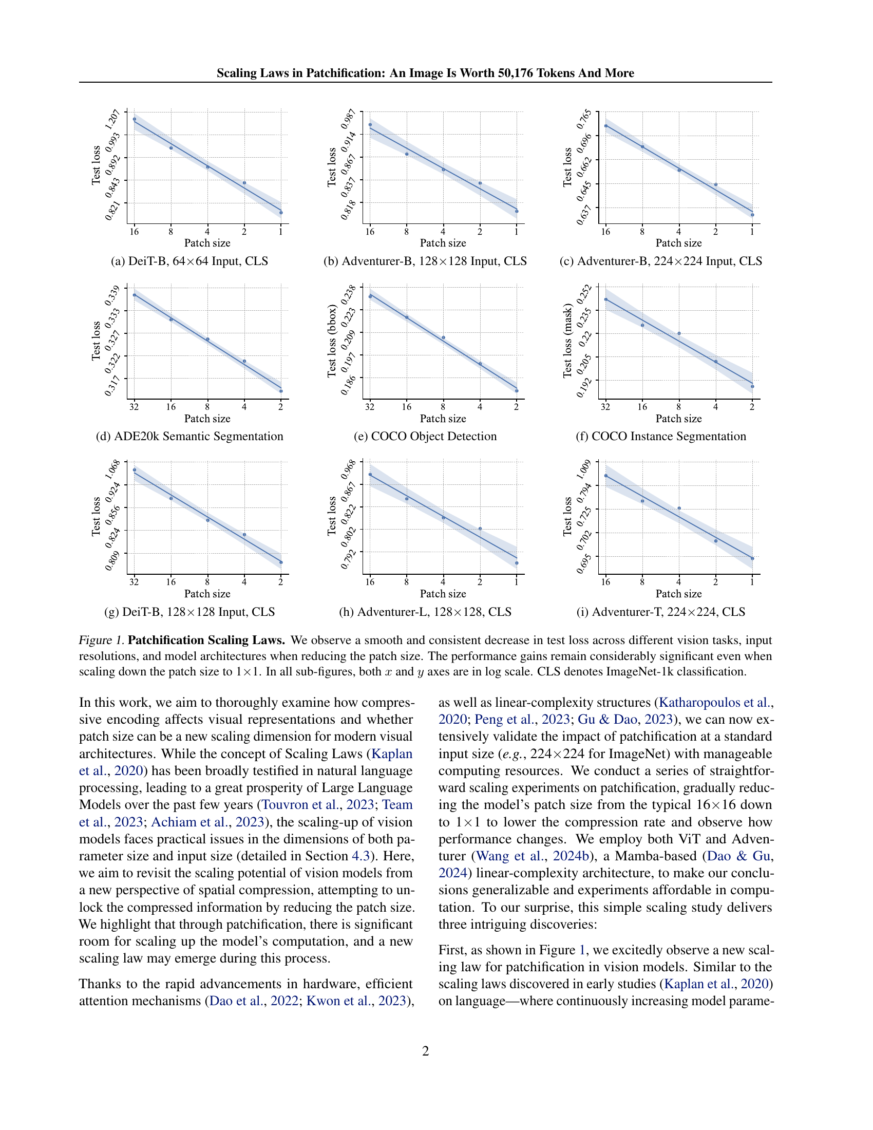
🔼 This figure shows the test loss results for DeiT-Base model with 64x64 input image size on the ImageNet-1k classification task. The x-axis represents the patch size used for image tokenization, ranging from 16 to 1. The y-axis shows the corresponding test loss. The plot demonstrates a clear trend where the test loss decreases as the patch size decreases, indicating that smaller patch sizes lead to improved performance.
read the caption
(a) DeiT-B, 64×\times×64 Input, CLS

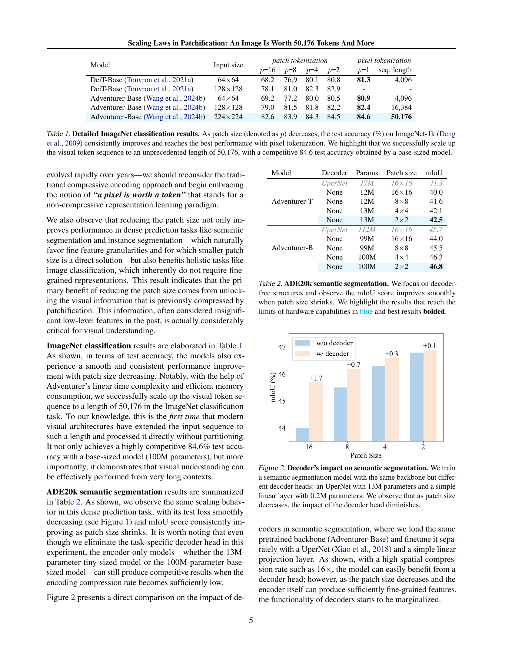
Model	Input size	patch tokenization				pixel tokenization
Model	Input size	$p$ =16	$p$ =8	$p$ =4	$p$ =2	$p$ =1	seq. length
DeiT-Base (Touvron et al., 2021a)	64 $\times$ 64	68.2	76.9	80.1	80.8	81.3	4,096
DeiT-Base (Touvron et al., 2021a)	128 $\times$ 128	78.1	81.0	82.3	82.9	-	-
Adventurer-Base (Wang et al., 2024b)	64 $\times$ 64	69.2	77.2	80.0	80.5	80.9	4,096
Adventurer-Base (Wang et al., 2024b)	128 $\times$ 128	79.0	81.5	81.8	82.2	82.4	16,384
Adventurer-Base (Wang et al., 2024b)	224 $\times$ 224	82.6	83.9	84.3	84.5	84.6	50,176

🔼 This table presents the ImageNet-1k classification accuracy for various models (DeiT-Base and Adventurer-Base) and patch sizes. The results demonstrate a consistent improvement in accuracy as the patch size decreases, culminating in the best performance with pixel tokenization (1x1 patch). Notably, the study successfully scales the visual sequence length to 50,176 tokens using a base-sized model (Adventurer-Base), achieving a competitive accuracy of 84.6%. The table showcases the impact of reducing patch size on accuracy for different input image sizes (64x64 and 128x128).
read the caption
Table 1: Detailed ImageNet classification results. As patch size (denoted as p𝑝pitalic_p) decreases, the test accuracy (%) on ImageNet-1k (Deng et al., 2009) consistently improves and reaches the best performance with pixel tokenization. We highlight that we successfully scale up the visual token sequence to an unprecedented length of 50,176, with a competitive 84.6 test accuracy obtained by a base-sized model.

In-depth insights
#

Patch Size Scaling Laws
#

The concept of “Patch Size Scaling Laws” in the context of Vision Transformers (ViTs) explores how altering the size of image patches before feeding them into the network affects model performance. The core finding is that reducing patch size consistently improves accuracy across various vision tasks and model architectures. This challenges the conventional wisdom of using larger patches (e.g., 16x16) for computational efficiency, demonstrating that the information loss from compression is detrimental. Smaller patches unlock more detailed visual information, leading to better results, even reaching the extreme of 1x1 (pixel-level) tokenization which outperforms patch-based methods. This suggests that the computational benefits of patchification can be outweighed by its limitations, particularly given the improvements in hardware. Importantly, smaller patches also diminish the importance of decoder components in dense prediction tasks, highlighting a potential shift towards encoder-only architectures for future visual models.

Vision Model Scaling
#

Vision model scaling explores strategies to enhance model performance by manipulating various dimensions. Increasing model size (parameter count) is a common approach, leading to improved accuracy but at the cost of significantly increased computational resources and potential overfitting. Data scaling, increasing the size of the training dataset, is another avenue, but obtaining high-quality, large datasets can be expensive and time-consuming. Resolution scaling, adjusting input image resolution, can impact performance, with higher resolutions providing more detail but also greater computational demands. A novel approach explored is patch size scaling, which systematically reduces the size of image patches fed into the model. This method surprisingly demonstrates consistent performance gains, even down to the level of pixel-level tokenization, unlocking potentially valuable information lost in traditional compressive methods. Sequence length scaling, increasing the number of tokens processed, is another aspect, where the tradeoffs between computational complexity and information density must be carefully considered. The interplay and relative effectiveness of these scaling dimensions are complex and depend on various factors including model architecture and task type. Finding the optimal balance between these dimensions is crucial for building efficient and high-performing vision models.

Decoder Head Impact
#

The research explores the impact of decoder heads in the context of patchification scaling. The study reveals that as patch sizes decrease, the reliance on decoder heads diminishes. This is attributed to the fact that smaller patches provide finer-grained visual information, reducing the need for a decoder to upsample and refine features. The results suggest a potential shift towards decoder-free architectures for dense prediction tasks, which could significantly simplify model design and improve efficiency. The findings challenge conventional wisdom, highlighting that the information loss due to patchification, while impactful, is not necessarily detrimental when appropriately addressed through scaling. This insight opens avenues for creating simpler, more computationally efficient vision models with competitive performance.

Long Sequence Encoding
#

The concept of “Long Sequence Encoding” in vision transformers is crucial for improving performance. Standard patchification methods, while efficient, inherently compress spatial information, potentially hindering model accuracy. Increasing the length of the input sequence, by reducing patch size to the extreme (pixel-level), allows the model to access a significantly richer representation of the input image. This approach, however, presents computational challenges. Efficient attention mechanisms and linear-complexity architectures are needed to manage the high dimensionality of long sequences. The tradeoff between computational cost and performance gains from extended sequences needs careful consideration. The paper’s exploration of scaling laws reveals that consistently improving model performance is achievable through decreasing patch size, until reaching pixel-level tokenization. This suggests a paradigm shift away from compressed encoding towards non-compressive approaches, maximizing the information available to the model. This paradigm change should be coupled with advancements in efficient computational methods to fully exploit the benefits of long-sequence encoding.

Future Research
#

Future research directions stemming from this paper on patchification scaling laws in vision transformers are exciting and multifaceted. Firstly, a deeper investigation into the theoretical underpinnings of the observed scaling laws is crucial. Why does reducing patch size consistently improve performance, even down to pixel-level tokenization? A more comprehensive theoretical model could unlock further advancements. Secondly, building upon the findings of this study, it’s essential to develop fully non-compressive vision models. The study’s success in achieving competitive results with exceptionally long token sequences suggests that the traditional patchification paradigm may be unnecessary. Thirdly, exploring the impact of this discovery on various downstream tasks beyond image classification, semantic segmentation, and object detection would yield significant insights. How would this approach affect tasks like video understanding or 3D scene analysis? Finally, investigating alternative, more efficient tokenization strategies in place of patchification warrants attention. The current focus could be expanded to explore other forms of image encoding that might enable even better scaling and performance. This multifaceted exploration could substantially advance visual representation learning and foundational visual model design.

More visual insights
#

More on figures

🔼 The figure shows the test loss for the Adventurer-B model with a 128x128 input image on the ImageNet-1k classification task. The x-axis represents different patch sizes used for image tokenization, and the y-axis shows the corresponding test loss. The plot demonstrates how the test loss varies as the patch size is changed, illustrating the effect of patch size on model performance for this specific model and task.
read the caption
(b) Adventurer-B, 128×\times×128 Input, CLS

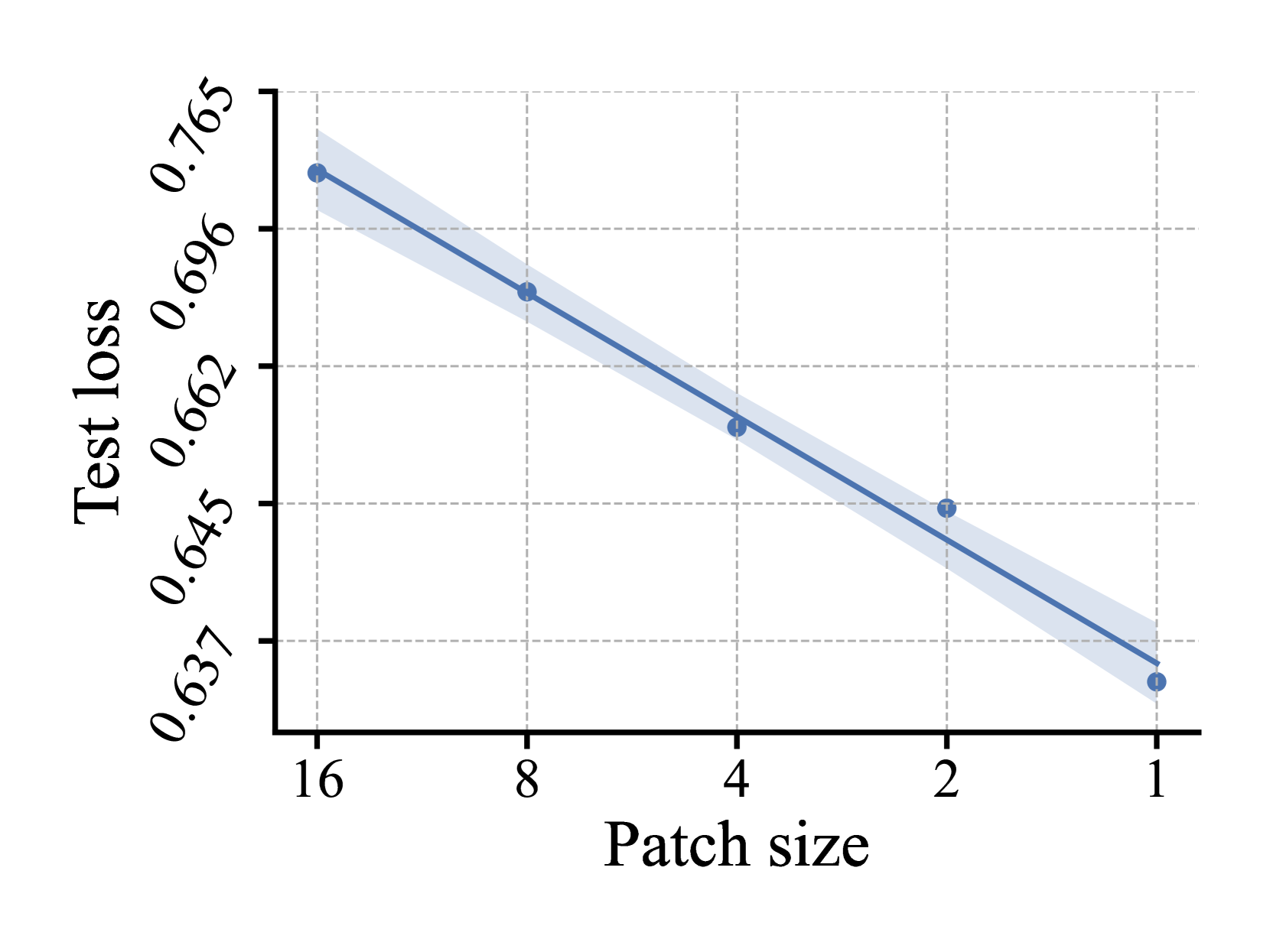
🔼 The figure shows the test loss for image classification on the ImageNet-1k dataset using the Adventurer-B model with a 224x224 input image and the classification head being the [CLS] token. It displays how the test loss changes as the patch size used in the patchification process is varied. The x-axis represents the patch size, and the y-axis represents the test loss. The plot demonstrates the relationship between patch size and model performance for this specific model and dataset.
read the caption
(c) Adventurer-B, 224×\times×224 Input, CLS

🔼 This figure shows the results of patch size scaling experiments on the ADE20k semantic segmentation dataset. It demonstrates how test loss changes as the patch size used for image tokenization decreases. The x-axis represents the patch size, and the y-axis represents the test loss. The graph visually depicts the scaling law observed in patchification, showing a consistent decrease in test loss as patch size decreases, indicating improved performance with smaller patches.
read the caption
(d) ADE20k Semantic Segmentation

🔼 This figure shows the test loss (in terms of bounding box) for COCO object detection across different patch sizes. The x-axis represents the patch size used for image tokenization, and the y-axis shows the corresponding test loss. The results demonstrate the impact of patch size on the performance of the object detection model. Smaller patch sizes generally lead to lower test loss, indicating improved performance.
read the caption
(e) COCO Object Detection

🔼 This figure shows the test loss (mask) for COCO instance segmentation plotted against patch size. The graph displays the impact of varying patch sizes on the model’s performance for this specific task. The results are presented in log scale for both the x and y axes.
read the caption
(f) COCO Instance Segmentation

🔼 This figure shows the test loss for different patch sizes when training a DeiT-Base model on the ImageNet-1k classification task. The input image size is 128x128 pixels, and the classification is performed using the CLS token. The x-axis represents the patch size (on a log scale), and the y-axis represents the test loss (also on a log scale). The figure demonstrates the impact of reducing patch size on model performance.
read the caption
(g) DeiT-B, 128×\times×128 Input, CLS

🔼 This figure shows the test loss for the Adventurer-Large model with a 128x128 input image on the ImageNet-1k classification task (CLS). The x-axis represents the patch size used for image tokenization, and the y-axis represents the test loss. The plot demonstrates how test loss changes as the patch size decreases, illustrating the impact of patch size on model performance. This plot shows that consistently decreasing the patch size improves the performance, reaching the minimum at 1x1(pixel tokenization).
read the caption
(h) Adventurer-L, 128×\times×128, CLS

🔼 This figure displays the results of patch size scaling experiments conducted on the Adventurer-T model with a 224x224 input image for ImageNet-1k classification (CLS). It visually represents how the model’s test loss changes as the patch size decreases, demonstrating the impact of patch size on model performance.
read the caption
(i) Adventurer-T, 224×\times×224, CLS

🔼 This figure visualizes the impact of patch size on the performance of various vision models across different tasks. The x-axis represents the patch size (on a logarithmic scale), while the y-axis shows the test loss (also on a logarithmic scale). The plots demonstrate a consistent trend: as the patch size decreases, the test loss decreases, indicating improved model performance. This trend is observed across various vision tasks (classification, semantic segmentation, object detection, and instance segmentation), input resolutions, and model architectures (DeiT and Adventurer). Even when the patch size is reduced to the minimum of 1x1 (pixel-level processing), significant performance gains are maintained. The ImageNet-1k classification task is specifically highlighted using the abbreviation ‘CLS’.
read the caption
Figure 1: Patchification Scaling Laws. We observe a smooth and consistent decrease in test loss across different vision tasks, input resolutions, and model architectures when reducing the patch size. The performance gains remain considerably significant even when scaling down the patch size to 1×\times×1. In all sub-figures, both x𝑥xitalic_x and y𝑦yitalic_y axes are in log scale. CLS denotes ImageNet-1k classification.

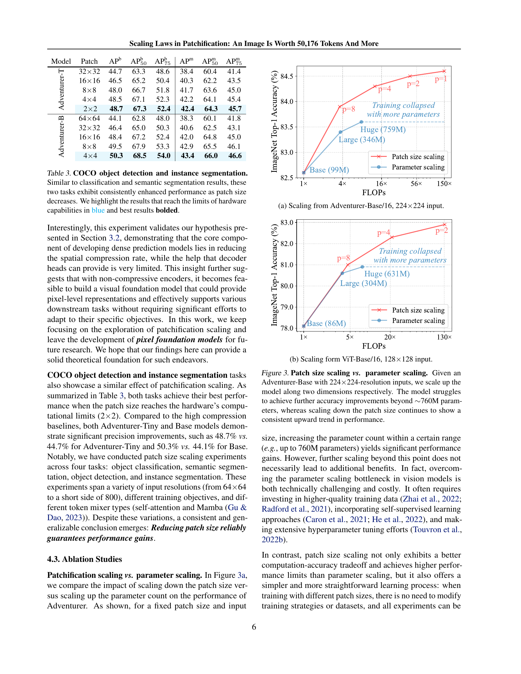
🔼 This figure compares the performance of semantic segmentation models using two different decoder heads: a complex UperNet with 13 million parameters and a simple linear layer with only 0.2 million parameters. Both models share the same backbone network. The x-axis represents the patch size used in the model, showing the results as the patch size decreases from 16x16 to 2x2. The y-axis represents the mean Intersection over Union (mIoU), a common metric for evaluating semantic segmentation accuracy. The results demonstrate that as the patch size decreases, the performance difference between the two decoder types diminishes, suggesting that the complex decoder becomes less crucial when using smaller patch sizes and the resulting increased level of detail. This implies that the additional complexity of the UperNet offers diminishing returns as the input’s spatial resolution increases.
read the caption
Figure 2: Decoder’s impact on semantic segmentation. We train a semantic segmentation model with the same backbone but different decoder heads: an UperNet with 13M parameters and a simple linear layer with 0.2M parameters. We observe that as patch size decreases, the impact of the decoder head diminishes.

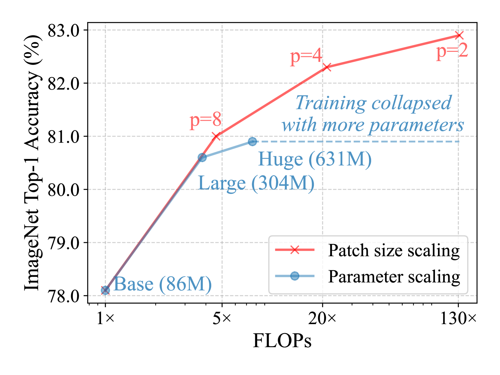
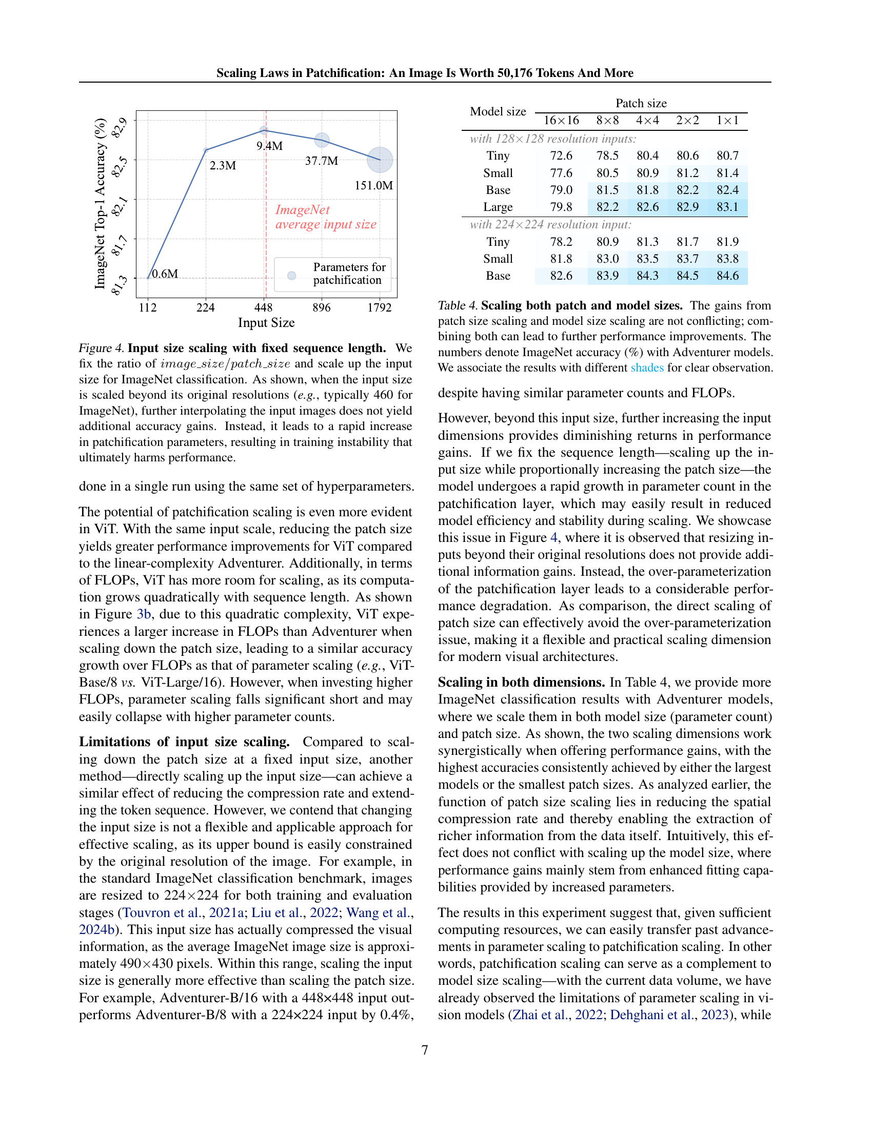
🔼 This figure compares the impact of increasing model parameters versus reducing patch size on the performance of the Adventurer model for ImageNet classification. The x-axis represents FLOPS (floating point operations per second), a measure of computational cost. The y-axis represents ImageNet top-1 accuracy. Different colored lines represent models with varying parameter counts, showing the impact of simply increasing model size. The lines with different patch sizes show how reducing the patch size (and therefore increasing the sequence length) impacts accuracy while controlling for model size. The figure demonstrates that reducing patch size consistently improves accuracy more effectively than increasing model size beyond a certain point.
read the caption
(a) Scaling from Adventurer-Base/16, 224×\times×224 input.

🔼 This figure compares the impact of increasing model parameters versus decreasing patch size on the performance of a ViT-Base model with a 128x128 input image. The x-axis represents FLOPs (floating-point operations), a measure of computational cost, and the y-axis represents ImageNet top-1 accuracy. It shows that increasing model parameters leads to diminishing returns in accuracy after a certain point, while reducing patch size consistently improves accuracy.
read the caption
(b) Scaling form ViT-Base/16, 128×\times×128 input.

More on tables

Model	Decoder	Params	Patch size	mIoU
Adventurer-T	UperNet	17M	16 $\times$ 16	41.3
	None	12M	16 $\times$ 16	40.0
	None	12M	8 $\times$ 8	41.6
	None	13M	4 $\times$ 4	42.1
	None	13M	2 $\times$ 2	42.5
Adventurer-B	UperNet	112M	16 $\times$ 16	45.7
	None	99M	16 $\times$ 16	44.0
	None	99M	8 $\times$ 8	45.5
	None	100M	4 $\times$ 4	46.3
	None	100M	2 $\times$ 2	46.8

🔼 This table presents the results of ADE20K semantic segmentation experiments using decoder-free architectures. It shows how the mean Intersection over Union (mIoU) score changes as the patch size used in the model is reduced. The experiment focuses on exploring the effect of patch size without a decoder, demonstrating performance gains as the patch size decreases. Results are presented for different model sizes (parameter counts), highlighting those that reached the computational limits of the hardware used in the experiment. The best results for each model size are shown in bold. Results that approach the limits of hardware capabilities are shown in blue.
read the caption
Table 2: ADE20k semantic segmentation. We focus on decoder-free structures and observe the mIoU score improves smoothly when patch size shrinks. We highlight the results that reach the limits of hardware capabilities in blue and best results bolded.

Model	Patch	AP ${}^{\text{b}}$	AP ${}^{\text{b}}_{50}$	AP ${}^{\text{b}}_{75}$	AP ${}^{\text{m}}$	AP ${}^{\text{m}}_{50}$	AP ${}^{\text{m}}_{75}$
Adventurer-T	32 $\times$ 32	44.7	63.3	48.6	38.4	60.4	41.4
	16 $\times$ 16	46.5	65.2	50.4	40.3	62.2	43.5
	8 $\times$ 8	48.0	66.7	51.8	41.7	63.6	45.0
	4 $\times$ 4	48.5	67.1	52.3	42.2	64.1	45.4
	2 $\times$ 2	48.7	67.3	52.4	42.4	64.3	45.7
Adventurer-B	64 $\times$ 64	44.1	62.8	48.0	38.3	60.1	41.8
	32 $\times$ 32	46.4	65.0	50.3	40.6	62.5	43.1
	16 $\times$ 16	48.4	67.2	52.4	42.0	64.8	45.0
	8 $\times$ 8	49.5	67.9	53.3	42.9	65.5	46.1
	4 $\times$ 4	50.3	68.5	54.0	43.4	66.0	46.6

🔼 Table 3 presents the results of COCO object detection and instance segmentation experiments. It shows the Average Precision (AP) at different Intersection over Union (IoU) thresholds (AP50, AP75, AP) and average precision across all thresholds (AP) for both Adventurer-B and Adventurer-T models using various patch sizes. As the patch size decreases, the performance consistently improves across all metrics, demonstrating the effectiveness of reducing the patch size in object detection and instance segmentation tasks. The best performing results (those limited by hardware capabilities) are highlighted in blue, and the overall best results for each model are bolded.
read the caption
Table 3: COCO object detection and instance segmentation. Similar to classification and semantic segmentation results, these two tasks exhibit consistently enhanced performance as patch size decreases. We highlight the results that reach the limits of hardware capabilities in blue and best results bolded.

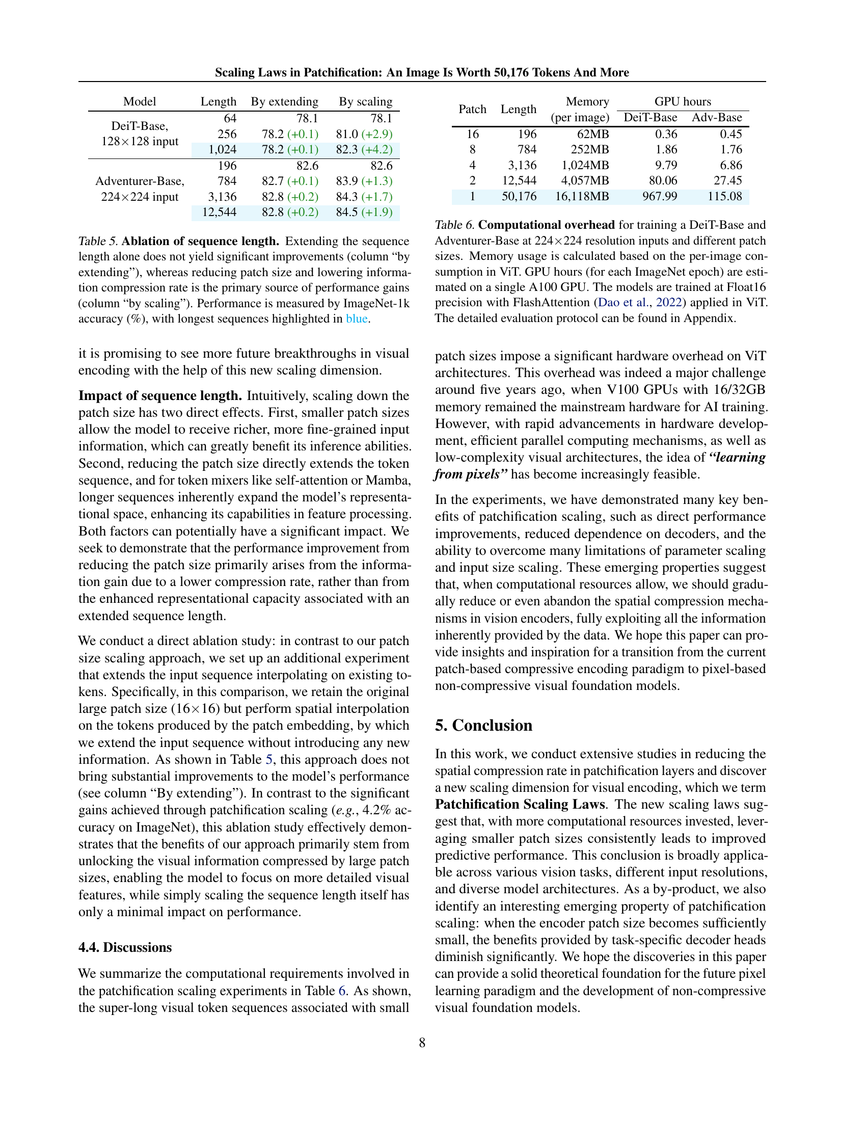
Model size	Patch size
Model size	16 $\times$ 16	8 $\times$ 8	4 $\times$ 4	2 $\times$ 2	1 $\times$ 1
with 128 $\times$ 128 resolution inputs:
Tiny	72.6	78.5	80.4	80.6	80.7
Small	77.6	80.5	80.9	81.2	81.4
Base	79.0	81.5	81.8	82.2	82.4
Large	79.8	82.2	82.6	82.9	83.1
with 224 $\times$ 224 resolution input:
Tiny	78.2	80.9	81.3	81.7	81.9
Small	81.8	83.0	83.5	83.7	83.8
Base	82.6	83.9	84.3	84.5	84.6

🔼 This table presents ImageNet-1k classification accuracy results (%) for Adventurer models of various sizes (Tiny, Small, Base, Large) and patch sizes (16x16, 8x8, 4x4, 2x2, 1x1). It demonstrates that improvements from increasing model size and decreasing patch size are not mutually exclusive; rather, combining both approaches leads to even higher accuracy. Different shades are used to visually highlight the relationship between model size, patch size, and accuracy.
read the caption
Table 4: Scaling both patch and model sizes. The gains from patch size scaling and model size scaling are not conflicting; combining both can lead to further performance improvements. The numbers denote ImageNet accuracy (%) with Adventurer models. We associate the results with different shades for clear observation.

Model	Length	By extending	By scaling
DeiT-Base,	64	78.1	78.1
128 $\times$ 128 input	256	78.2 (+0.1)	81.0 (+2.9)
128 $\times$ 128 input	1,024	78.2 (+0.1)	82.3 (+4.2)
	196	82.6	82.6
Adventurer-Base,	784	82.7 (+0.1)	83.9 (+1.3)
224 $\times$ 224 input	3,136	82.8 (+0.2)	84.3 (+1.7)
	12,544	82.8 (+0.2)	84.5 (+1.9)

🔼 This table investigates the impact of sequence length on model performance by comparing two methods: extending the sequence length while keeping the patch size constant and reducing the patch size to lower the information compression rate. The results show that reducing the patch size leads to significant performance gains, while simply extending the sequence length yields minimal improvement. The primary performance improvements come from the reduced information compression rate rather than the increased sequence length. ImageNet-1k accuracy is used to measure performance, highlighting the best results achieved with longer sequences in blue.
read the caption
Table 5: Ablation of sequence length. Extending the sequence length alone does not yield significant improvements (column “by extending”), whereas reducing patch size and lowering information compression rate is the primary source of performance gains (column “by scaling”). Performance is measured by ImageNet-1k accuracy (%), with longest sequences highlighted in blue.

Patch	Length	Memory	GPU hours
Patch	Length	(per image)	DeiT-Base	Adv-Base
16	196	62MB	0.36	0.45
8	784	252MB	1.86	1.76
4	3,136	1,024MB	9.79	6.86
2	12,544	4,057MB	80.06	27.45
1	50,176	16,118MB	967.99	115.08

🔼 This table details the computational resources required to train DeiT-Base and Adventurer-Base vision transformer models on ImageNet at a 224x224 resolution, using varying patch sizes. The memory consumption per image is shown, and the GPU hours needed per ImageNet epoch are estimated using a single A100 GPU. The models were trained with Float16 precision and FlashAttention (Dao et al., 2022) for DeiT. Further training details are available in the Appendix.
read the caption
Table 6: Computational overhead for training a DeiT-Base and Adventurer-Base at 224×\times×224 resolution inputs and different patch sizes. Memory usage is calculated based on the per-image consumption in ViT. GPU hours (for each ImageNet epoch) are estimated on a single A100 GPU. The models are trained at Float16 precision with FlashAttention (Dao et al., 2022) applied in ViT. The detailed evaluation protocol can be found in Appendix.

Model	Embedding dimension	MLP dimension	Blocks	Parameters
DeiT-Tiny (Touvron et al., 2021a)	192	768	12	5M
DeiT-Small (Touvron et al., 2021a)	384	1,536	12	22M
DeiT-Base (Touvron et al., 2021a)	768	3,072	12	86M
DeiT-Large (Touvron et al., 2022b)	1,024	4,096	24	304M
DeiT-Huge (Touvron et al., 2022b)	1,280	5,120	32	631M
Adventurer-Tiny (Wang et al., 2024b)	256	640	12	12M
Adventurer-Small (Wang et al., 2024b)	512	1,280	12	44M
Adventurer-Base (Wang et al., 2024b)	768	1,920	12	99M
Adventurer-Large (Wang et al., 2024b)	1,024	2,560	24	346M
Adventurer-Huge (Wang et al., 2024b)	1,280	3,200	32	759M

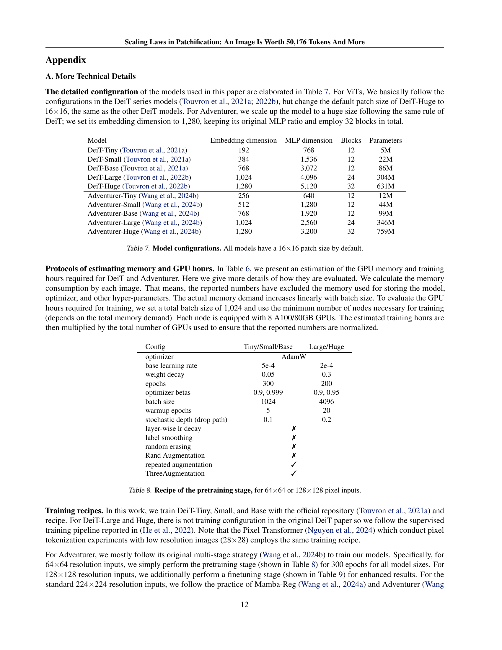
🔼 This table details the configurations used for different vision transformer models in the experiments. It shows the embedding dimension, MLP (Multilayer Perceptron) dimension, number of blocks in the architecture, and the total number of parameters for each model variant (Tiny, Small, Base, Large, Huge). Note that all models listed here initially use a 16x16 patch size.
read the caption
Table 7: Model configurations. All models have a 16×\times×16 patch size by default.

Config	Tiny/Small/Base	Large/Huge
optimizer	AdamW
base learning rate	5e-4	2e-4
weight decay	0.05	0.3
epochs	300	200
optimizer betas	0.9, 0.999	0.9, 0.95
batch size	1024	4096
warmup epochs	5	20
stochastic depth (drop path)	0.1	0.2
layer-wise lr decay	✗
label smoothing	✗
random erasing	✗
Rand Augmentation	✗
repeated augmentation	✓
ThreeAugmentation	✓

🔼 Table 8 presents the hyperparameters used during the pretraining phase of the vision transformer models. It details the configuration for both the DeiT and Adventurer model architectures, specifying settings such as the optimizer (AdamW), base learning rate, weight decay, number of epochs, and various data augmentation techniques (random erasing, RandAugment, etc.). The table highlights the differences in hyperparameters between smaller (Tiny/Small/Base) and larger (Large/Huge) models, reflecting the scaling strategies employed in the experiments. The table shows that different hyperparameter settings were used to train the models with 64x64 and 128x128 pixel inputs.
read the caption
Table 8: Recipe of the pretraining stage, for 64×\times×64 or 128×\times×128 pixel inputs.

Config	Small/Base	Large
optimizer	AdamW
base learning rate	1e-5	2e-5
weight decay	0.1	0.1
epochs	20	50
optimizer betas	0.9, 0.999	0.9, 0.95
batch size	512	512
warmup epochs	5	5
stochastic depth (drop path)	0.4 (S), 0.6 (B)	0.6
layer-wise lr decay	✗	0.95
label smoothing	0.1
random erasing	✗
Rand Augmentation	rand-m9-mstd0.5-inc1
repeated augmentation	✗
ThreeAugmentation	✗

🔼 This table details the hyperparameters used in the finetuning stage of the training process for the Adventurer models. Finetuning is performed after an initial pretraining stage (see Table 8). The table shows configurations for different model sizes (Small and Base) and input resolutions (128x128 and 224x224 pixels). Hyperparameters shown include the optimizer, learning rate, weight decay, number of epochs, beta parameters for the optimizer, batch size, warmup epochs, stochastic depth, layer-wise learning rate decay, label smoothing, random erasing, and augmentation techniques used.
read the caption
Table 9: Recipe of the finetuning stage, for 128×\times×128 or 224×\times×224 pixel inputs.

Config	Small/Base	Large
optimizer	AdamW
base learning rate	5e-4	8e-4
weight decay	0.05	0.3
epochs	100	50
optimizer betas	0.9, 0.999	0.9, 0.95
batch size	1024	4096
warmup epochs	5	20
stochastic depth (drop path)	0.2 (S), 0.4 (B)	0.4
layer-wise lr decay	✗	0.9
label smoothing	✗
random erasing	✗
Rand Augmentation	✗
repeated augmentation	✓
ThreeAugmentation	✓

🔼 Table 10 details the hyperparameters used in the intermediate training stage for the Adventurer model when using 224x224 pixel inputs. It shows the optimizer used (AdamW), learning rate, weight decay, number of epochs, beta values for the optimizer, batch size, warm-up epochs, stochastic depth, layer-wise learning rate decay, label smoothing, random erasing, and data augmentation techniques (RandAugmentation, Repeated Augmentation, ThreeAugmentation). The table provides separate configurations for smaller (Small/Base) and larger (Large) versions of the Adventurer model, indicating different hyperparameter settings depending on model size.
read the caption
Table 10: Recipe of the intermediate training stage, for 224×\times×224 pixel inputs.

TL;DR#

Key Takeaways#

Why does it matter?#

Visual Insights#

In-depth insights#

Patch Size Scaling Laws#

Vision Model Scaling#

Decoder Head Impact#

Long Sequence Encoding#

Future Research#

More visual insights#

Full paper#