TL;DR#
Multimodal understanding and generation models struggle with visual tokenization, needing a separate tokenizer for each task. This often results in a trade-off between good reconstruction quality and semantic understanding. Existing methods struggle to balance the requirements of contrastive learning (for alignment) and reconstruction objectives, often requiring high memory and large batch sizes.
QLIP tackles this problem by introducing a novel visual tokenization method that effectively combines both objectives. It employs a two-stage training process to address the memory bottleneck and uses dynamic loss weighting to balance reconstruction and alignment. QLIP achieves state-of-the-art performance on both image reconstruction and zero-shot image understanding, demonstrating its efficacy as a drop-in replacement for visual encoders in existing multimodal models. The proposed method also shows the promise of a unified model for multimodal tasks.
Key Takeaways#
Why does it matter?#
This paper is important because it introduces QLIP, a novel visual tokenization method that significantly improves both the image reconstruction quality and zero-shot image understanding capabilities. This addresses a major challenge in multimodal learning, where the existing trade-off between these two crucial aspects has limited the performance of autoregressive models. QLIP’s unified approach paves the way for more efficient and effective multimodal models for understanding and generation tasks, opening up new avenues for research and development.
Visual Insights#

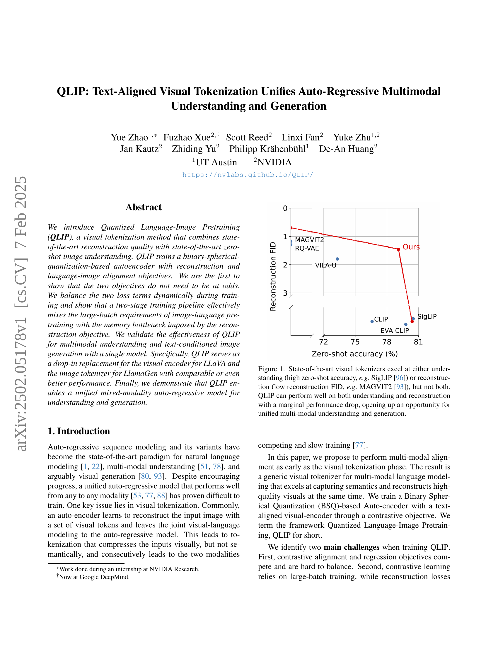
🔼 The figure illustrates the trade-off between zero-shot image classification accuracy and reconstruction quality (measured by FID) in state-of-the-art visual tokenizers. Existing methods like SigLIP prioritize accuracy, achieving high scores in zero-shot tasks but poor reconstruction quality; methods like MAGVIT2 prioritize reconstruction, showing low FID but poor accuracy in zero-shot settings. In contrast, QLIP achieves a balance between these two objectives, demonstrating strong performance in both zero-shot classification and image reconstruction, with only a minor decrease in performance compared to the best-performing models in each category. This balance allows QLIP to be used in a unified multimodal framework for both understanding and generation tasks.
read the caption
Figure 1: State-of-the-art visual tokenizers excel at either understanding (high zero-shot accuracy, e.g. SigLIP [96]) or reconstruction (low reconstruction FID, e.g. MAGVIT2 [93]), but not both. QLIP can perform well on both understanding and reconstruction with a marginal performance drop, opening up an opportunity for unified multi-modal understanding and generation.
| Dataset | Images | Text (# tok/src) | Usage/Metrics |
|---|---|---|---|
| DataComp-1B [27] | 1B | 20B/alt-text | QLIP |
| LAION-COCO [67]222hf.co/datasets/guangyil/laion-coco-aesthetic | 4M/600M | 40M/BLIP2 | T2I (LlamaGen), UM3 |
| SA-1B [41] | 11M | 400M/Qwen2VL-7B | T2I (LlamaGen), UM3 |
| CC-12M [9] | 6M/12M | 200M/Qwen2VL-7B | UM3 |
| DCLM [45] | - | 300B/raw+filtered | UM3 |
| LAION-CC-SBU [51] | 558K | -/BLIP2 | VLM (LLaVA-1.5) |
| LLaVA-Instruct [51] | 665K | -/convo. | VLM (LLaVA-1.5) |
| ImageNet [20] | 1.3M | -/label | Classi. (ZS), Recon. (RC) |
| MS-COCO [48, 11] | 160K | 10M/MTurk | Caption, generation |
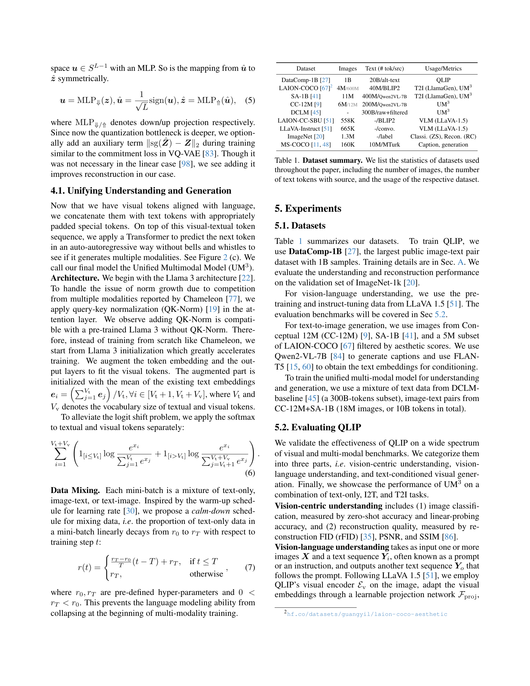
🔼 This table provides a comprehensive overview of the datasets utilized in the research paper. It details the name of each dataset, the quantity of images and text tokens (including the source of the text), and the specific tasks or metrics for which each dataset was employed in the experiments. This information is crucial for understanding the scope and methodology of the research.
read the caption
Table 1: Dataset summary. We list the statistics of datasets used throughout the paper, including the number of images, the number of text tokens with source, and the usage of the respective dataset.
In-depth insights#
Visual Tokenization#
Visual tokenization, a crucial aspect of multimodal learning, aims to bridge the gap between raw visual data and the discrete representations needed for auto-regressive models. The core challenge lies in creating a tokenization scheme that effectively captures both visual information and semantic meaning. Early methods focused primarily on reconstruction quality, using techniques like VQ-VAE, but these often sacrificed semantic richness. The paper highlights that a balance between reconstruction and semantic alignment is key; a purely reconstruction-focused approach leads to visually compressed but semantically poor tokens, hindering multimodal understanding. This is addressed by employing a contrastive learning approach integrated with the auto-encoder, aligning visual tokens with textual descriptions. This dual-objective training, although challenging due to differing gradient magnitudes and memory constraints, is shown to create tokens effective for both understanding and generation tasks. The innovative two-stage training process mitigates these challenges, enhancing both reconstruction and alignment capabilities. Overall, the discussion underscores the critical role of text alignment in visual tokenization, moving beyond simple reconstruction towards semantically meaningful representations for unified multimodal understanding and generation.
Two-Stage Training#
The authors cleverly address the challenge of balancing competing objectives and memory constraints in training their QLIP model through a two-stage training strategy. Stage one prioritizes semantic alignment using contrastive learning alongside MSE loss, leveraging a memory-efficient Transformer architecture to accommodate large batch sizes essential for contrastive learning. This stage efficiently establishes strong visual-textual relationships. Stage two, however, focuses on refining visual reconstruction quality. By freezing the visual encoder and dropping the contrastive loss, the authors enable smaller batch sizes for the reconstruction objective which is memory intensive, allowing for the optimization of perceptual and GAN losses to boost the visual fidelity. This two-stage approach is highly effective because it decouples the contrasting requirements of semantic alignment and visual reconstruction, enabling the model to successfully achieve both high-quality reconstruction and state-of-the-art zero-shot performance. The dynamic loss weighting further enhances this process, ensuring balanced optimization and mitigating potential issues arising from differences in gradient magnitude between the objectives.
Multimodal Model#
The concept of a multimodal model, capable of understanding and generating content across various modalities like text and images, is a central theme. The research explores the challenges in creating such a model, particularly concerning visual tokenization. Visual tokenization, the process of converting images into discrete tokens for processing by an autoregressive model, is highlighted as a crucial area. The authors introduce QLIP (Quantized Language-Image Pretraining), a novel visual tokenization method that aims to bridge the gap between high reconstruction quality and zero-shot image understanding performance. By dynamically balancing the reconstruction and alignment objectives during training, QLIP learns visual tokens that are not only visually representative but also semantically meaningful. This allows for integration with auto-regressive models, creating a unified architecture for both understanding and generation. The two-stage training approach, addressing memory constraints and balancing the objectives, is a key innovation. The results demonstrate QLIP’s effectiveness as a drop-in replacement for existing visual encoders in state-of-the-art multimodal models, achieving comparable or even better performance. The development of a unified multimodal model architecture is a major advance, enabling a single model to handle diverse tasks, further highlighting the potential of QLIP for future multimodal applications.
Ablation Studies#
Ablation studies systematically assess the contribution of individual components within a model. In this research, ablation experiments were conducted to isolate and understand the impact of specific design choices. The results likely revealed the relative importance of each component for achieving optimal performance. For example, analyzing the effect of different loss functions (e.g. reconstruction, alignment) and their weighting would show which objective is most crucial. Balancing these objectives is critical since a disproportionate focus on one might hinder the other. The two-stage training strategy was probably investigated to determine if its separation of objectives improved overall results or if a single-stage training method sufficed. This is important because multi-stage training is often more computationally intensive. Initializing the visual encoder from pre-trained models (e.g., MIM, CLIP) was likely compared to random initialization to gauge the impact of transfer learning on efficiency and performance. Analyzing the impact of the quantizer on both reconstruction and understanding is key. Overall, the ablation studies likely provide strong evidence to support the design choices made in the main model, demonstrating the effectiveness of each feature and identifying potential areas for further improvement.
Future of QLIP#
The future of QLIP (Quantized Language-Image Pretraining) looks promising, given its demonstrated ability to unify auto-regressive multimodal understanding and generation. Further research could focus on scaling QLIP to even larger datasets and model sizes, potentially leveraging techniques like model parallelism and more efficient training strategies. Improving the efficiency of the two-stage training process is another key area, perhaps through exploring alternative loss weighting schemes or novel training architectures. Investigating the impact of different quantization methods beyond BSQ could lead to further improvements in reconstruction quality and computational efficiency. Exploring the application of QLIP to other modalities, such as audio and video, would significantly broaden its capabilities and impact. Finally, deeper integration with existing large language models and more extensive benchmarking across a wider variety of tasks are crucial steps to solidify QLIP’s position as a leading multimodal architecture.
More visual insights#
More on figures

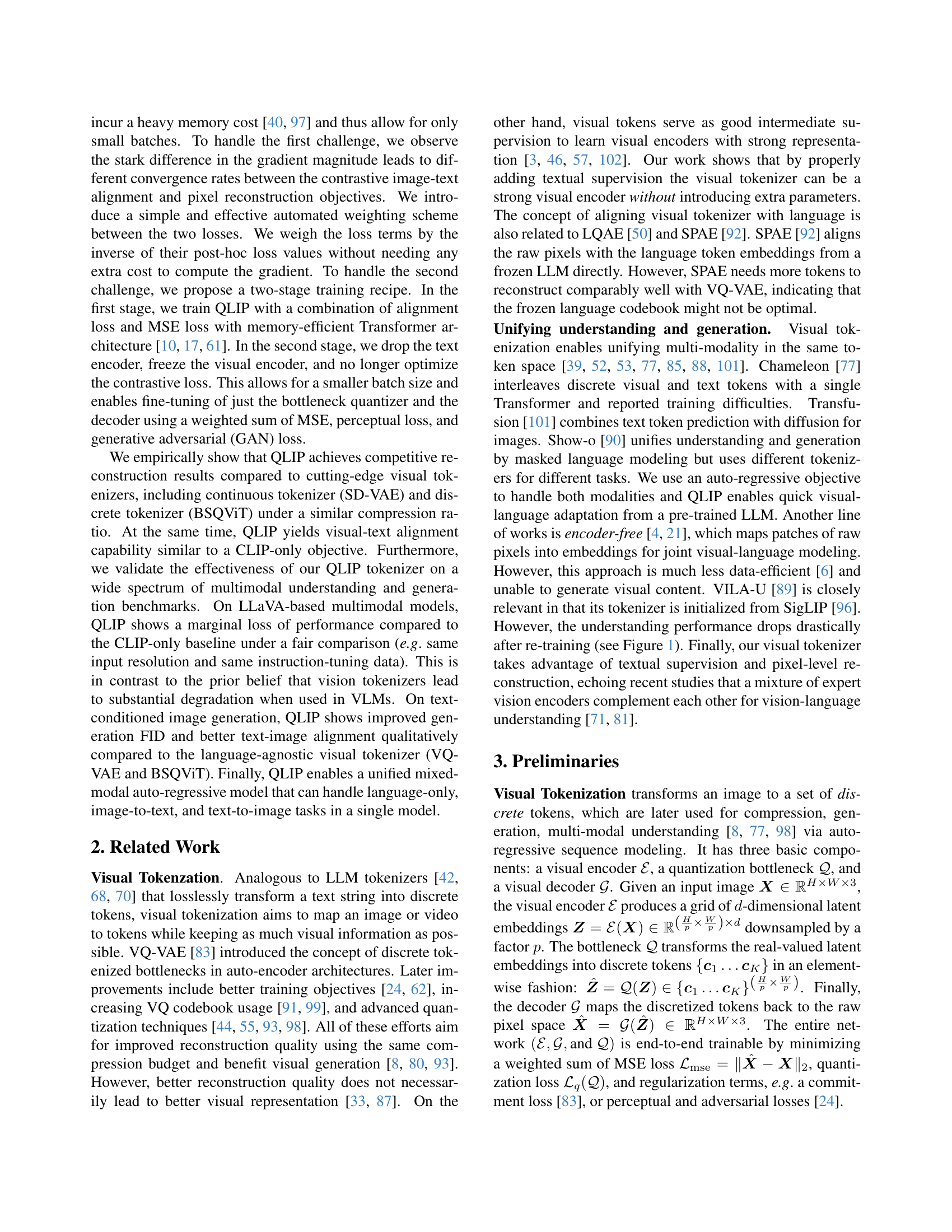
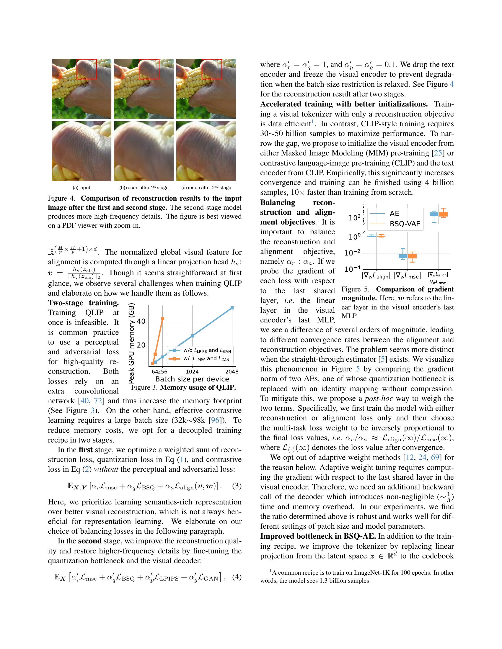
🔼 Figure 2 illustrates the QLIP model training and its application. (a) and (b) detail the two-stage training process. Stage 1 involves simultaneous training of image-text alignment and image reconstruction, while stage 2 focuses solely on enhancing reconstruction quality by fine-tuning specific components after freezing the visual encoder. (c) shows how a text-aligned visual tokenizer processes images into visual tokens for integration with text tokens within a unified multimodal autoregressive model, enabling joint modeling of both modalities.
read the caption
Figure 2: Overview. (a-b) Two-stage training pipeline of QLIP. (a) In Stage 1, we train QLIP with a combination of alignment loss and MSE loss. (b) In Stage 2, we drop the text encoder, freeze the visual encoder, and no longer optimize the contrastive loss. Only the bottleneck quantizer and the decoder are fine-tuned. (c) With the text-aligned visual tokenizer, we transform the image into visual tokens, concatenate them with text tokens, and use an auto-regressive multi-modal model (Sec 4.1) to model jointly.

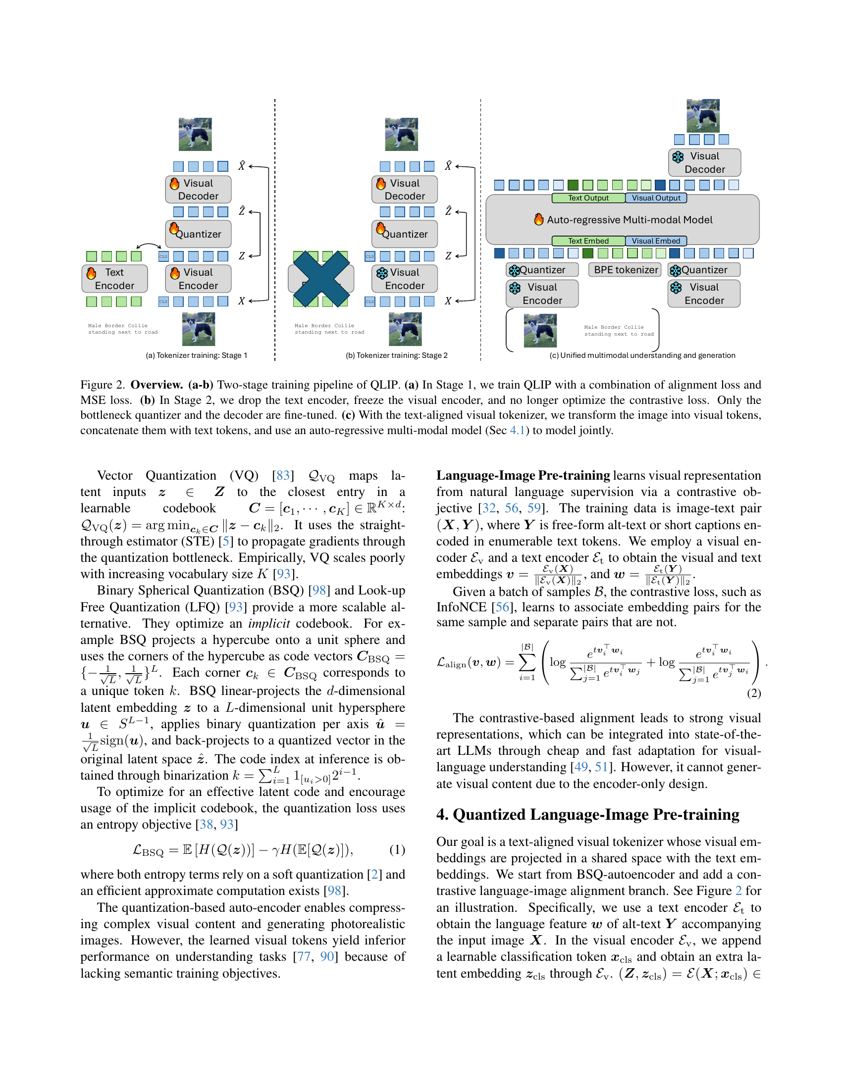
🔼 This figure shows a plot illustrating the GPU memory usage of the Quantized Language-Image Pretraining (QLIP) model during training. The x-axis represents the batch size used per device, while the y-axis shows the peak GPU memory consumption in gigabytes. Two lines are shown, one for training QLIP without the Learned Perceptual Image Patch Similarity (LPIPS) and Generative Adversarial Network (GAN) losses, and another for training with these losses included. The plot demonstrates the significant increase in memory usage when incorporating LPIPS and GAN losses, highlighting a key challenge addressed by the two-stage training strategy employed in the QLIP method.
read the caption
Figure 3: Memory usage of QLIP.

🔼 This figure displays a comparison of image reconstruction results at different stages of the QLIP training process. The leftmost column shows the original input image. The middle column shows the reconstruction after the first training stage, which primarily focuses on contrastive language-image alignment and MSE loss for reconstruction. The rightmost column displays the reconstruction after the second training stage. In this stage, only the quantizer and decoder are fine-tuned, while the encoder is frozen. This second stage uses a weighted sum of MSE, perceptual, and GAN loss functions. The comparison highlights how the second stage leads to better reconstruction of high-frequency details, resulting in a more refined image. It’s recommended to view this figure using a PDF viewer at a larger zoom level to fully appreciate the differences in detail.
read the caption
Figure 4: Comparison of reconstruction results to the input image after the first and second stage. The second-stage model produces more high-frequency details. The figure is best viewed on a PDF viewer with zoom-in.
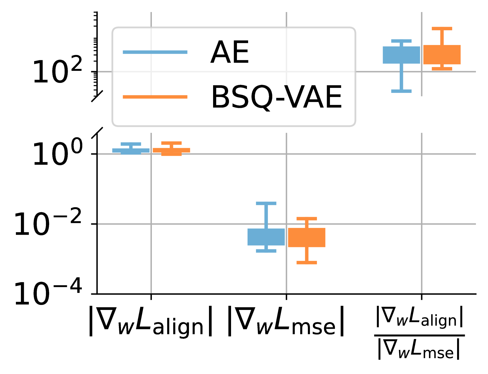
🔼 This figure compares the gradient magnitude for the alignment and reconstruction objectives during the training of QLIP. It visualizes the difference in the convergence rates between these objectives, highlighting the challenge of balancing them effectively. The gradient magnitudes are shown for a linear layer in the visual encoder’s last Multilayer Perceptron (MLP), demonstrating the disparity in the training dynamics between the two objectives.
read the caption
Figure 5: Comparison of gradient magnitude. Here, 𝒘𝒘{\bm{w}}bold_italic_w refers to the linear layer in the visual encoder’s last MLP.

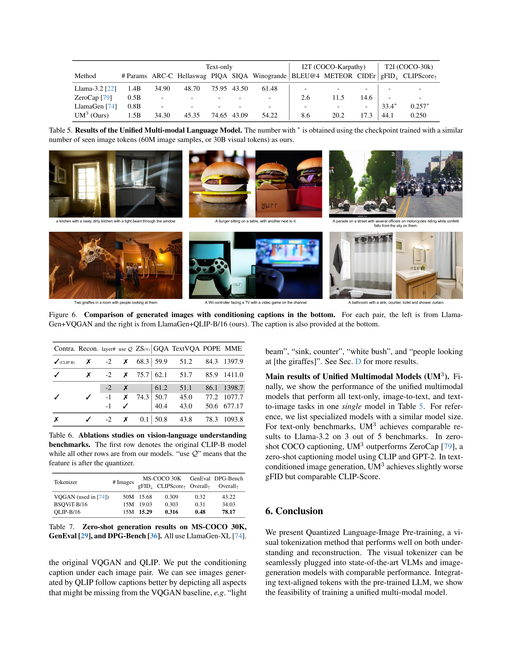
🔼 Figure 6 presents a comparison of images generated using two different visual tokenizers in conjunction with the LlamaGen text-to-image generation model. Each row shows an image pair; the left image is generated using LlamaGen with a VQGAN visual tokenizer, while the right image uses LlamaGen with the QLIP-B/16 tokenizer (the authors’ model). The captions underneath each pair describe the image content.
read the caption
Figure 6: Comparison of generated images with conditioning captions in the bottom. For each pair, the left is from LlamaGen+VQGAN and the right is from LlamaGen+QLIP-B/16 (ours). The caption is also provided at the bottom.
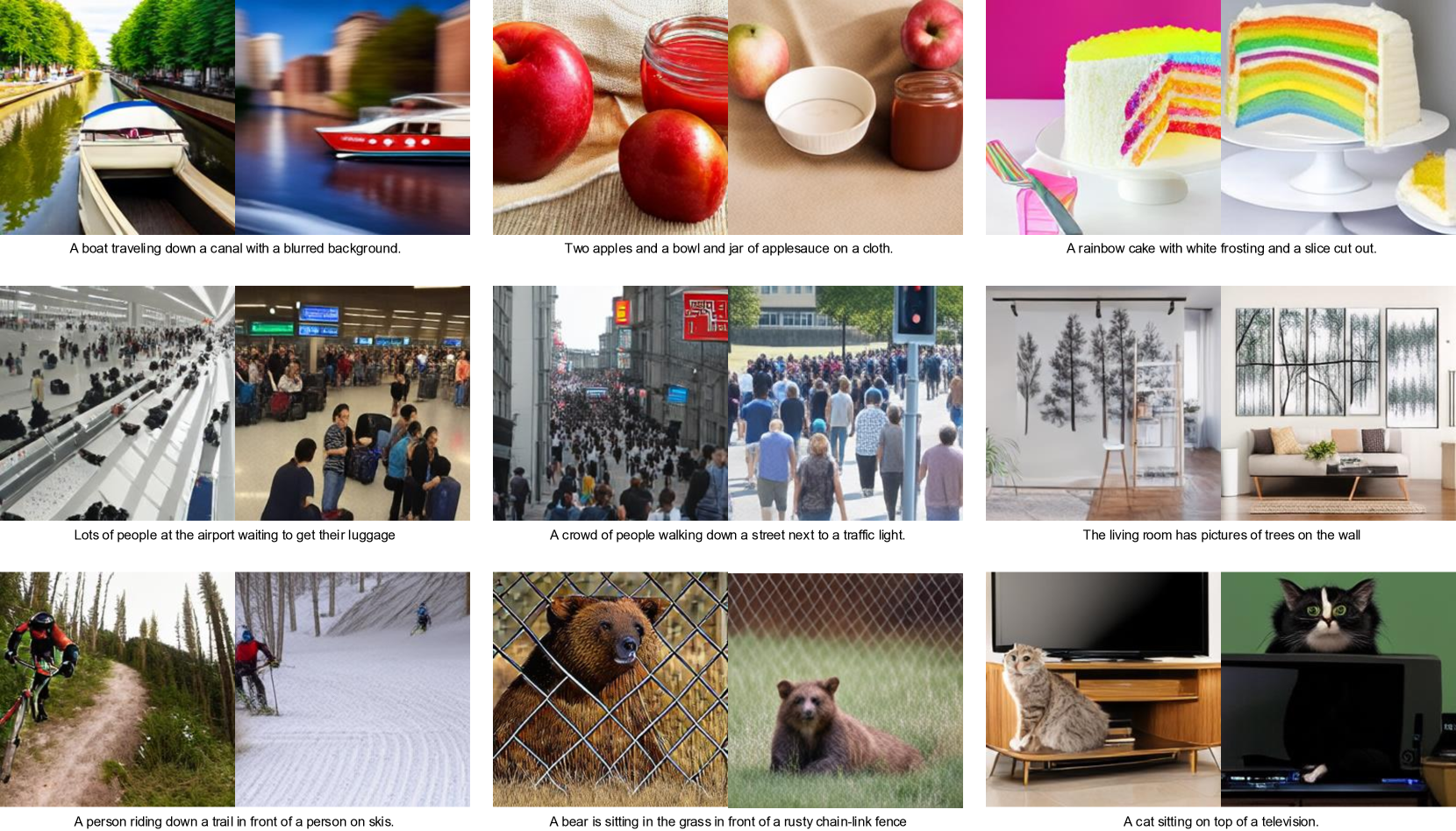
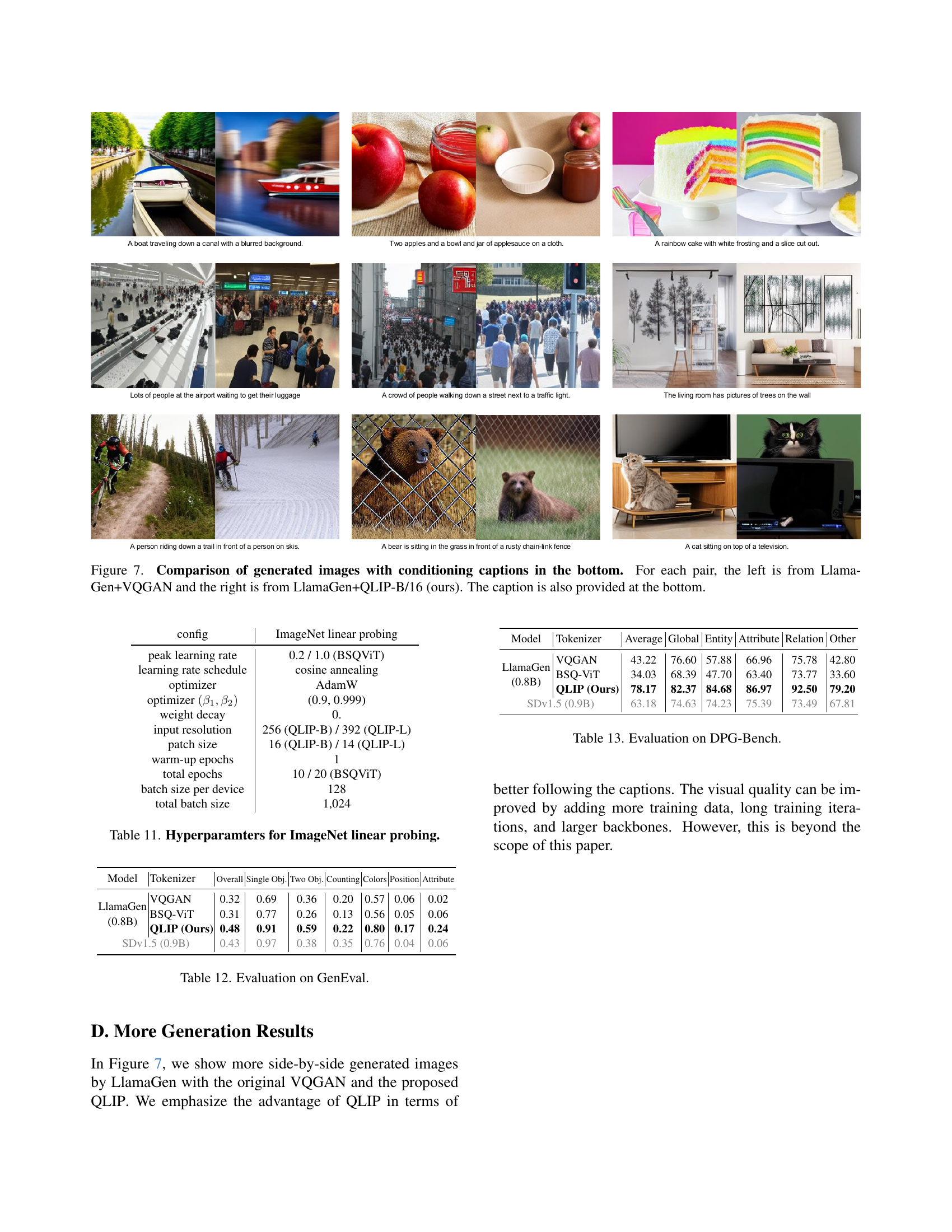
🔼 Figure 7 presents a comparison of images generated using two different visual tokenizers within the LlamaGen framework. Each row shows an image-caption pair. The left image in each pair was generated using LlamaGen with VQGAN as the visual tokenizer, while the right image was generated using LlamaGen with the QLIP-B/16 tokenizer (the authors’ proposed method). The captions accompanying each image are displayed below the image pair for context and comparison.
read the caption
Figure 7: Comparison of generated images with conditioning captions in the bottom. For each pair, the left is from LlamaGen+VQGAN and the right is from LlamaGen+QLIP-B/16 (ours). The caption is also provided at the bottom.
More on tables
| 0-shot | Comp. | Reconstruction | ||||||
| Seen Data | Acc.↑ | # bits | Ratio | rFID↓ | PSNR↑ | SSIM↑ | ||
| (Base backbone) | ||||||||
| CLIP [59] | WIT-400M | 68.3 | / | / | / | / | / | |
| EVA-CLIP [75] | Merged-2B | 74.7 | / | / | / | / | / | |
| SigLIP-B [96] | WL-10B | 76.7 | / | / | / | / | / | |
| VQGAN [24] | IN-1k | / | 14 | 438.8 | 4.98 | - | - | |
| MaskGIT [8] | IN-1k | / | 10 | 614.4 | 1.98 | 18.63 | 0.4619 | |
| MoVQGAN [100] | IN-1k | / | &40 | 153.6 | 1.12 | 22.42 | 0.6731 | |
| RQ-VAE/f32 [44] | IN-1k | / | &112 | 219.4 | 2.69 | - | - | |
| OpenCLIP-B [13] | DC-1B | 73.5 | / | - | / | / | / | |
| BSQViT [98]† | DC-1B | / | 28 | 219.4 | 3.81 | 24.12 | 0.6638 | |
| QLIP-B (ours) | DC-1B | 74.3 | 28 | 219.4 | 3.21 | 23.16 | 0.6286 | |
| (Base backbone, Smaller patch) | ||||||||
| SigLIP-B [96] | WL-10B | 79.2 | / | / | / | / | / | |
| DALL-E dVAE [62] | CC3M+YF | / | 13 | 118.2 | 32.63 | 27.31 | 0.7943 | |
| ViT-VQGAN [91] | IN-1k | / | 13 | 118.2 | 1.55 | - | - | |
| SD-VAE 1.x [63] | OI-2M | / | 14 | 109.7 | 1.40 | 23.65 | 0.6354 | |
| SD-VAE 2.x [58] | OI-2M+LAae | / | #64 | 24 | 0.70 | 26.90 | 0.7592 | |
| SDXL-VAE [58] | OI-2M+LAae++ | / | #64 | 24 | 0.67 | 27.37 | 0.7814 | |
| SBER-MoVQGAN [66] | LAHR-166M | / | 14 | 109.7 | 0.96 | 26.45 | 0.7250 | |
| BSQViT [98] | IN-1k | / | 18 | 85.3 | 0.99 | 27.78 | 0.8171 | |
| EVA-CLIP [75]† | DC-1B | 77.2 | / | / | / | / | / | |
| QLIP-B (ours) | DC-1B | 75.6 | 28 | 54.8 | 0.70 | 26.79 | 0.7905 | |
| (Large backbone) | ||||||||
| CLIP/f14 [59] | WIT-400M | 75.5 | / | / | / | / | / | |
| SigLIP-L [96] | WL-10B | 80.5 | / | / | / | / | / | |
| OpenCLIP-L [13] | DC-1B | 79.2 | / | / | / | / | / | |
| EVA-CLIP-L [75] | Merged-2B | 79.8 | / | / | / | / | / | |
| Open-MAGVIT2 [93, 54] | IN-1k | / | 18 | 85.3 | 1.17 | 21.90 | - | |
| VILA-U [89] | WL-10B+CY-1B | 73.3 | &56 | 27.4 | 1.80 | - | - | |
| (Large backbone, high resolution) | ||||||||
| CLIP/f14 [59] | WIT-400M | 76.6 | / | / | / | / | / | |
| SigLIP-L [96] | WL-10B | 82.1 | / | / | / | / | / | |
| EVA-CLIP-L [75] | Merged-2B | 80.4 | / | / | / | / | / | |
| VILA-U [89] (SO400M) | WL-10B+CY-1B | 78.0 | &224 | 21 | 1.25 | - | - | |
| QLIP-L (ours) | DC-1B | 79.1 | 28 | 168 | 1.46 | 25.36 | 0.6903 | |
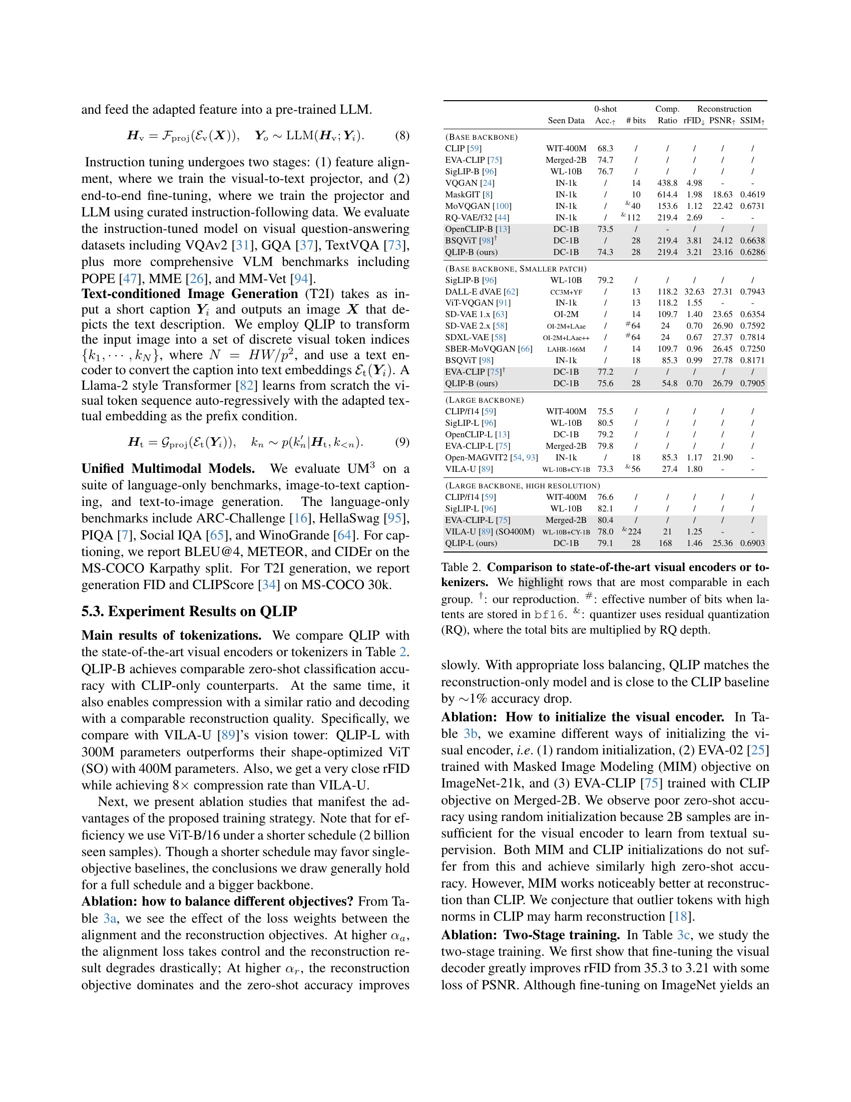
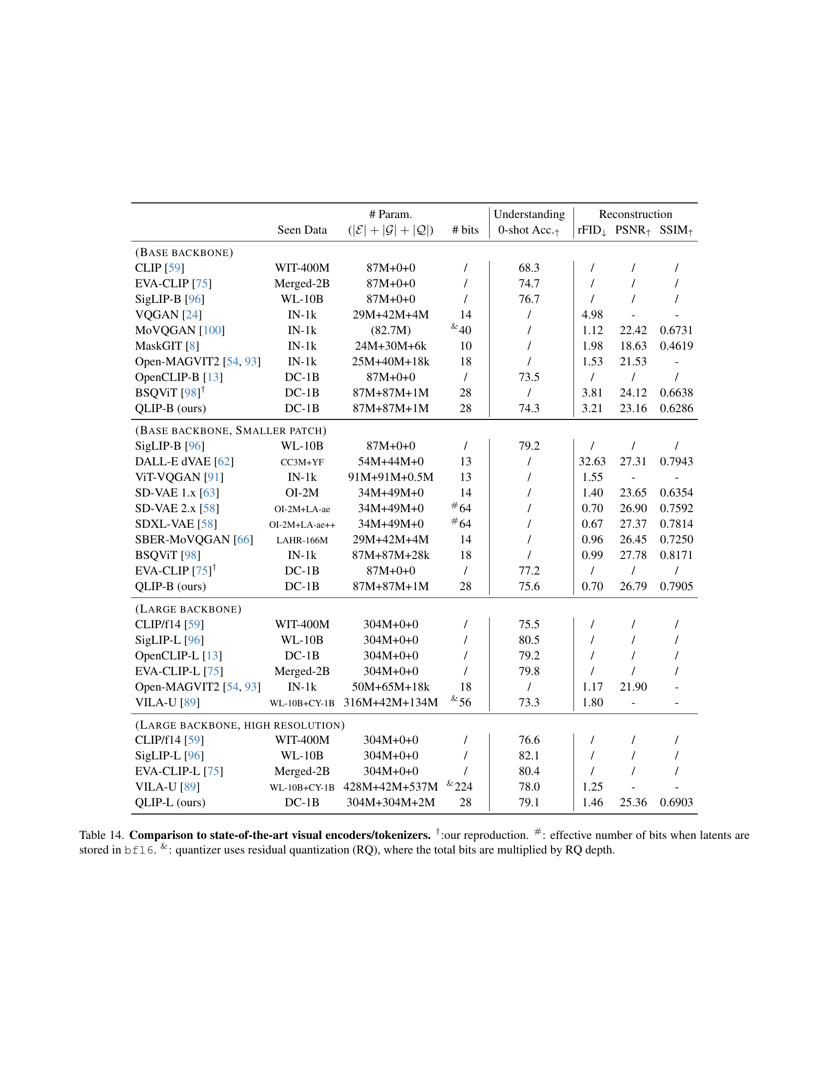
🔼 This table compares QLIP against state-of-the-art visual encoders and tokenizers, focusing on both image understanding (zero-shot accuracy) and reconstruction quality (FID, PSNR, SSIM). It presents results for different model sizes (base, smaller patch, large) and resolutions, highlighting the performance trade-offs between compression and quality. Special notations explain reproduction details and quantizer characteristics.
read the caption
Table 2: Comparison to state-of-the-art visual encoders or tokenizers. We highlight rows that are most comparable in each group. †: our reproduction. #: effective number of bits when latents are stored in bf16. &: quantizer uses residual quantization (RQ), where the total bits are multiplied by RQ depth.
| ZS(%) | RC(rFID)↓ | RC(PSNR) | |
|---|---|---|---|
| 75.7 | 367.8 | 11.7 | |
| 75.1 | 162.6 | 17.8 | |
| 74.7 | 41.7 | 22.5 | |
| 74.3 | 35.3 | 24.5 | |
| 35.4 | 35.6 | 24.5 | |
| 0.1 | 35.7 | 24.5 |
🔼 This table presents ablation study results on the training of QLIP by varying the balance between reconstruction and alignment objectives. It shows how different weightings (αr: αa) for the reconstruction loss (Lmse) and alignment loss (Lalign) impact the zero-shot classification accuracy (ZS) and reconstruction quality measured by rFID and PSNR. Different ratios of αr: αa demonstrate the effect of emphasizing either reconstruction or alignment during training.
read the caption
(a) Balancing Loss.
🔼 This table presents the ablation study on different initialization methods for the visual encoder in the QLIP model. It compares the zero-shot classification accuracy (ZS) and reconstruction performance measured by FID (Frechet Inception Distance), PSNR (Peak Signal-to-Noise Ratio), and SSIM (Structural Similarity Index) across three different initialization strategies: None, Masked Image Modeling (MIM), and CLIP. The results demonstrate the impact of various initialization techniques on the model’s performance in both visual understanding and reconstruction tasks.
read the caption
(b) Initialization.
| ZS(%) | RC(rFID) | RC(PSNR) | ||
|---|---|---|---|---|
| (1) , , , | 35.3 | 24.49 | ||
| Recipe 1 | (2) Finetune | 74.3 | 3.21 | 23.16 |
| (2)∗ (on IN-1k) | 2.90 | 23.33 | ||
| Recipe 2 | (1) , , | 75.0 | 17.2 | 26.72 |
| (2) Train | 13.7 | 23.34 | ||
| + Finetune |
🔼 This table presents ablation studies on training QLIP, focusing on different training recipes. It compares the zero-shot classification accuracy (ZS) and reconstruction quality (measured by FID and PSNR) under various conditions, including different combinations of loss functions (alignment, MSE, etc.), visual encoder initialization methods (random, MIM, CLIP), and whether or not a two-stage training process is used. The results show the impact of each of these factors on the final performance, providing insights into the best training strategy for QLIP.
read the caption
(c) Training Recipe.
| Method | Vision Encoder | Res | LLM | VQAv2 | GQA | TextVQA | POPE | MME | MM-Vet | |
|---|---|---|---|---|---|---|---|---|---|---|
| SEED-X [28] | ViT-bigG-14 | 448 | LLaMA-2-13B | - | 47.9 | - | 84.2 | 1435.7 | - | |
| LaVIT [39] | ViT-G | 224 | LLaMA-2-7B | 68.2 | 48.0 | - | - | - | - | |
| EVE [21] | - | 1344 | Vicuna-1.5-7B | 78.6∗ | 62.6∗ | 56.8 | 85.0 | 1305.7 | 25.7 | |
| Fuyu | - | 1080 | Persimmon-8B | 74.2 | - | - | 74.1 | 728.6 | 21.4 | |
| VILA-U [89] | SigLIP-SO400M | 384 | LLaMA-2-7B | 79.4∗ | 60.8∗ | 60.8 | 85.8 | 1401.8 | 33.5 | |
| Chameleon [77] | VQ-VAE | 512 | LLaMA-2-34B+ | 69.6 | - | - | - | - | - | |
| Show-o [90] | MAGVIT-v2 | 256 | Phi-1.5-1.3B | 59.3∗ | 48.7∗ | - | 73.8 | 948.4 | - | |
| Emu3 [85] | MoVQGAN | 512 | LLaMA-2-8B+ | 75.1∗ | 60.3∗ | 64.7 | 85.2 | - | 37.2 | |
| LLaVA-1.5 [51] | CLIP-Large (orig.) | 336 | Vicuna-1.5-7B | 78.5∗ | 62.0∗ | 58.2 | 85.9 | 1510.7 | 30.5 | |
| CLIP-Large (repro.) | 392 | 79.1∗(+0.0) | 62.3∗(+0.0) | 55.4(+0.0) | 87.5(+0.0) | 1484.9(+0.0) | 33.3(+0.0) | |||
| QLIP-Large (ours) | 392 | 78.3∗(-0.8) | 61.8∗(-0.5) | 55.2(-0.2) | 86.1(-1.4) | 1498.3(+13.4) | 33.3(+0.0) |
🔼 This table presents ablation studies performed on the Quantized Language-Image Pretraining (QLIP) model. It examines the effects of various training strategies and hyperparameters on the model’s performance, specifically focusing on zero-shot classification (ZS) accuracy and reconstruction quality (RC), measured by reconstruction FID (Fréchet Inception Distance) and PSNR (Peak Signal-to-Noise Ratio). The results help to understand the contribution of different components and training choices in achieving the final performance of QLIP.
read the caption
Table 3: Ablation studies of training QLIP. ZS: zero-shot classification; RC: reconstruction. We highlight the default setting.
| Text-only | I2T (COCO-Karpathy) | T2I (COCO-30k) | |||||||||
|---|---|---|---|---|---|---|---|---|---|---|---|
| Method | # Params | ARC-C | Hellaswag | PIQA | SIQA | Winogrande | BLEU@4 | METEOR | CIDEr | gFID↓ | CLIPScore↑ |
| Llama-3.2 [22] | 1.4B | 34.90 | 48.70 | 75.95 | 43.50 | 61.48 | - | - | - | - | - |
| ZeroCap [79] | 0.5B | - | - | - | - | - | 2.6 | 11.5 | 14.6 | - | - |
| LlamaGen [74] | 0.8B | - | - | - | - | - | - | - | - | 33.4∗ | 0.257∗ |
| UM3 (Ours) | 1.5B | 34.30 | 45.35 | 74.65 | 43.09 | 54.22 | 8.6 | 20.2 | 17.3 | 44.1 | 0.250 |
🔼 Table 4 presents a comparison of vision-language understanding performance between various models, including QLIP and LLaVA-1.5. It evaluates models across multiple benchmark datasets (VQAv2, GQA, TextVQA, POPE, MME, MM-Vet) commonly used to assess vision-language capabilities. The results highlight QLIP’s performance in relation to established methods and shows that when using a controlled experimental setup with a reproduced CLIP-Large model, QLIP’s encoder achieves comparable performance to LLaVA-1.5.
read the caption
Table 4: Comparison to vision-language modeling on vision-language understanding benchmarks. QLIP’s encoder works on par with LLaVA-1.5 with our reproduced CLIP-Large under a controlled experiment.
| Contra. | Recon. | layer# | use | ZS(%) | GQA | TextVQA | POPE | MME |
|---|---|---|---|---|---|---|---|---|
| ✓(CLIP-B) | ✗ | -2 | ✗ | 68.3 | 59.9 | 51.2 | 84.3 | 1397.9 |
| ✓ | ✗ | -2 | ✗ | 75.7 | 62.1 | 51.7 | 85.9 | 1411.0 |
| ✓ | ✓ | -2 | ✗ | 74.3 | 61.2 | 51.1 | 86.1 | 1398.7 |
| -1 | ✗ | 50.7 | 45.0 | 77.2 | 1077.7 | |||
| -1 | ✓ | 40.4 | 43.0 | 50.6 | 677.17 | |||
| ✗ | ✓ | -2 | ✗ | 0.1 | 50.8 | 43.8 | 78.3 | 1093.8 |
🔼 This table presents the performance of the Unified Multimodal Model (UM³) on various benchmarks. It compares the UM³’s results on language-only tasks (ARC-Challenge, HellaSwag, PIQA, SocialIQA, Winogrande), image-to-text captioning (BLEU@4, METEOR, CIDEr), and text-to-image generation (FID, CLIPScore). The asterisk (*) indicates results obtained using a checkpoint trained with a similar number of image tokens (60 million image samples, or 30 billion visual tokens) as the primary UM³ model.
read the caption
Table 5: Results of the Unified Multi-modal Language Model. The number with ∗ is obtained using the checkpoint trained with a similar number of seen image tokens (60M image samples, or 30B visual tokens) as ours.
| Tokenizer | # Images | MS-COCO 30K | GenEval | DPG-Bench | |
|---|---|---|---|---|---|
| gFID↓ | CLIPScore↑ | Overall↑ | Overall↑ | ||
| VQGAN (used in [74]) | 50M | 15.68 | 0.309 | 0.32 | 43.22 |
| BSQViT-B/16 | 15M | 19.03 | 0.303 | 0.31 | 34.03 |
| QLIP-B/16 | 15M | 15.29 | 0.316 | 0.48 | 78.17 |
🔼 This ablation study investigates the impact of various design choices within the QLIP model on vision-language understanding performance. The table compares the original CLIP-B model (row 1) to several variants of the QLIP model (rows 2-7). These variations explore different aspects: the inclusion of the contrastive loss (✓ or ✗), the stage at which the quantizer is used (-1 or -2, indicating the layer before or after the quantizer is used), and whether the quantizer is employed (✓ or ✗). Each row shows the zero-shot accuracy (ZS) and scores on the GQA, TextVQA, POPE, and MM-Vet benchmarks. This analysis helps determine the contribution of different components of the QLIP architecture to its overall effectiveness in vision-language understanding tasks.
read the caption
Table 6: Ablations studies on vision-language understanding benchmarks. The first row denotes the original CLIP-B model while all other rows are from our models. “use 𝒬𝒬{\mathcal{Q}}caligraphic_Q” means that the feature is after the quantizer.
| config | Stage 1 | Stage 2 |
| peak learning rate | 5e-4 | 5e-4 |
| learning rate | 2e-4 | 0 |
| learning rate | 2e-5 | 0 |
| learning rate | 2e-3 | 1e-4 |
| learning rate schedule | cosine annealing | cosine annealing |
| optimizer | LAMB | AdamW |
| optimizer | (0.9, 0.95) | (0.9, 0.95) |
| weight decay | 0.05 | 0.05 |
| gradient clip | 5 | 1 |
| input resolution | 256 | 256 |
| patch size | 8 | 8 |
| warm-up iterations | 2,000 | 2,000 |
| total iterations | 120,000 | 120,000 |
| batch size per device | 512 | 128 |
| total batch size | 65,536 | 16,384 |
| optimizer | - | AdamW |
| learning rate | - | 1e-4 |
| reconstruction loss weight | 1e3 | 1 |
| contrastive loss weight | 1 | 0 |
| quantization loss weight | 1 | 1 |
| perceptual loss weight | 0 | 0.1 |
| GAN loss weight | 0 | 0.1 |
| commitment loss weight | 1.0 | 0 |
🔼 This table presents a comparison of zero-shot image generation performance using different visual tokenizers within the LlamaGen-XL framework. It shows the FID (Fréchet Inception Distance) and CLIPScore metrics for image generation quality on three benchmark datasets: MS-COCO 30K, GenEval, and DPG-Bench. Lower FID indicates better image quality, while higher CLIPScore indicates better alignment between generated images and their captions. The results allow for an evaluation of how different visual tokenization methods impact the overall quality and semantic consistency of the generated images.
read the caption
Table 7: Zero-shot generation results on MS-COCO 30K, GenEval [29], and DPG-Bench [36]. All use LlamaGen-XL [74].
| config | Training UM3 |
|---|---|
| peak learning rate | 1e-4 |
| learning rate schedule | cosine annealing |
| optimizer | AdamW |
| optimizer | (0.9, 0.95) |
| weight decay | 0.1 |
| gradient clip | 1 |
| warm-up iterations | 2,000 |
| total iterations | 600,000 |
| batch size per device | 8 |
| total batch size | 512 |
| sequence length | 4,096 |
| calm-down steps | 10,000 |
| mix ratio () | 60:1:3 |
| mix ratio () | 12:1:3 |
| sampling temperature | 1.0 |
| sampling top- | 0.95 |
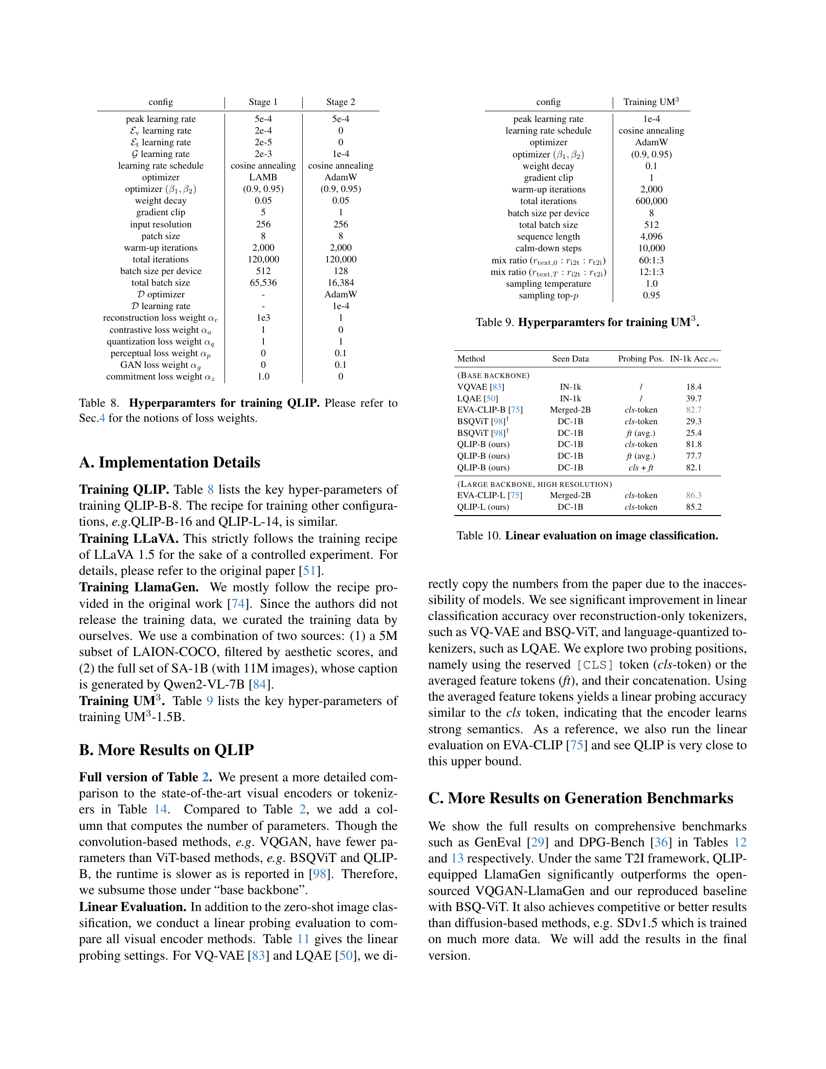
🔼 This table details the hyperparameters used during the training of the Quantized Language-Image Pretraining (QLIP) model. It shows the settings for both Stage 1 and Stage 2 of the training process. Stage 1 focuses on joint optimization of alignment and reconstruction losses, while Stage 2 fine-tunes the model with a focus on reconstruction quality. The table includes parameters such as learning rates for different components of the model (visual encoder, text encoder, decoder, and quantizer), optimization algorithm, weight decay, gradient clipping, batch sizes, and the number of training iterations. Crucially, it also lists the weights assigned to the different loss functions (reconstruction, contrastive, and quantization losses) during each stage. Section 4 of the paper provides further details on these loss functions and their balancing.
read the caption
Table 8: Hyperparamters for training QLIP. Please refer to Sec.4 for the notions of loss weights.
| Method | Seen Data | Probing Pos. | IN-1k Acc.(%) |
| (Base backbone) | |||
| VQVAE [83] | IN-1k | / | 18.4 |
| LQAE [50] | IN-1k | / | 39.7 |
| EVA-CLIP-B [75] | Merged-2B | cls-token | 82.7 |
| BSQViT [98]† | DC-1B | cls-token | 29.3 |
| BSQViT [98]† | DC-1B | ft (avg.) | 25.4 |
| QLIP-B (ours) | DC-1B | cls-token | 81.8 |
| QLIP-B (ours) | DC-1B | ft (avg.) | 77.7 |
| QLIP-B (ours) | DC-1B | cls + ft | 82.1 |
| (Large backbone, high resolution) | |||
| EVA-CLIP-L [75] | Merged-2B | cls-token | 86.3 |
| QLIP-L (ours) | DC-1B | cls-token | 85.2 |
🔼 This table lists the hyperparameters used for training the Unified Multimodal Model (UM³), a model that unifies understanding and generation across multiple modalities. It details settings for various aspects of the training process, including optimizer choices, learning rates, scheduling strategies, batch sizes, and other relevant parameters. This configuration is crucial for the UM³ model’s ability to handle text-only, image-to-text, and text-to-image tasks.
read the caption
Table 9: Hyperparamters for training UM3.
| config | ImageNet linear probing |
|---|---|
| peak learning rate | 0.2 / 1.0 (BSQViT) |
| learning rate schedule | cosine annealing |
| optimizer | AdamW |
| optimizer | (0.9, 0.999) |
| weight decay | 0. |
| input resolution | 256 (QLIP-B) / 392 (QLIP-L) |
| patch size | 16 (QLIP-B) / 14 (QLIP-L) |
| warm-up epochs | 1 |
| total epochs | 10 / 20 (BSQViT) |
| batch size per device | 128 |
| total batch size | 1,024 |
🔼 This table presents the results of a linear evaluation experiment on image classification. It compares various visual encoder methods, including those based on VQ-VAE, LQAE, EVA-CLIP, BSQViT, and QLIP, to assess their performance on this task. The evaluation uses two probing positions for the features extracted by the visual encoders: either the [CLS] token or the average of all feature tokens. The table also includes a combination of both for comparison. The goal is to evaluate the quality of visual representations learned by different visual encoders and how well these representations generalize to downstream image classification tasks.
read the caption
Table 10: Linear evaluation on image classification.
| Model | Tokenizer | Overall | Single Obj. | Two Obj. | Counting | Colors | Position | Attribute |
|---|---|---|---|---|---|---|---|---|
| LlamaGen | VQGAN | 0.32 | 0.69 | 0.36 | 0.20 | 0.57 | 0.06 | 0.02 |
| (0.8B) | BSQ-ViT | 0.31 | 0.77 | 0.26 | 0.13 | 0.56 | 0.05 | 0.06 |
| QLIP (Ours) | 0.48 | 0.91 | 0.59 | 0.22 | 0.80 | 0.17 | 0.24 | |
| SDv1.5 (0.9B) | 0.43 | 0.97 | 0.38 | 0.35 | 0.76 | 0.04 | 0.06 | |
🔼 This table lists the hyperparameters used for the ImageNet linear probing experiments. It details settings for the learning rate, optimizer, weight decay, input resolution, patch size, training epochs, batch size, and other relevant parameters used in evaluating the performance of visual encoders through linear probing on the ImageNet dataset. This is important for understanding how different configurations impact the model’s performance on this specific task.
read the caption
Table 11: Hyperparamters for ImageNet linear probing.
| Model | Tokenizer | Average | Global | Entity | Attribute | Relation | Other |
|---|---|---|---|---|---|---|---|
| LlamaGen | VQGAN | 43.22 | 76.60 | 57.88 | 66.96 | 75.78 | 42.80 |
| (0.8B) | BSQ-ViT | 34.03 | 68.39 | 47.70 | 63.40 | 73.77 | 33.60 |
| QLIP (Ours) | 78.17 | 82.37 | 84.68 | 86.97 | 92.50 | 79.20 | |
| SDv1.5 (0.9B) | 63.18 | 74.63 | 74.23 | 75.39 | 73.49 | 67.81 | |
🔼 This table presents a quantitative comparison of different visual tokenizers on the GenEval benchmark. GenEval is a comprehensive evaluation benchmark designed to assess various aspects of image generation models beyond standard metrics like FID. It includes sub-scores for evaluating the generation of different types of images, including those with single objects, multiple objects, specific counts, colors, or other attributes. The table shows each model’s overall performance and its performance broken down by these sub-categories to offer a more nuanced understanding of their strengths and weaknesses.
read the caption
Table 12: Evaluation on GenEval.
| # Param. | Understanding | Reconstruction | |||||||
| Seen Data | () | # bits | 0-shot Acc.↑ | rFID↓ | PSNR↑ | SSIM↑ | |||
| (Base backbone) | |||||||||
| CLIP [59] | WIT-400M | 87M+0+0 | / | 68.3 | / | / | / | ||
| EVA-CLIP [75] | Merged-2B | 87M+0+0 | / | 74.7 | / | / | / | ||
| SigLIP-B [96] | WL-10B | 87M+0+0 | / | 76.7 | / | / | / | ||
| VQGAN [24] | IN-1k | 29M+42M+4M | 14 | / | 4.98 | - | - | ||
| MoVQGAN [100] | IN-1k | (82.7M) | &40 | / | 1.12 | 22.42 | 0.6731 | ||
| MaskGIT [8] | IN-1k | 24M+30M+6k | 10 | / | 1.98 | 18.63 | 0.4619 | ||
| Open-MAGVIT2 [93, 54] | IN-1k | 25M+40M+18k | 18 | / | 1.53 | 21.53 | - | ||
| OpenCLIP-B [13] | DC-1B | 87M+0+0 | / | 73.5 | / | / | / | ||
| BSQViT [98]† | DC-1B | 87M+87M+1M | 28 | / | 3.81 | 24.12 | 0.6638 | ||
| QLIP-B (ours) | DC-1B | 87M+87M+1M | 28 | 74.3 | 3.21 | 23.16 | 0.6286 | ||
| (Base backbone, Smaller patch) | |||||||||
| SigLIP-B [96] | WL-10B | 87M+0+0 | / | 79.2 | / | / | / | ||
| DALL-E dVAE [62] | CC3M+YF | 54M+44M+0 | 13 | / | 32.63 | 27.31 | 0.7943 | ||
| ViT-VQGAN [91] | IN-1k | 91M+91M+0.5M | 13 | / | 1.55 | - | - | ||
| SD-VAE 1.x [63] | OI-2M | 34M+49M+0 | 14 | / | 1.40 | 23.65 | 0.6354 | ||
| SD-VAE 2.x [58] | OI-2M+LA-ae | 34M+49M+0 | #64 | / | 0.70 | 26.90 | 0.7592 | ||
| SDXL-VAE [58] | OI-2M+LA-ae++ | 34M+49M+0 | #64 | / | 0.67 | 27.37 | 0.7814 | ||
| SBER-MoVQGAN [66] | LAHR-166M | 29M+42M+4M | 14 | / | 0.96 | 26.45 | 0.7250 | ||
| BSQViT [98] | IN-1k | 87M+87M+28k | 18 | / | 0.99 | 27.78 | 0.8171 | ||
| EVA-CLIP [75]† | DC-1B | 87M+0+0 | / | 77.2 | / | / | / | ||
| QLIP-B (ours) | DC-1B | 87M+87M+1M | 28 | 75.6 | 0.70 | 26.79 | 0.7905 | ||
| (Large backbone) | |||||||||
| CLIP/f14 [59] | WIT-400M | 304M+0+0 | / | 75.5 | / | / | / | ||
| SigLIP-L [96] | WL-10B | 304M+0+0 | / | 80.5 | / | / | / | ||
| OpenCLIP-L [13] | DC-1B | 304M+0+0 | / | 79.2 | / | / | / | ||
| EVA-CLIP-L [75] | Merged-2B | 304M+0+0 | / | 79.8 | / | / | / | ||
| Open-MAGVIT2 [93, 54] | IN-1k | 50M+65M+18k | 18 | / | 1.17 | 21.90 | - | ||
| VILA-U [89] | WL-10B+CY-1B | 316M+42M+134M | &56 | 73.3 | 1.80 | - | - | ||
| (Large backbone, high resolution) | |||||||||
| CLIP/f14 [59] | WIT-400M | 304M+0+0 | / | 76.6 | / | / | / | ||
| SigLIP-L [96] | WL-10B | 304M+0+0 | / | 82.1 | / | / | / | ||
| EVA-CLIP-L [75] | Merged-2B | 304M+0+0 | / | 80.4 | / | / | / | ||
| VILA-U [89] | WL-10B+CY-1B | 428M+42M+537M | &224 | 78.0 | 1.25 | - | - | ||
| QLIP-L (ours) | DC-1B | 304M+304M+2M | 28 | 79.1 | 1.46 | 25.36 | 0.6903 | ||
🔼 This table presents a quantitative evaluation of different visual tokenizers on the DPG-Bench benchmark, specifically focusing on text-to-image generation. The benchmark assesses performance across various aspects of image generation quality, including average global scores, entity, attribute, relation, and other aspects. It allows for a comparison of different approaches in terms of how well-generated images align with given captions, and how effectively they represent details within the image.
read the caption
Table 13: Evaluation on DPG-Bench.
Full paper#