TL;DR#
Current context-augmented generation (CAG) methods face challenges in handling long sequences due to the computational burden of re-encoding all contexts for every query. This issue restricts the use of large contexts, limiting performance. Many existing attempts rely on computationally expensive and less effective fine-tuning.
The paper introduces Adaptive Parallel Encoding (APE), a novel method that pre-computes and caches context embeddings, enabling efficient retrieval and integration. By incorporating shared prefixes, adjusting temperature, and applying a scaling factor, APE aligns parallel encoding’s distribution with sequential encoding, achieving a substantial 4.5x speedup for a 128K-length context while maintaining high accuracy. APE outperforms previous methods in both RAG and ICL tasks.
Key Takeaways#
Why does it matter?#
This paper is crucial for researchers working on context-augmented generation because it introduces a novel technique that significantly improves the efficiency and scalability of existing methods. The proposed approach, Adaptive Parallel Encoding (APE), addresses a major bottleneck in current CAG systems, opening new avenues for research in handling long-context inputs and many-shot learning scenarios. The speedup achieved makes long-context applications more practical, and the findings are relevant to a wide range of fields using LLMs.
Visual Insights#

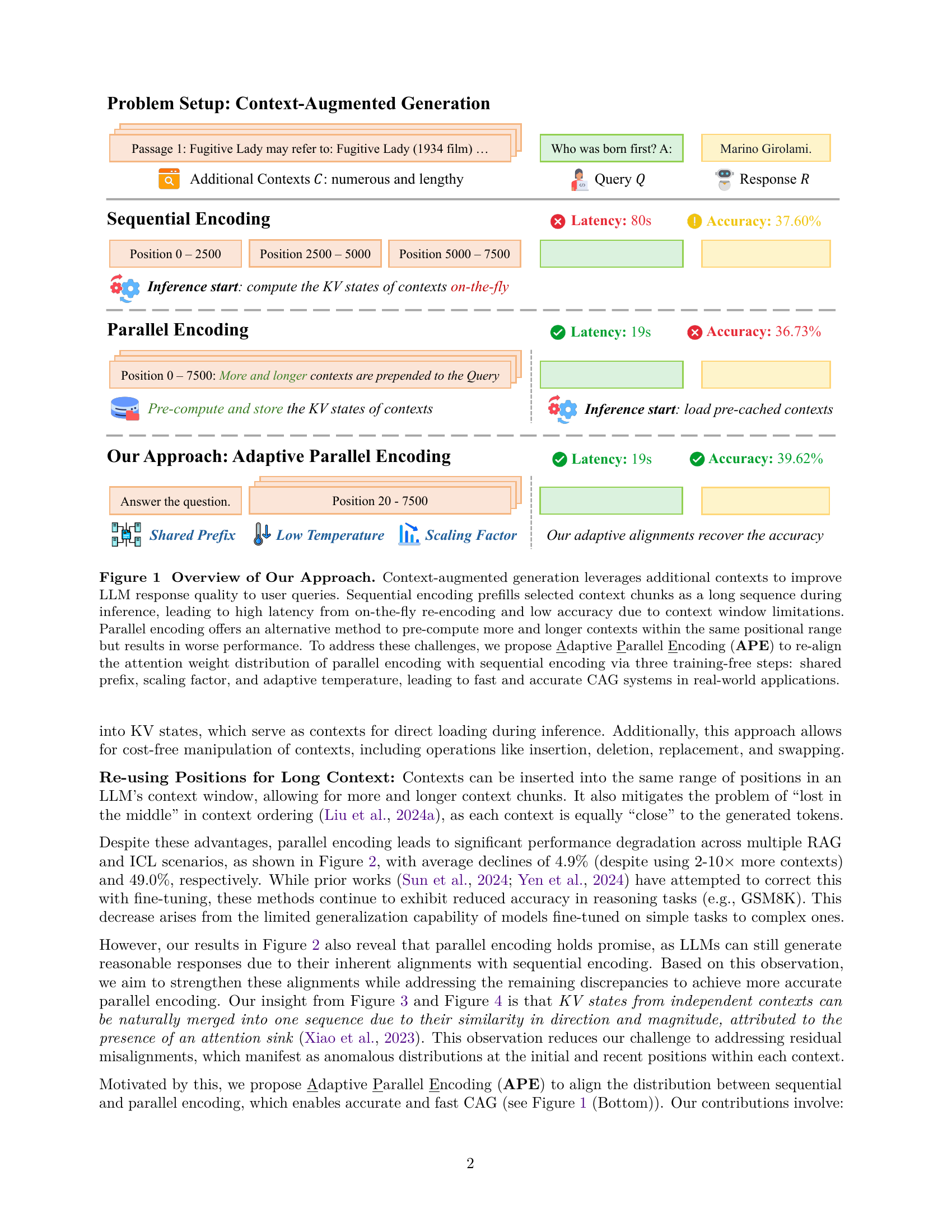
🔼 Figure 1 illustrates the core concept of Adaptive Parallel Encoding (APE) and its advantages over traditional methods in context-augmented generation (CAG). It highlights three key approaches: sequential encoding (encoding all contexts as a single sequence, leading to high latency and limited accuracy due to context window limitations), parallel encoding (independently pre-computing contexts, leading to faster inference but lower accuracy due to misalignments in attention), and APE (the proposed method that uses a shared prefix, attention temperature, and scaling factor to align parallel encoding with sequential encoding, achieving both speed and accuracy improvements). The figure visually represents the workflow of each method, contrasting their performance in terms of inference speed and accuracy.
read the caption
Figure 1: Overview of Our Approach. Context-augmented generation leverages additional contexts to improve LLM response quality to user queries. Sequential encoding prefills selected context chunks as a long sequence during inference, leading to high latency from on-the-fly re-encoding and low accuracy due to context window limitations. Parallel encoding offers an alternative method to pre-compute more and longer contexts within the same positional range but results in worse performance. To address these challenges, we propose Adaptive Parallel Encoding (APE) to re-align the attention weight distribution of parallel encoding with sequential encoding via three training-free steps: shared prefix, scaling factor, and adaptive temperature, leading to fast and accurate CAG systems in real-world applications.
| Method | INSCIT | Doc2Dial | TopicCQA | Qrecc | QuAC | Average |
|---|---|---|---|---|---|---|
| Contriever, Sequential | 19.97 | 23.85 | 30.49 | 46.75 | 26.57 | 29.53 |
| Contriever, APE | 19.88 | 23.28 | 28.84 | 46.28 | 26.80 | 29.02 |
| -0.09 | -0.57 | -1.65 | -0.47 | +0.23 | -0.51 | |
| GTE-base, Sequential | 21.58 | 32.35 | 33.41 | 46.54 | 30.69 | 32.91 |
| GTE-base, APE | 20.85 | 30.99 | 31.92 | 45.83 | 30.35 | 31.99 |
| -0.73 | -1.36 | -1.49 | -0.71 | -0.34 | -0.92 | |
| Dragon-multiturn, Sequential | 25.42 | 36.27 | 36.10 | 49.01 | 35.12 | 36.38 |
| Dragon-multiturn, APE | 23.84 | 34.93 | 33.80 | 48.70 | 34.92 | 35.24 |
| -1.58 | -1.34 | -2.30 | -0.31 | -0.20 | -1.14 | |
| All texts, APE | 27.22 | 36.13 | 35.72 | 49.15 | 35.70 | 36.78 |
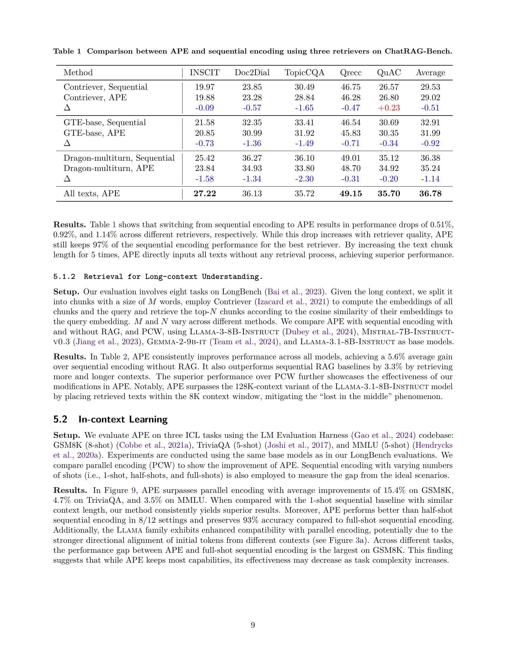
🔼 This table presents a comparison of the performance of Adaptive Parallel Encoding (APE) against sequential encoding methods on the ChatRAG-Bench benchmark. The comparison uses three different retrievers (Contriever, GTE-base, and Dragon-multiturn) to retrieve relevant information for generating answers. For each retriever, the table shows the average F1 scores across various subtasks (INSCIT, Doc2Dial, TopicCQA, Qrecc, QuAC), and the overall average across all tasks. The differences between APE and sequential encoding are highlighted, demonstrating APE’s performance gains or losses for each retriever.
read the caption
Table 1: Comparison between APE and sequential encoding using three retrievers on ChatRAG-Bench.
In-depth insights#
Adaptive Parallel Encoding#
The concept of “Adaptive Parallel Encoding” presented in the research paper addresses the computational bottleneck in context-augmented generation (CAG) methods like RAG and ICL. Traditional approaches suffer from high latency due to the sequential encoding of multiple contexts for each query. Adaptive Parallel Encoding (APE) tackles this by independently pre-computing and caching the key-value (KV) states of each context. This allows for the direct loading of cached states during inference, significantly speeding up the process. However, a naive parallel encoding approach leads to accuracy drops. Therefore, APE introduces three key innovations: a shared prefix to handle misalignments in the attention distribution, an adaptive temperature to sharpen attention, and a scaling factor to correct for magnitude discrepancies. The results demonstrate that APE successfully preserves a high percentage of sequential encoding’s performance while significantly outperforming traditional parallel encoding across multiple tasks and demonstrating scalability to handle many-shot CAG scenarios. The overall efficiency improvements, including a substantial reduction in context prefilling time, make APE a promising technique for improving the practical applicability of CAG in real-world deployments.
Long context efficiency#
Long context efficiency in large language models (LLMs) is a critical area of research, focusing on enabling LLMs to process and generate coherent outputs from significantly larger input contexts than previously possible. The core challenge lies in the computational cost of encoding and attending to these extended contexts. Approaches like retrieval augmented generation (RAG) attempt to mitigate this by retrieving only the most relevant information, but this introduces complexities in retrieval and selection. Adaptive Parallel Encoding (APE) in this paper addresses the efficiency bottleneck of encoding long contexts by pre-computing and caching each context’s key-value (KV) states. This reduces the computational burden at inference time, enabling much faster response generation. However, simply parallelizing the encoding process can lead to performance degradation; therefore, APE introduces techniques like shared prefix, attention temperature, and scaling factor to mitigate this, significantly improving accuracy while maintaining speed. The overall goal is to unlock the full potential of LLMs by allowing them to leverage the wealth of information available in long contexts while maintaining practical efficiency. This involves balancing the increased model capacity needed to process long contexts with optimization strategies that prevent latency from becoming a major limitation. APE’s effectiveness in achieving this balance is highlighted by significant speed improvements and a minimal accuracy trade-off. Future research may focus on exploring further optimization techniques to minimize memory usage while maximizing long-context performance.
Attention alignment#
Attention alignment in the context of large language models (LLMs) and context-augmented generation (CAG) is crucial for performance. Misalignments between parallel and sequential encoding of contexts lead to accuracy drops, as observed in the paper. The core of the problem lies in the differing attention weight distributions produced by these two methods. Techniques like shared prefixes, adjusted attention temperatures, and scaling factors are proposed to mitigate these differences. By subtly altering the attention distribution during parallel encoding, these methods aim to bring it closer to the distribution obtained with sequential encoding. The success of these methods demonstrates the importance of carefully managing attention mechanisms to leverage the efficiency of parallel processing while preserving the accuracy of sequential models. Future work could explore more sophisticated alignment techniques that go beyond these simple heuristics, perhaps leveraging learned models or more nuanced analysis of attention patterns to optimize alignment dynamically based on context characteristics.
Many-shot scalability#
The many-shot scalability of APE is a crucial aspect of its effectiveness for real-world applications. The paper demonstrates that APE maintains high accuracy even when handling hundreds of contexts, significantly outperforming traditional parallel encoding methods and approaching the accuracy of sequential encoding. This is achieved without the need for further training, thus highlighting APE’s efficiency and practicality. The ability to effectively manage many-shot scenarios is a major advantage over existing methods, particularly for tasks involving extensive contextual information. This scalability stems from APE’s ability to pre-compute and cache KV states effectively, allowing for the efficient loading of relevant information at inference time. The efficient pre-computation drastically reduces the bottleneck in the context prefilling process, which is often a major constraint in traditional CAG methods. The results show substantial speed improvements and maintains accuracy, highlighting the effectiveness of APE’s approach in handling complex, long-context tasks. While the paper focuses on RAG and ICL tasks, the findings suggest that APE’s many-shot scalability could be generalized to other applications requiring the efficient integration of diverse and extensive contextual information.
APE limitations#
The heading ‘APE limitations’ would ideally discuss the shortcomings of the Adaptive Parallel Encoding (APE) method presented in the research paper. A thoughtful analysis would likely highlight that while APE offers significant speed improvements for context-augmented generation, it’s not without its drawbacks. One key limitation is APE’s sensitivity to hyperparameter tuning. The optimal settings for attention temperature and scaling factor might vary considerably across different tasks and datasets, necessitating careful experimentation and potentially limiting the method’s ease of use and generalizability. Furthermore, the effectiveness of APE’s alignment strategies could be affected by the variability in context length, quantity, and content found in real-world applications. In scenarios with highly diverse contexts, maintaining an accurate and efficient alignment between parallel and sequential encoding could pose a challenge. Additionally, the reliance on pre-computed KV states, although accelerating inference, introduces memory and storage requirements, which might become substantial with a large number of contexts. Finally, a thorough limitations section should acknowledge the relatively simpler nature of the experiments conducted, suggesting the need for further evaluation on more complex tasks and larger-scale datasets to fully assess the robustness and practical applicability of the APE technique.
More visual insights#
More on figures

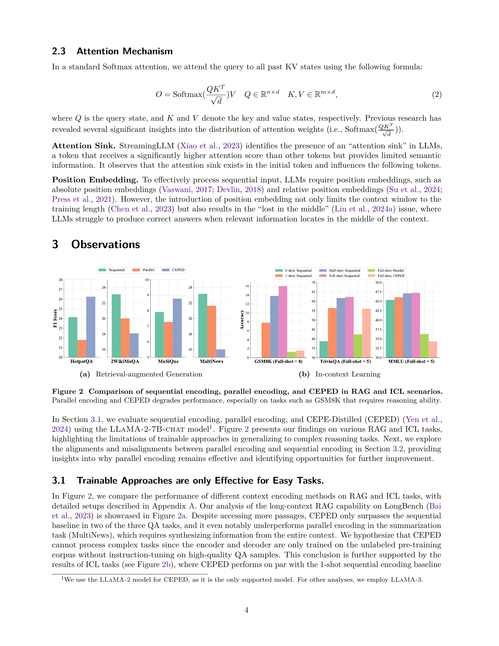
🔼 This figure shows the performance comparison of three different context encoding methods (sequential encoding, parallel encoding, and CEPED) on several retrieval-augmented generation (RAG) tasks. The x-axis represents different RAG tasks, and the y-axis represents the F1 score. Sequential encoding shows the best performance, while parallel encoding and CEPED both underperform significantly, particularly on tasks that require complex reasoning abilities.
read the caption
(a) Retrieval-augmented Generation

🔼 This figure displays the results of in-context learning experiments. It compares the performance of sequential encoding, parallel encoding, and a fine-tuned model (CEPED) across various tasks. The performance is measured using F1 score and accuracy, enabling a comparison of the different methods’ abilities to generalize to various ICL tasks of differing complexity.
read the caption
(b) In-context Learning

🔼 This figure compares the performance of three different context encoding methods: sequential encoding, parallel encoding, and CEPE-Distilled (CEPED), across various retrieval-augmented generation (RAG) and in-context learning (ICL) tasks. The results show that while parallel encoding offers faster inference times by encoding contexts separately, it significantly reduces accuracy compared to sequential encoding. CEPED, a trainable approach, also underperforms sequential encoding, particularly on tasks requiring complex reasoning, such as GSM8K. The figure highlights the limitations of parallel encoding and trainable methods in achieving both efficiency and accuracy in context-augmented generation.
read the caption
Figure 2: Comparison of sequential encoding, parallel encoding, and CEPED in RAG and ICL scenarios. Parallel encoding and CEPED degrades performance, especially on tasks such as GSM8K that requires reasoning ability.

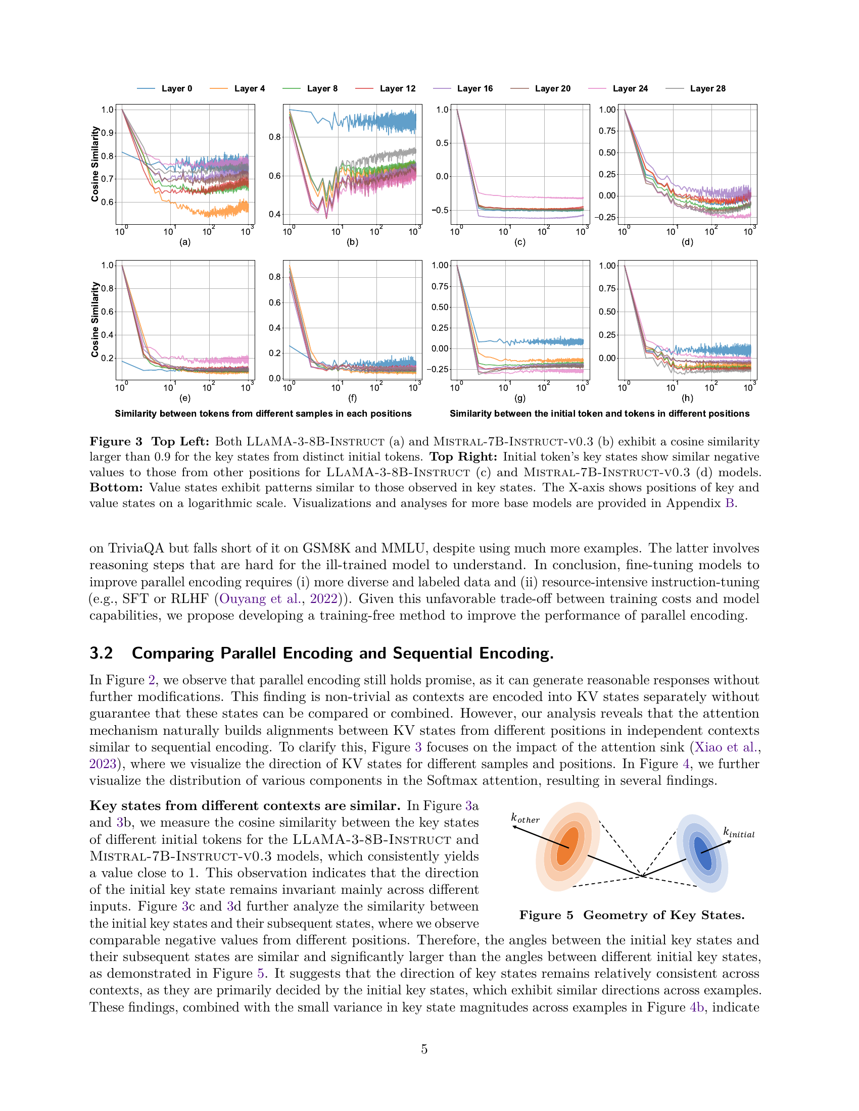
🔼 Figure 3 analyzes the distribution of key and value states in LLMs, specifically focusing on the impact of the attention sink. The top row shows that the initial key states from different samples have a high cosine similarity (above 0.9) for both LLaMA-3-8B-Instruct and Mistral-7B-Instruct-v0.3. The top right demonstrates that initial key states share similar negative values with those from other positions. The bottom row shows that value states exhibit patterns consistent with the observations made for key states. This analysis uses a logarithmic scale for the x-axis (position of key/value states). Further analysis for additional LLMs is provided in Appendix B.
read the caption
Figure 3: Top Left: Both LLaMA-3-8B-Instruct (a) and Mistral-7B-Instruct-v0.3 (b) exhibit a cosine similarity larger than 0.9 for the key states from distinct initial tokens. Top Right: Initial token’s key states show similar negative values to those from other positions for LLaMA-3-8B-Instruct (c) and Mistral-7B-Instruct-v0.3 (d) models. Bottom: Value states exhibit patterns similar to those observed in key states. The X-axis shows positions of key and value states on a logarithmic scale. Visualizations and analyses for more base models are provided in Appendix 11.

🔼 This figure visualizes the cosine similarity between query and key states across different layers and positions. The x-axis represents the position of key states (log scale), while the y-axis shows the cosine similarity. Different colored lines correspond to different layers in the model. The figure helps to understand how the similarity changes with respect to position. A high similarity indicates strong attention.
read the caption
(a) Query-Key Similarity

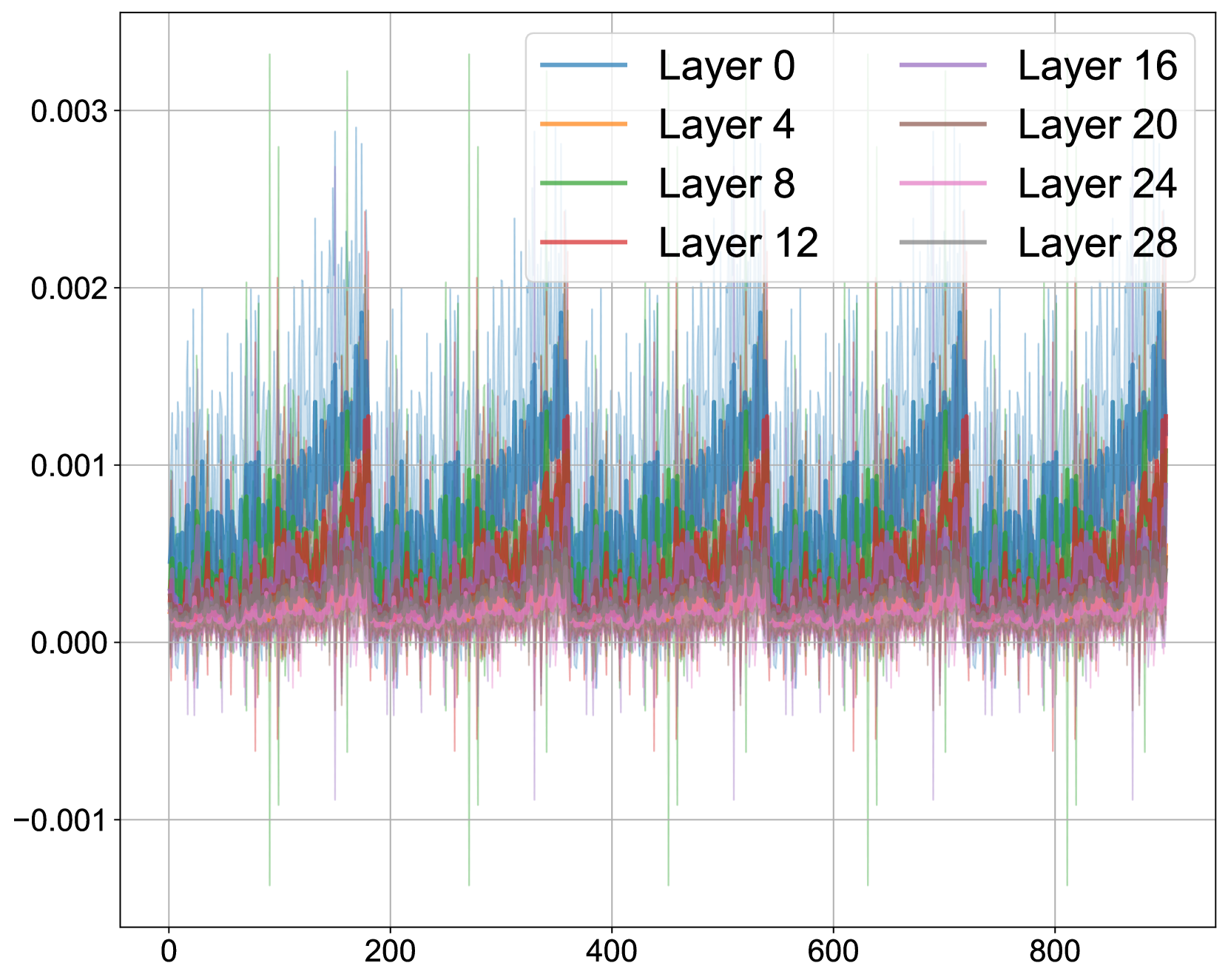
🔼 This figure visualizes the magnitude of key states across different layers of the model and positions within the context. It shows how the magnitude of key states changes as the position in the sequence increases. This visualization helps to understand the impact of position on the attention mechanism and provides insights into the distribution of attention weights across different parts of the context.
read the caption
(b) Key Magnitude

🔼 This figure visualizes the magnitude of value states across different layers and positions within the attention mechanism. It shows how the magnitude of value states changes as the position in the context sequence increases. This is important because the magnitude of value states influences their contribution to the final attention weights, and thus the generation of the model’s output. The plot likely shows a trend or pattern in the value state magnitudes, possibly highlighting areas where the magnitudes are unusually high or low. This could indicate important information or potential areas of misalignment that the authors might analyze further in the paper.
read the caption
(c) Value Magnitude

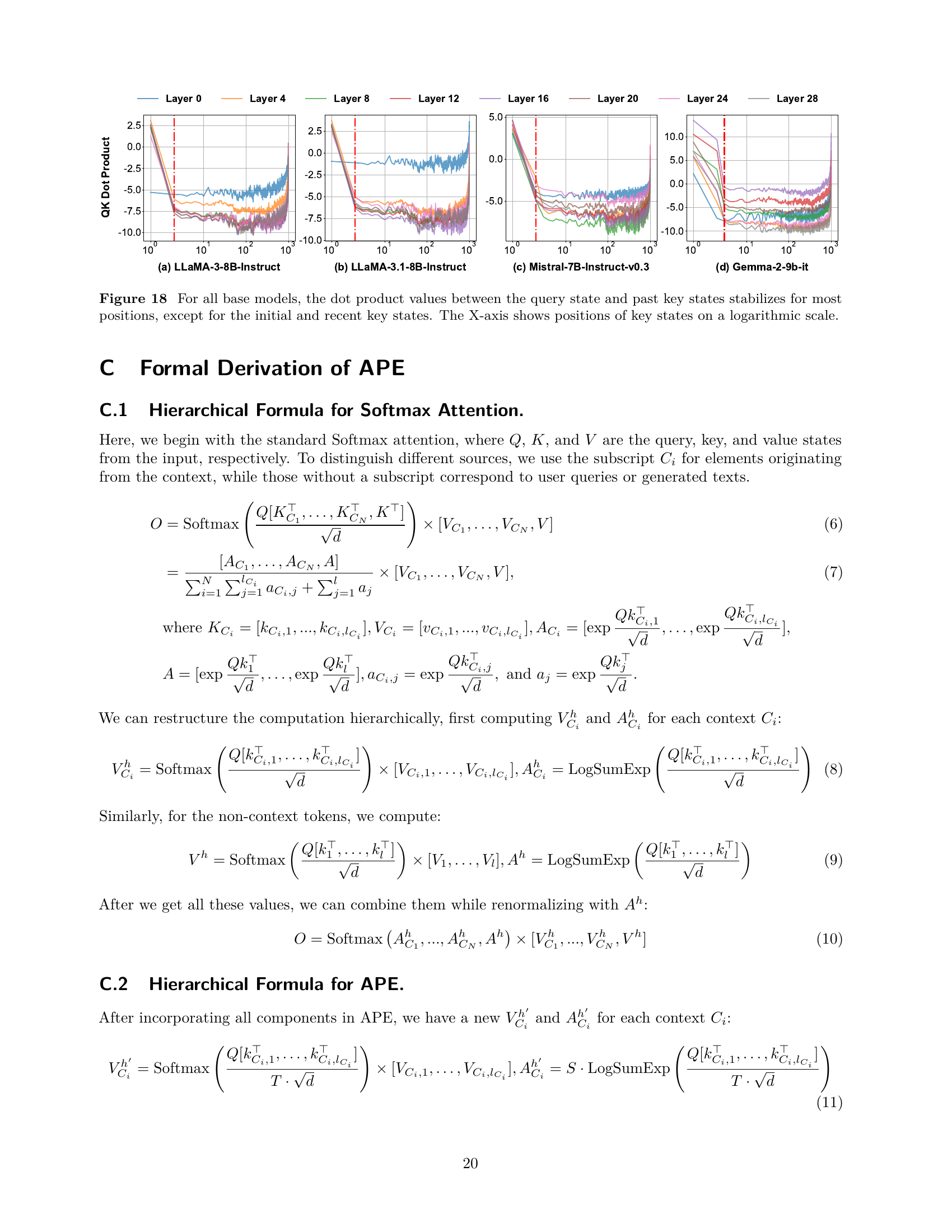
🔼 This figure visualizes the dot product between query and key states across different layers and positions. It shows that the dot products are generally low except for the initial and recent positions, indicating that the attention mechanism focuses more on tokens at the beginning and end of the context. The X-axis represents the position of key states, and the Y-axis represents the query-key dot product.
read the caption
(d) Query-Key Product

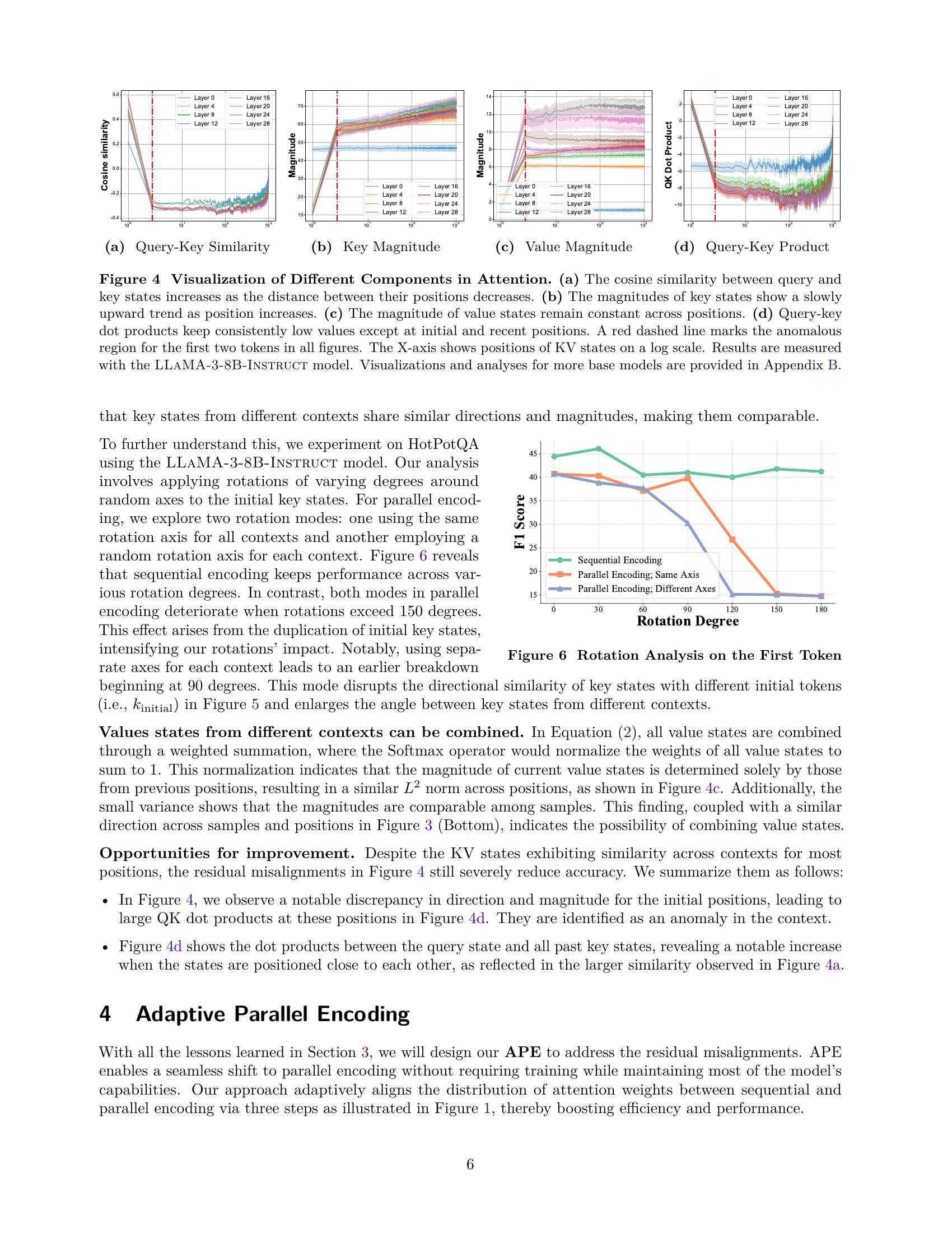
🔼 Figure 4 analyzes the attention mechanism’s behavior in LLMs. Panel (a) shows that the cosine similarity between query and key states is higher for closer positions, indicating stronger attention between nearby tokens. Panel (b) illustrates a gradual increase in the magnitude of key states as position advances. Panel (c) demonstrates that the magnitudes of value states remain relatively stable across all positions. Panel (d) reveals that the query-key dot products generally remain low, with notable exceptions at the beginning and end of the sequence. The red dashed line highlights the first two tokens, which exhibit atypical behavior. The x-axis represents the position of key/value states on a logarithmic scale, and the results are from the LLAMA-3-8B-Instruct model. Appendix B expands on similar visualizations and analysis for other models.
read the caption
Figure 4: Visualization of Different Components in Attention. (a) The cosine similarity between query and key states increases as the distance between their positions decreases. (b) The magnitudes of key states show a slowly upward trend as position increases. (c) The magnitude of value states remain constant across positions. (d) Query-key dot products keep consistently low values except at initial and recent positions. A red dashed line marks the anomalous region for the first two tokens in all figures. The X-axis shows positions of KV states on a log scale. Results are measured with the LLaMA-3-8B-Instruct model. Visualizations and analyses for more base models are provided in Appendix 11.

🔼 This figure visually demonstrates the geometric relationships between key states (vectors) from different contexts in the model. It shows how the angle between key states from different contexts is significantly larger than the angle between an initial key state and its subsequent states within the same context. This observation helps explain why the attention mechanism in LLMs can naturally create alignments between contexts even when they are processed independently in parallel. The similarity in angles indicates that the key states are not randomly oriented but exhibit a directional consistency.
read the caption
Figure 5: Geometry of Key States.
🔼 This figure shows the impact of rotating the initial token’s key states on the model’s performance in both sequential and parallel encoding settings. Different rotation degrees (around random axes) were applied to the initial key states. The x-axis represents the rotation degree, and the y-axis represents the F1 score achieved by the model. The ‘Sequential Encoding’ line serves as a baseline, illustrating the model’s performance without any rotation. The ‘Parallel Encoding; Same Axis’ line shows the results when all contexts use the same rotation axis, while ‘Parallel Encoding; Different Axes’ shows results when each context gets a unique rotation axis. The figure demonstrates that while sequential encoding is robust to rotation, parallel encoding exhibits a significant decrease in performance as the rotation degree increases, indicating a greater sensitivity to changes in initial key state orientation. This highlights the potential misalignment issues in parallel encoding, which APE aims to address.
read the caption
Figure 6: Rotation Analysis on the First Token

🔼 This figure shows the attention weight distribution within contexts for sequential encoding. Sequential encoding allocates high attention scores to tokens that are close together in the input sequence, demonstrating the model’s sensitivity to the immediate context. The x-axis shows the position of tokens. This visualization helps to illustrate the typical behavior of attention mechanisms in sequential models, providing a baseline for comparison with other encoding methods shown in subsequent parts of the figure.
read the caption
(a) Sequential

🔼 Figure 7(b) displays the attention weight distribution within contexts when using parallel encoding with a temperature (T) of 1.0. It illustrates how the attention scores are distributed across tokens within each context. This visualization helps to understand the impact of temperature on the attention mechanism and the differences between sequential and parallel encoding.
read the caption
(b) Parallel (T = 1.0)

🔼 This figure shows the distribution of attention weights within contexts when using parallel encoding with an attention temperature (T) of 0.2. It visually compares this distribution to those shown in Figures 7a and 7b (sequential encoding and parallel encoding with T=1.0, respectively). The x-axis represents the token positions, and the y-axis shows the attention weights. Lowering the temperature (T) to 0.2 makes the distribution sparser, focusing attention on the most relevant tokens. This plot helps to illustrate the effect of adjusting the attention temperature as a step in the Adaptive Parallel Encoding (APE) method to align the attention distribution of parallel encoding with sequential encoding.
read the caption
(c) Parallel (T = 0.2)
🔼 This figure compares the attention weight distribution within contexts between parallel and sequential encoding methods. It shows how the parallel encoding, with its inherent distribution of attention scores among neighboring tokens from all contexts, contrasts with the more focused attention distribution of sequential encoding. In particular, it visualizes how adjusting the temperature in parallel encoding (from T=1.0 to T=0.2) can lead to a more sparse distribution, making it closer to that of sequential encoding.
read the caption
(d) Parallel vs. Sequential

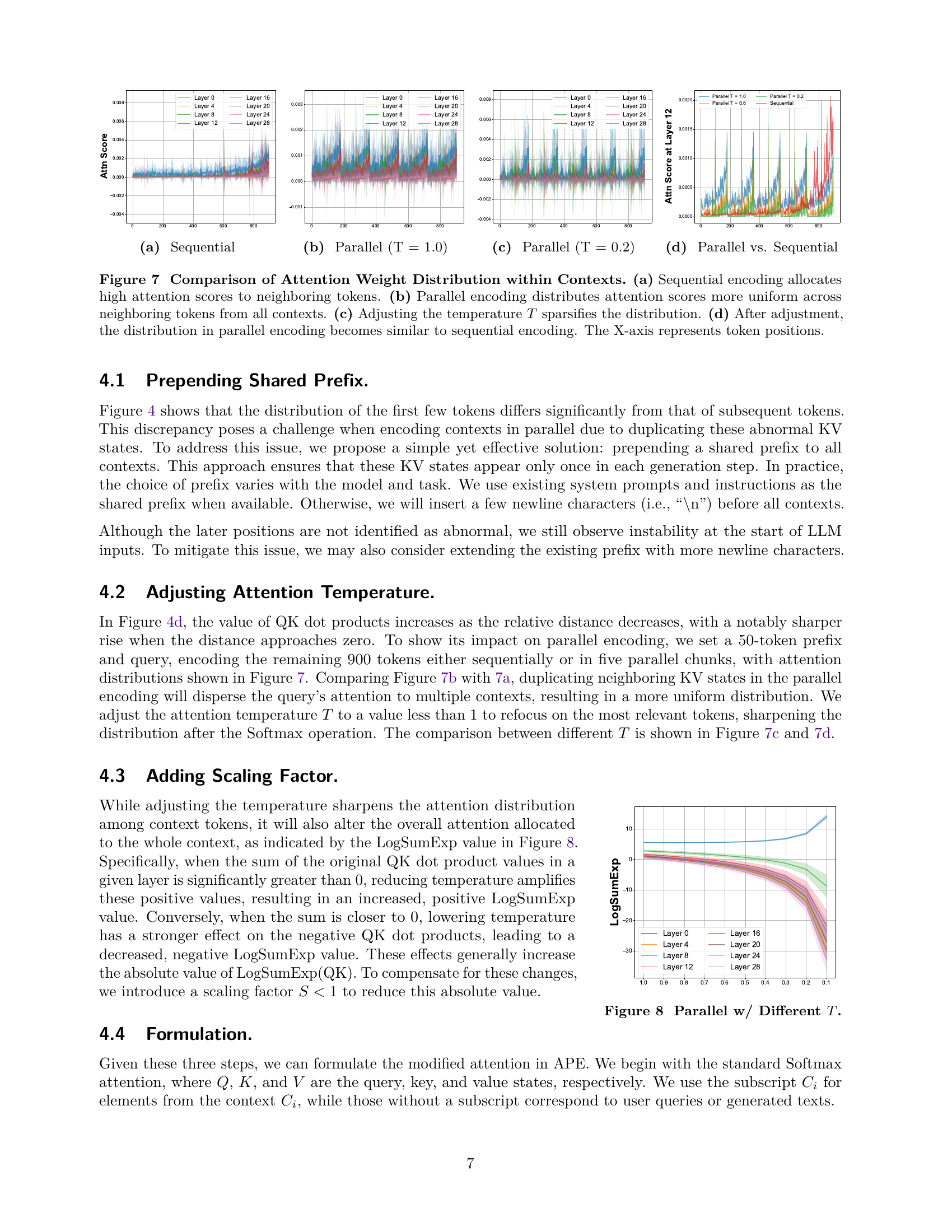
🔼 Figure 7 demonstrates the effects of different encoding methods and temperature adjustments on the distribution of attention weights within contexts. Panel (a) shows that sequential encoding concentrates attention on nearby tokens. In contrast, panel (b) illustrates that parallel encoding distributes attention more uniformly across neighboring tokens from all contexts. Panel (c) demonstrates how lowering the temperature parameter (T) makes the attention distribution sparser. Finally, panel (d) shows that after temperature adjustment, the attention weight distribution in parallel encoding closely resembles that of sequential encoding. The horizontal axis of all subplots represents the position of the tokens.
read the caption
Figure 7: Comparison of Attention Weight Distribution within Contexts. (a) Sequential encoding allocates high attention scores to neighboring tokens. (b) Parallel encoding distributes attention scores more uniform across neighboring tokens from all contexts. (c) Adjusting the temperature T𝑇Titalic_T sparsifies the distribution. (d) After adjustment, the distribution in parallel encoding becomes similar to sequential encoding. The X-axis represents token positions.

🔼 This figure visualizes the effect of different attention temperatures (T) on the LogSumExp value, a key component in the attention mechanism of the Adaptive Parallel Encoding (APE) model. It illustrates how changing the temperature impacts the distribution of attention weights across various layers of the model, specifically showing how the LogSumExp value changes as the temperature parameter is varied from 1.0 to 0.1. Different curves represent the results for distinct layers within the model.
read the caption
Figure 8: Parallel w/ Different T𝑇Titalic_T.

🔼 This figure (Figure 11 in the paper) displays the cosine similarity between key states from different samples in each position across various layers for four different language models. The X-axis represents the positions of key states on a logarithmic scale. The purpose is to visualize the alignment and misalignment between parallel encoding and sequential encoding, highlighting the similarity of key states across different samples, especially in later layers, for LLAMA-3-8B-INSTRUCT, LLAMA-3.1-8B-INSTRUCT, and MISTRAL-7B-INSTRUCT-V0.3. This similarity is strong evidence that parallel encoding can work because of the inherent alignments between KV states from different positions in independent contexts.
read the caption
(a) Llama-3-8B-Instruct

🔼 The figure is a visualization of the cosine similarity between key states from distinct initial tokens in the LLAMA-3.1-8B-Instruct model. The cosine similarity is measured for each layer of the model and plotted against various positions. This graph helps to show the degree of similarity between different samples across positions within the model. This is part of the analysis on how parallel encoding and sequential encoding differ.
read the caption
(b) Llama-3.1-8B-Instruct

🔼 Figure 11 shows the cosine similarity between key states from different initial tokens across various layers for the Mistral-7B-Instruct-v0.3 model. The x-axis represents the position of key states on a logarithmic scale. The high cosine similarity values, particularly above 0.8, demonstrate a strong alignment between key states from different initial tokens for most layers and positions, especially in the later layers. This indicates the key states of independent contexts are quite similar, which provides evidence supporting the effectiveness of parallel encoding in this model.
read the caption
(c) Mistral-7B-Instruct-v0.3

🔼 Figure 11(d) presents a visualization of cosine similarity between key states from different samples in each position for the GEMMA-2-9B-IT language model. The figure shows a graph plotting cosine similarity against position (log scale). The graph displays the results for eight different layers in the model. This visualization aims to highlight the degree of similarity between key state vectors from different model instances, providing insights into the stability and consistency of these vectors at various positions within the sequence. The similarity between key states across various model instances shows how well the parallel encoding method maintains the positional information during the pre-computation of KV states.
read the caption
(d) Gemma-2-9b-it

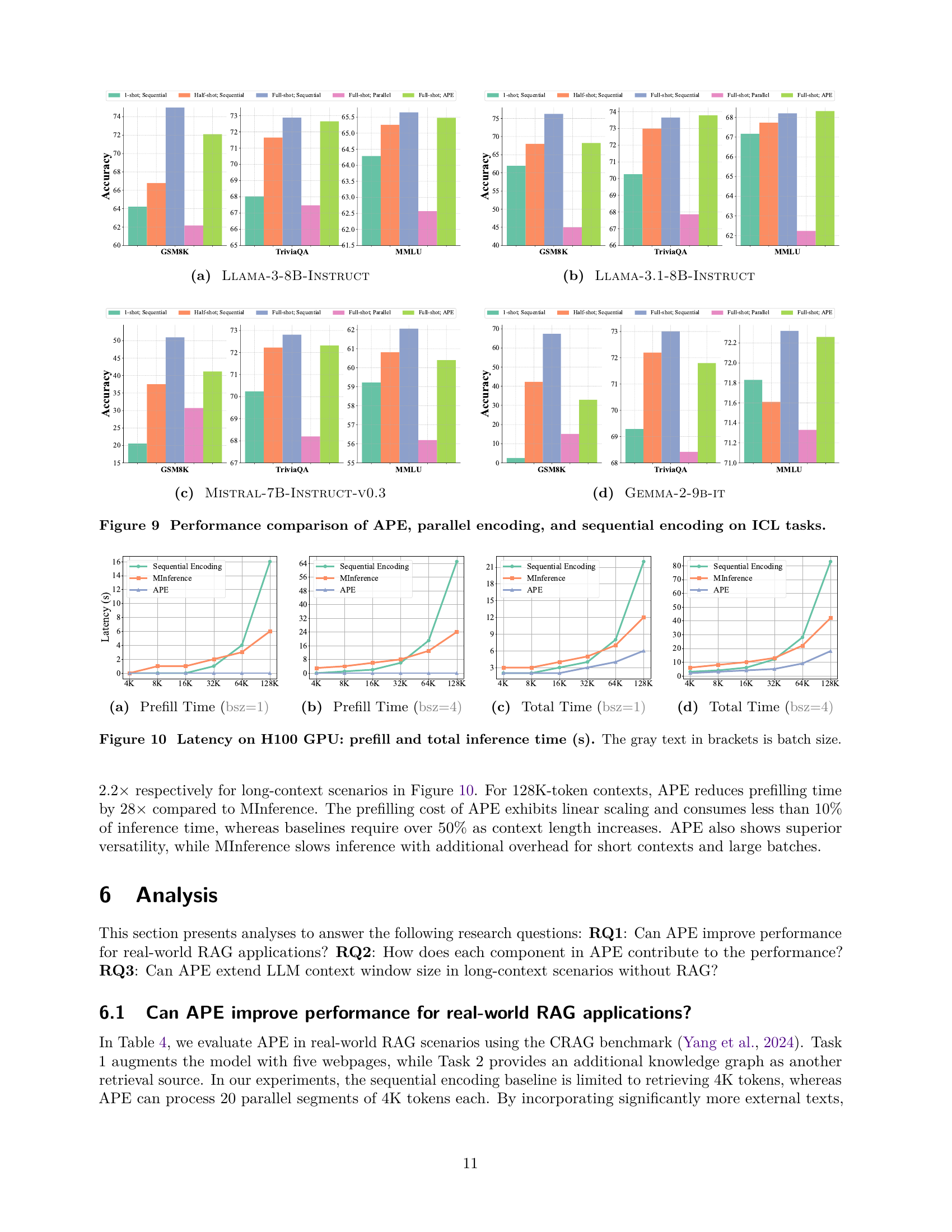
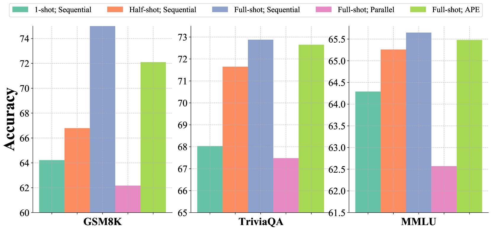
🔼 This figure presents a comparison of the performance of three different context encoding methods on In-Context Learning (ICL) tasks. The methods compared are Adaptive Parallel Encoding (APE), parallel encoding, and sequential encoding. The performance is evaluated across multiple ICL tasks using different language models (LLaMA-3-8B-INSTRUCT, LLaMA-3.1-8B-INSTRUCT, MISTRAL-7B-INSTRUCT-v0.3, and GEMMA-2-9B-IT) and varying numbers of shots (1-shot, half-shot, and full-shot). The results are displayed in terms of accuracy, highlighting the relative strengths and weaknesses of each encoding method in different ICL scenarios.
read the caption
Figure 9: Performance comparison of APE, parallel encoding, and sequential encoding on ICL tasks.
🔼 This figure shows the time taken to pre-process (prefill) the context for a given model before generating text. The experiment is run with a batch size of 1. The x-axis represents the length of context (in tokens), ranging from 4K to 128K. The y-axis represents the prefilling time in seconds. Multiple lines represent different methods used for pre-processing: Sequential Encoding, MInference, and APE (Adaptive Parallel Encoding). Comparing the lines shows how APE performs against these other methods in terms of speed of context pre-processing.
read the caption
(a) Prefill Time (bsz=1)

🔼 This figure shows the prefilling time taken for different context lengths (4K, 8K, 16K, 32K, 64K, and 128K tokens) using a batch size of 4. The prefilling time is the time it takes to prepare the context (key-value states) before the model can start generating text in response to a user query. The figure compares the prefilling times of three different encoding methods: Sequential encoding, MInference, and APE (Adaptive Parallel Encoding). By comparing these methods across various context lengths, we can understand the efficiency gains of APE, particularly for longer contexts.
read the caption
(b) Prefill Time (bsz=4)
🔼 This figure shows the total inference time taken for different context lengths using a batch size of 1. The total time encompasses both the time to pre-fill the context and the time to generate the response. It compares the performance of sequential encoding, MInference, and APE (Adaptive Parallel Encoding). The x-axis represents the context length, and the y-axis represents the total inference time in seconds.
read the caption
(c) Total Time (bsz=1)

🔼 This figure displays the total inference time taken for different context lengths (4K, 8K, 16K, 32K, 64K, and 128K tokens) when using a batch size of 4. The total time includes both the time to prefill the context and the time to generate the response. It compares the performance of sequential encoding, MInference, and APE, illustrating the time efficiency gains achieved by APE across varying context lengths.
read the caption
(d) Total Time (bsz=4)

🔼 This figure presents a performance comparison of different context encoding methods on the task of generating text from a long context. Specifically, it shows the time taken for context pre-filling (preparing the necessary context information) and the total inference time (time to generate the text after pre-filling) for sequential encoding (the traditional method), MInference (an optimized method), and APE (the proposed method). The experiments were run on a H100 GPU with batch sizes of 1 and 4, and various context lengths are tested. The results show that APE significantly reduces both pre-filling time and total inference time compared to sequential encoding and MInference, demonstrating the effectiveness of the proposed method.
read the caption
Figure 10: Latency on H100 GPU: prefill and total inference time (s). The gray text in brackets is batch size.

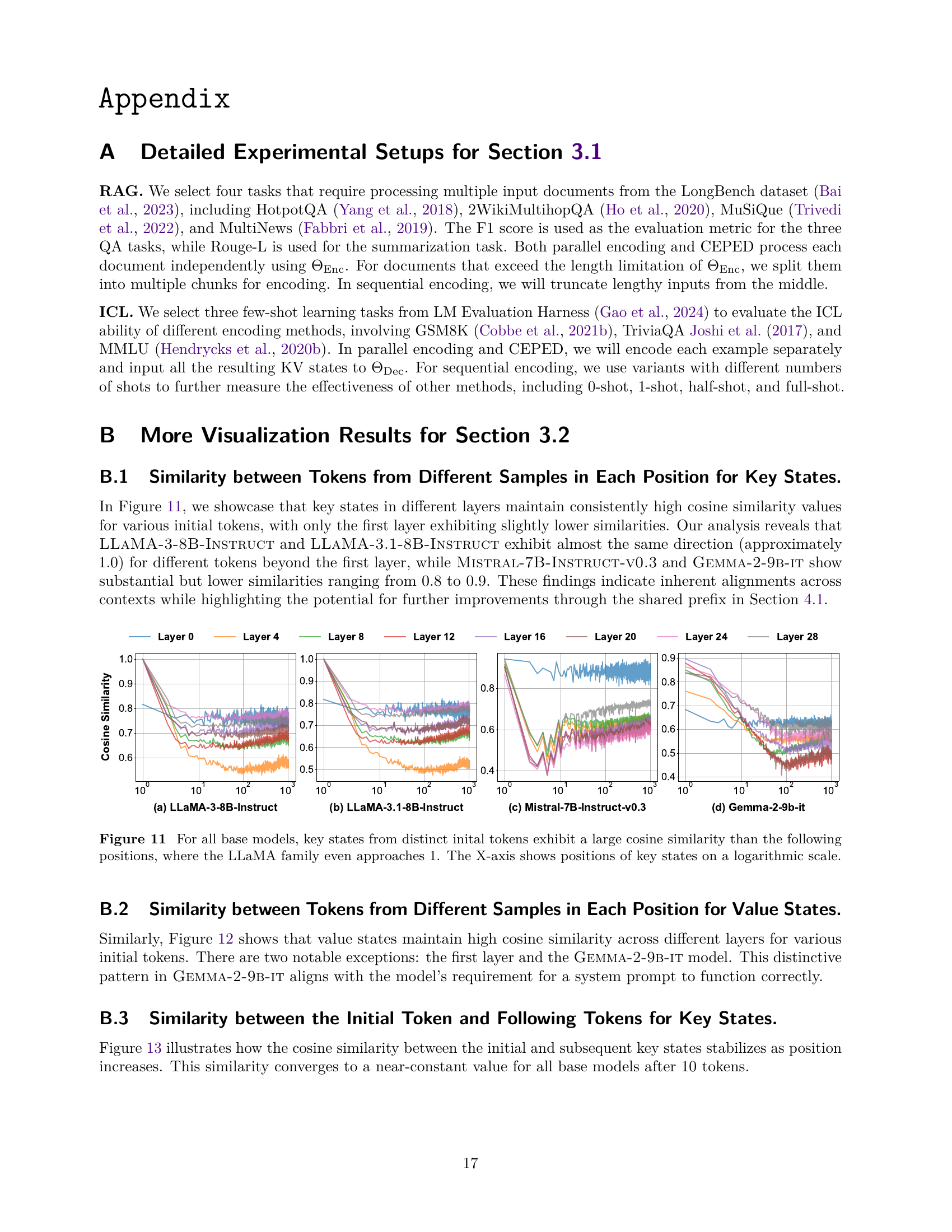
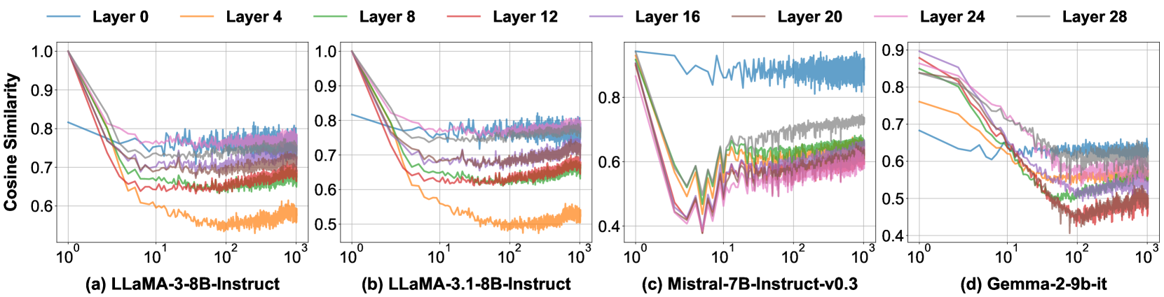
🔼 This figure displays the cosine similarity between key states from different initial tokens across various layers and positions within the model. A high cosine similarity indicates that the key states from different samples have similar directions in vector space. The observation that cosine similarity is higher for initial tokens compared to later tokens within the same layer suggests a consistent attention pattern. LLaMA models show near-perfect similarity (approaching 1.0), while other models exhibit strong but not as high similarity (ranging from 0.8 to 0.9). The x-axis displays the position of the key states on a logarithmic scale, allowing a clear visualization of the similarity patterns across various positions.
read the caption
Figure 11: For all base models, key states from distinct inital tokens exhibit a large cosine similarity than the following positions, where the LLaMA family even approaches 1. The X-axis shows positions of key states on a logarithmic scale.

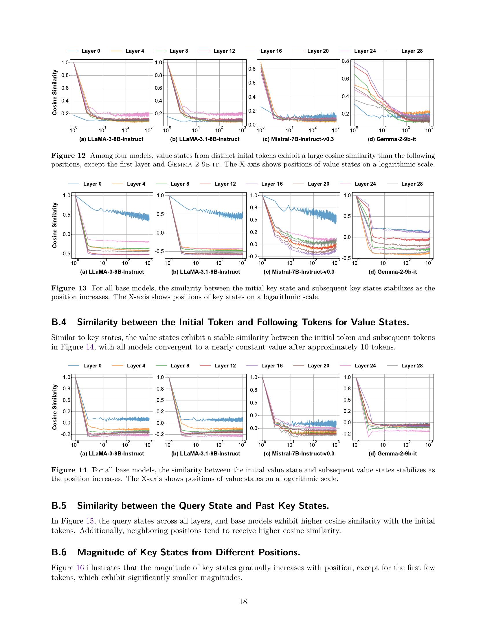
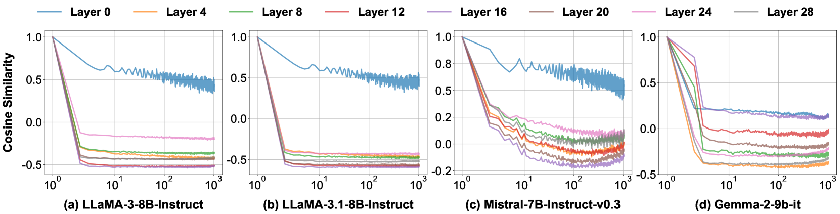
🔼 This figure visualizes the cosine similarity between value states from different initial tokens across various layers and positions within four large language models (LLMs): LLAMA-3-8B-Instruct, LLAMA-3.1-8B-Instruct, Mistral-7B-Instruct-v0.3, and Gemma-2-9B-it. The x-axis represents the position of value states on a logarithmic scale, illustrating how the similarity changes as the position moves away from the initial token. Notably, the plot shows that the cosine similarity between value states of distinct initial tokens is generally high across various layers, except for the first layer and the Gemma-2-9B-it model, indicating a strong similarity in direction and magnitude of value states from different contexts. This observation supports the claim that value states from different contexts can be effectively combined without substantial loss of information.
read the caption
Figure 12: Among four models, value states from distinct inital tokens exhibit a large cosine similarity than the following positions, except the first layer and Gemma-2-9b-it. The X-axis shows positions of value states on a logarithmic scale.

🔼 This figure displays the cosine similarity between the initial key state and subsequent key states across various positions for four different large language models (LLMs). The cosine similarity is calculated to measure the similarity in direction and magnitude of the key states across different positions within the same context. The x-axis represents position on a logarithmic scale, illustrating how quickly the similarity stabilizes for each model, which indicates the consistency of the key state directions within a context. The y-axis represents the cosine similarity value.
read the caption
Figure 13: For all base models, the similarity between the initial key state and subsequent key states stabilizes as the position increases. The X-axis shows positions of key states on a logarithmic scale.

🔼 This figure visualizes the cosine similarity between the initial value state and subsequent value states across different positions within a sequence for four large language models (LLMs). The x-axis represents the position of the value state on a logarithmic scale, while the y-axis represents the cosine similarity. The results show that across all four models, this cosine similarity converges to a nearly constant value after approximately ten tokens. The figure helps demonstrate the stability and consistency of value state representations in LLMs, particularly after the initial few states which exhibit more variation.
read the caption
Figure 14: For all base models, the similarity between the initial value state and subsequent value states stabilizes as the position increases. The X-axis shows positions of value states on a logarithmic scale.

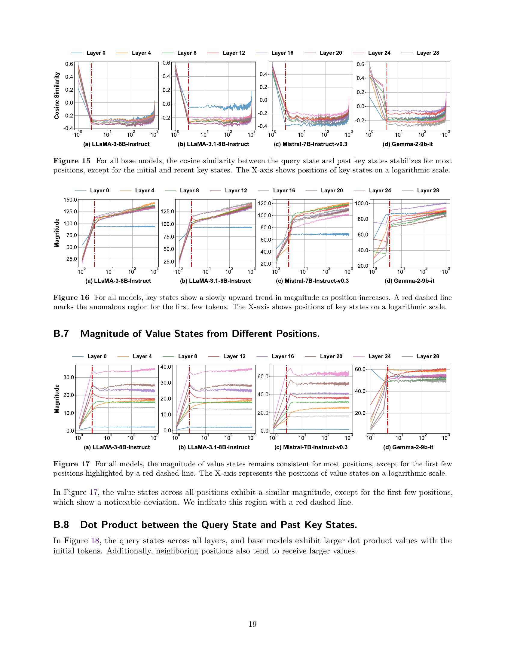
🔼 This figure visualizes the cosine similarity between the query state and previous key states across different layers and base models. The x-axis represents the positions of key states, plotted on a logarithmic scale. The results show that cosine similarity generally stabilizes for most positions. However, there are notable exceptions at the initial and most recent positions, indicating that these positions have higher attention weights compared to other positions.
read the caption
Figure 15: For all base models, the cosine similarity between the query state and past key states stabilizes for most positions, except for the initial and recent key states. The X-axis shows positions of key states on a logarithmic scale.
More on tables
| Model | MuSiQue | Qasper | 2WikiMQA | DuRead | HotpotQA | NarratQA | MFQA_zh | MFQA_en | Avg. |
|---|---|---|---|---|---|---|---|---|---|
| LLaMA-3-8B-Instruct | 20.70 | 41.05 | 30.02 | 9.55 | 45.90 | 20.98 | 58.54 | 45.04 | 33.97 |
| C200×20, Sequential | 27.93 | 42.71 | 38.35 | 12.65 | 49.60 | 22.78 | 57.82 | 48.94 | 37.60 |
| C4000×20, PCW | 18.82 | 42.59 | 40.99 | 21.57 | 47.09 | 23.29 | 54.40 | 45.05 | 36.73 |
| C4000×20, APE | 26.19 | 42.32 | 44.43 | 23.13 | 49.71 | 30.71 | 55.03 | 45.41 | 39.62 |
| Mistral-7B-Instruct-v0.3 | 10.05 | 31.08 | 22.12 | 17.68 | 32.09 | 19.68 | 32.03 | 40.38 | 25.64 |
| C200×20, Sequential | 11.58 | 21.98 | 24.44 | 20.80 | 32.79 | 16.06 | 34.43 | 38.40 | 25.06 |
| C4000×20, PCW | 17.58 | 35.57 | 32.97 | 18.70 | 37.05 | 14.10 | 34.69 | 40.14 | 28.85 |
| C4000×20, APE | 20.30 | 36.81 | 34.37 | 21.89 | 42.33 | 20.49 | 40.20 | 44.03 | 32.55 |
| Gemma-2-9b-it | 22.57 | 39.99 | 48.06 | 27.40 | 47.49 | 23.11 | 50.81 | 45.35 | 38.10 |
| C200×10, Sequential | 30.69 | 42.86 | 53.55 | 28.04 | 52.05 | 24.45 | 50.25 | 48.34 | 41.28 |
| C2000×20, PCW | 26.27 | 46.69 | 47.59 | 23.43 | 48.95 | 27.11 | 56.69 | 49.81 | 40.82 |
| C2000×20, APE | 33.38 | 47.72 | 49.49 | 28.43 | 56.62 | 30.41 | 56.52 | 50.84 | 44.18 |
| LLaMA-3.1-8B-Instruct | 22.18 | 46.81 | 40.58 | 34.61 | 43.97 | 23.08 | 61.60 | 51.89 | 38.98 |
| 128K, Sequential | 28.35 | 47.20 | 40.81 | 33.34 | 53.46 | 30.57 | 61.97 | 53.25 | 42.24 |
| C200×20, Sequential | 30.62 | 42.33 | 44.39 | 33.51 | 49.97 | 23.87 | 56.87 | 55.14 | 40.22 |
| C4000×20, PCW | 21.23 | 41.52 | 44.87 | 31.11 | 49.47 | 19.98 | 60.90 | 51.19 | 38.44 |
| C4000×20, APE | 26.88 | 43.03 | 50.11 | 32.10 | 55.41 | 30.50 | 62.02 | 52.51 | 42.86 |
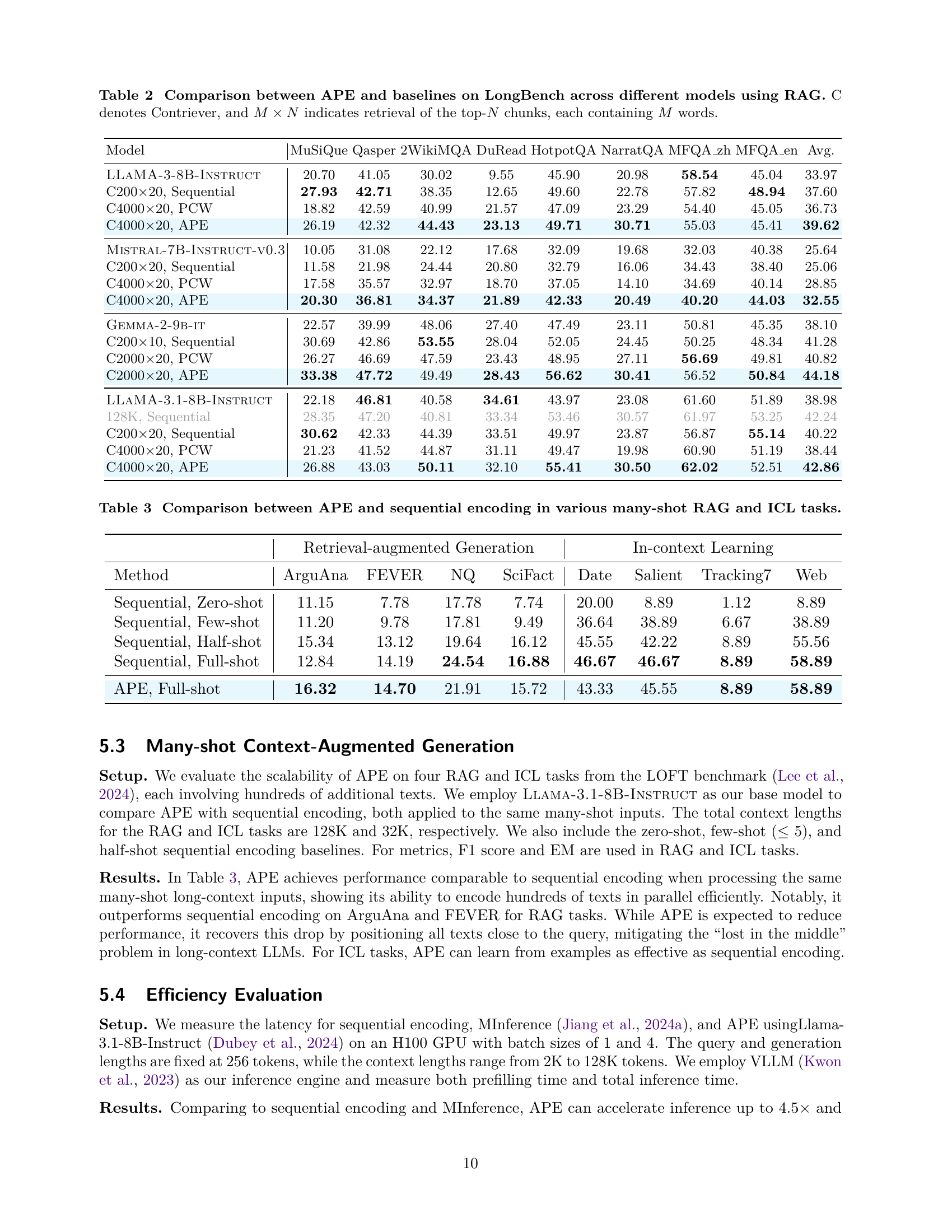
🔼 Table 2 presents a comparison of APE’s performance against various baselines on the LongBench benchmark. The experiment uses Retrieval Augmented Generation (RAG) with different models. The table shows results for different numbers of retrieved contexts (M) and the top N retrieved contexts. The baselines include sequential encoding (without RAG), parallel context windows (PCW), and APE. The performance is evaluated across several different tasks within the LongBench benchmark. Each task’s results are shown for each model, along with the average performance across all models.
read the caption
Table 2: Comparison between APE and baselines on LongBench across different models using RAG. C denotes Contriever, and M×N𝑀𝑁M\times Nitalic_M × italic_N indicates retrieval of the top-N𝑁Nitalic_N chunks, each containing M𝑀Mitalic_M words.
| Retrieval-augmented Generation | In-context Learning | |||||||
|---|---|---|---|---|---|---|---|---|
| Method | ArguAna | FEVER | NQ | SciFact | Date | Salient | Tracking7 | Web |
| Sequential, Zero-shot | 11.15 | 7.78 | 17.78 | 7.74 | 20.00 | 8.89 | 1.12 | 8.89 |
| Sequential, Few-shot | 11.20 | 9.78 | 17.81 | 9.49 | 36.64 | 38.89 | 6.67 | 38.89 |
| Sequential, Half-shot | 15.34 | 13.12 | 19.64 | 16.12 | 45.55 | 42.22 | 8.89 | 55.56 |
| Sequential, Full-shot | 12.84 | 14.19 | 24.54 | 16.88 | 46.67 | 46.67 | 8.89 | 58.89 |
| APE, Full-shot | 16.32 | 14.70 | 21.91 | 15.72 | 43.33 | 45.55 | 8.89 | 58.89 |
🔼 This table presents a comparison of the performance of Adaptive Parallel Encoding (APE) against sequential encoding in various scenarios involving many contexts for both Retrieval Augmented Generation (RAG) and In-context Learning (ICL). It shows how APE handles multiple contexts in parallel and compares its accuracy to the standard method, offering insights into its effectiveness in diverse, complex tasks.
read the caption
Table 3: Comparison between APE and sequential encoding in various many-shot RAG and ICL tasks.
| Task | Model | Latency (ms) | Accuracy (%) | Hallucination | Missing | Scorea |
|---|---|---|---|---|---|---|
| LLM only | Llama-3-8B-Instruct | 682 | 22.14 | 48.97 | 28.90 | -26.83 |
| Task 1 | Llama-3-8B-Instruct | 1140 | 23.28 | 29.49 | 47.22 | -6.21 |
| +APE | 1054 | 25.53 | 21.30 | 37.93 | -0.41 | |
| Task 2 | Llama-3-8B-Instruct | 1830 | 24.46 | 28.38 | 47.15 | -3.92 |
| +APE | 1672 | 27.04 | 18.74 | 37.32 | 2.16 |
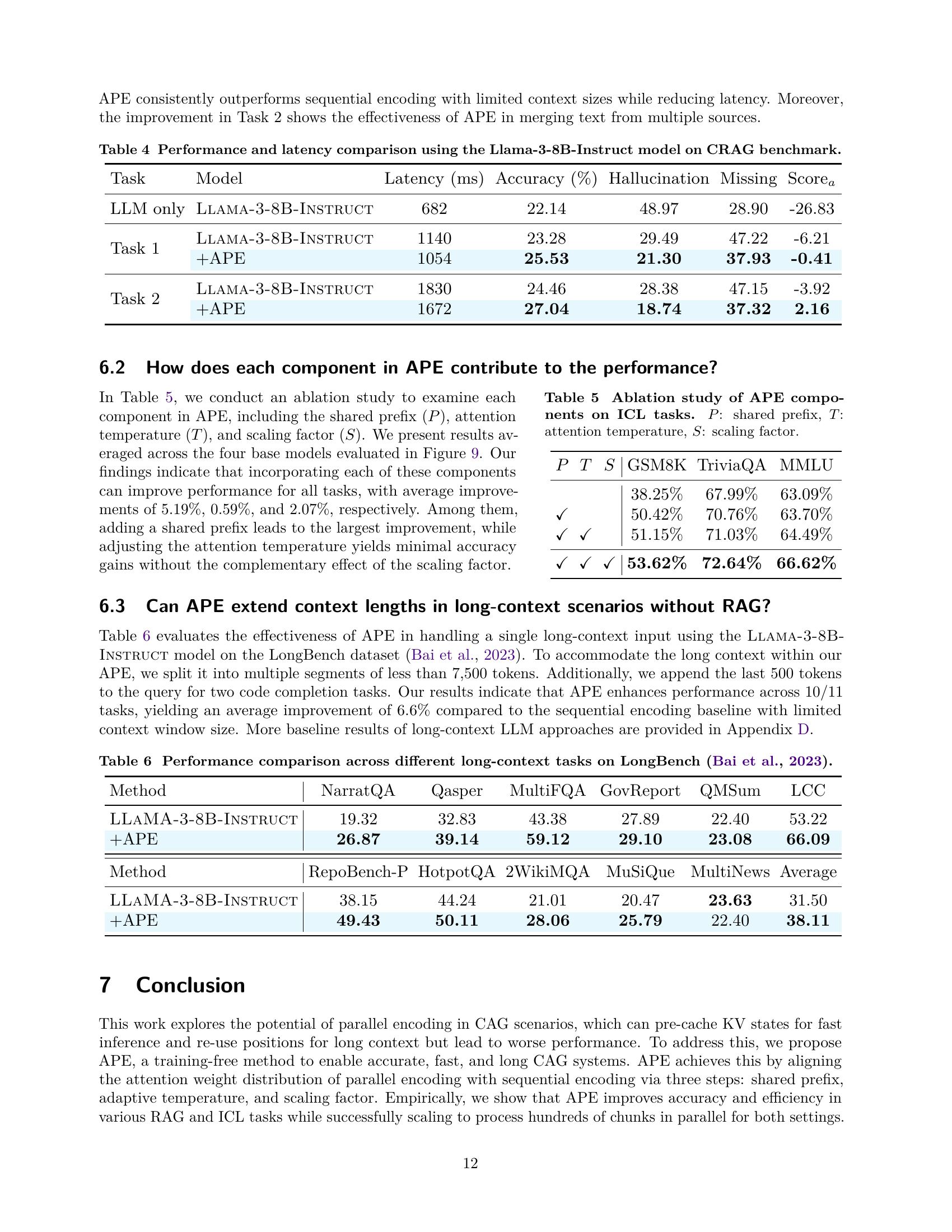
🔼 This table presents a comparison of performance and latency between the Llama-3-8B-Instruct model alone and when augmented with APE on the CRAG benchmark. It shows the accuracy, hallucination rate, and missing score for two different tasks. Task 1 uses only webpages as additional context, while Task 2 incorporates both webpages and a knowledge graph. The table aims to demonstrate APE’s ability to improve performance and reduce latency in real-world RAG applications.
read the caption
Table 4: Performance and latency comparison using the Llama-3-8B-Instruct model on CRAG benchmark.
| GSM8K | TriviaQA | MMLU | |||
|---|---|---|---|---|---|
| 38.25% | 67.99% | 63.09% | |||
| ✓ | 50.42% | 70.76% | 63.70% | ||
| ✓ | ✓ | 51.15% | 71.03% | 64.49% | |
| ✓ | ✓ | ✓ | 53.62% | 72.64% | 66.62% |
🔼 This table presents an ablation study analyzing the impact of each component in the Adaptive Parallel Encoding (APE) method on the performance of in-context learning (ICL) tasks. It shows the effectiveness of the shared prefix (P), attention temperature (T), and scaling factor (S) individually and in combination, demonstrating their contribution to the overall accuracy improvement achieved by APE. The results are presented as average performance across multiple ICL tasks and multiple base models, facilitating a clear understanding of the relative significance of each component.
read the caption
Table 5: Ablation study of APE components on ICL tasks. P𝑃Pitalic_P: shared prefix, T𝑇Titalic_T: attention temperature, S𝑆Sitalic_S: scaling factor.
| Method | NarratQA | Qasper | MultiFQA | GovReport | QMSum | LCC |
|---|---|---|---|---|---|---|
| LLaMA-3-8B-Instruct | 19.32 | 32.83 | 43.38 | 27.89 | 22.40 | 53.22 |
| +APE | 26.87 | 39.14 | 59.12 | 29.10 | 23.08 | 66.09 |
| Method | RepoBench-P | HotpotQA | 2WikiMQA | MuSiQue | MultiNews | Average |
| LLaMA-3-8B-Instruct | 38.15 | 44.24 | 21.01 | 20.47 | 23.63 | 31.50 |
| +APE | 49.43 | 50.11 | 28.06 | 25.79 | 22.40 | 38.11 |
🔼 This table presents a comparison of the performance of APE against various baselines on LongBench, a benchmark dataset for evaluating long-context capabilities in large language models. The results are shown across eleven different tasks, indicating the accuracy achieved by each method on each task. The baselines include sequential encoding, and other competitive approaches. This allows for a comprehensive assessment of APE’s effectiveness in handling long-context inputs.
read the caption
Table 6: Performance comparison across different long-context tasks on LongBench (Bai et al., 2023).
| Method | NarratQA | Qasper | MultiFQA | GovReport | QMSum | LCC |
|---|---|---|---|---|---|---|
| LLaMA-3-8B-Instruct | 19.32 | 32.83 | 43.38 | 27.89 | 22.40 | 53.22 |
| LLMLingua2 | 21.00 | 25.78 | 48.92 | 27.09 | 22.34 | 16.41 |
| StreamingLLM | 16.99 | 28.94 | 11.99 | 25.65 | 19.91 | 40.02 |
| Long-context FT | 14.88 | 21.70 | 47.79 | 32.65 | 24.76 | 55.12 |
| Self-Extend | 24.82 | 37.94 | 50.99 | 30.48 | 23.36 | 58.01 |
| +APE | 26.87 | 39.14 | 59.12 | 29.10 | 23.08 | 66.09 |
| Method | RepoBench-P | HotpotQA | 2WikiMQA | MuSiQue | MultiNews | Average |
| LLaMA-3-8B-Instruct | 38.15 | 44.24 | 21.01 | 20.47 | 23.63 | 31.50 |
| LLMLingua2 | 20.56 | 40.16 | 24.72 | 20.85 | 21.34 | 26.29 |
| StreamingLLM | 26.16 | 32.76 | 20.12 | 17.32 | 21.49 | 23.76 |
| Long-context FT | 43.05 | 15.89 | 10.49 | 8.74 | 24.28 | 27.21 |
| Self-Extend | 41.83 | 51.09 | 24.17 | 28.73 | 24.11 | 35.96 |
| +APE | 49.43 | 50.11 | 28.06 | 25.79 | 22.40 | 38.11 |
🔼 This table presents a performance comparison between the proposed Adaptive Parallel Encoding (APE) method and several existing long-context Large Language Models (LLMs) on the LongBench benchmark dataset. The comparison is done across multiple tasks, illustrating APE’s performance relative to methods that address long context limitations through different techniques (such as truncation, KV caching, and fine-tuning). Metrics used likely include accuracy or F1 scores on the various LongBench tasks. The aim is to demonstrate APE’s competitiveness and potential advantages.
read the caption
Table 7: Performance comparison between APE and long-context LLMs on LongBench (Bai et al., 2023).
Full paper#