TL;DR#
Large Language Models (LLMs) struggle with many reasoning tasks due to limited training data. Existing methods mainly focus on narrow skills like math or code generation. This research highlights the challenge of scarce and fragmented training data for diverse reasoning tasks in domains such as logical deduction, scientific inference, and symbolic reasoning.
The paper proposes CODEI/O, a novel approach that addresses data scarcity by leveraging the reasoning patterns inherent in code. It transforms code into an input-output prediction format, training LLMs to predict inputs/outputs given code and test cases in natural language. This exposes models to reasoning primitives like logic flow planning, state-space searching etc. The resulting CODEI/O dataset significantly enhances LLM performance across symbolic, scientific, logic, math, and commonsense reasoning tasks. A refined version, CODEI/O++, further improves performance through multi-turn revision of predictions.
Key Takeaways#
Why does it matter?#
This paper is important because it introduces a novel approach to improve the reasoning capabilities of large language models (LLMs) by leveraging the rich reasoning patterns embedded in real-world code. The CODEI/O method is highly scalable, requiring minimal additional data collection, making it relevant to researchers facing data scarcity challenges. The findings also open new avenues for research, investigating the interaction between code and reasoning, as well as optimizing training methods for improved LLM reasoning abilities.
Visual Insights#

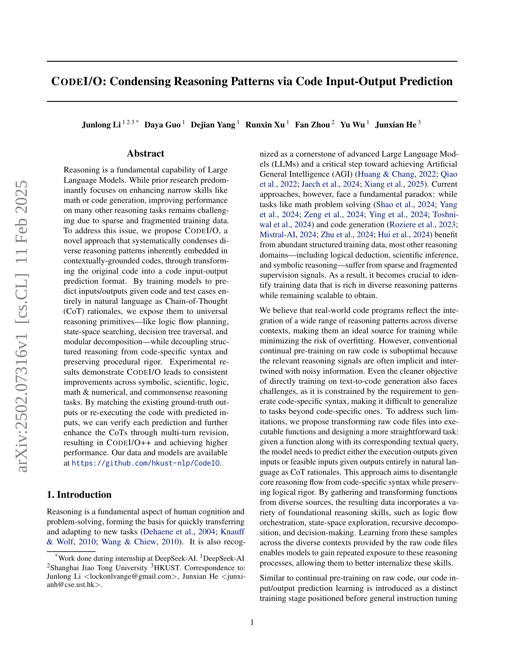
🔼 The figure illustrates the process of creating the training dataset for CODEI/O. It starts with gathering raw code files from diverse sources. These files are then processed and transformed into a standardized format. Next, input and output pairs are generated by executing the code. Simultaneously, natural language Chain-of-Thought (CoT) reasoning is obtained from the DeepSeek-V2.5 model to explain these input-output predictions. Finally, the CoTs are verified and optionally revised to improve the reasoning process. This iterative refinement step helps improve the quality of the training data.
read the caption
Figure 1: Overview of our training data construction: Raw code files are gathered from various sources and converted into a unified format. Input-output pairs are then generated by executing the code, while natural language CoTs for predictions are collected from DeepSeek-V2.5. The verified CoTs can undergo optional revisions to further enhance reasoning chains.
| 1st Stage | Wino | DROP | GSM | MATH | GPQA | MMLU | LC | CRUX | BBH | Zebra | Kor | Live | AVG | |||
|---|---|---|---|---|---|---|---|---|---|---|---|---|---|---|---|---|
| Dataset | # (M) | Grande | 8K | -STEM | -O | -I | -O | -EN | -ZH | Logic | Bench | Bench | ||||
| Qwen 2.5 Coder 7B | ||||||||||||||||
| 2nd Stage Only | 66.9 | 70.7 | 83.4 | 71.6 | 41.5 | 77.2 | 20.7 | 61.3 | 60.0 | 68.3 | 70.6 | 10.9 | 38.7 | 26.0 | 54.8 | |
| WI | 3.5 | 66.3 | 73.5 | 87.0 | 71.4 | 39.1 | 77.5 | 18.3 | 59.1 | 61.6 | 68.6 | 68.7 | 10.2 | 42.5 | 26.0 | 55.0 |
| WI (Full) | 11.6 | 67.0 | 75.0 | 87.0 | 71.1 | 42.9 | 78.6 | 19.1 | 59.3 | 59.8 | 68.4 | 70.4 | 10.9 | 41.9 | 27.6 | 55.6 |
| OMI2 | 3.5 | 67.6 | 74.3 | 84.1 | 72.3 | 36.2 | 77.4 | 20.9 | 60.4 | 61.5 | 68.8 | 69.3 | 10.1 | 42.7 | 27.2 | 55.2 |
| OMI2 (Full) | 14.0 | 66.9 | 74.0 | 88.5 | 73.2 | 40.9 | 77.8 | 19.9 | 59.5 | 62.4 | 68.3 | 71.3 | 11.2 | 41.2 | 28.4 | 56.0 |
| OC-SFT-1 | 4.2 | 66.6 | 75.3 | 86.7 | 70.9 | 37.7 | 78.0 | 20.3 | 60.9 | 60.1 | 67.5 | 67.6 | 10.8 | 40.1 | 27.5 | 55.0 |
| PyEdu | 7.7 | 66.7 | 74.8 | 85.8 | 71.4 | 40.9 | 77.4 | 19.1 | 58.9 | 62.4 | 67.8 | 65.7 | 10.6 | 39.3 | 25.8 | 54.8 |
| CodeI/O | 3.5 | 67.9 | 76.4 | 86.4 | 71.9 | 43.3 | 77.3 | 23.7 | 63.6 | 64.9 | 69.3 | 72.8 | 10.7 | 44.3 | 28.5 | 57.2 |
| CodeI/O++ | 3.5 | 66.9 | 79.1 | 85.7 | 72.1 | 40.6 | 77.9 | 24.2 | 62.5 | 67.9 | 71.0 | 74.2 | 10.7 | 45.7 | 29.1 | 57.7 |
| LLaMA 3.1 8B | ||||||||||||||||
| 2nd Stage Only | 71.3 | 73.1 | 83.2 | 49.9 | 40.6 | 70.0 | 4.1 | 44.5 | 46.9 | 65.8 | 65.6 | 9.8 | 39.8 | 25.7 | 49.3 | |
| WI | 3.5 | 72.1 | 76.3 | 82.8 | 52.8 | 42.9 | 69.6 | 4.1 | 44.0 | 44.8 | 64.5 | 67.8 | 10.0 | 42.7 | 23.1 | 49.8 |
| OMI2 | 3.5 | 72.2 | 74.8 | 86.2 | 58.9 | 38.2 | 70.1 | 5.8 | 46.1 | 46.4 | 67.4 | 68.6 | 9.5 | 40.3 | 24.5 | 50.6 |
| OC-SFT-1 | 4.2 | 71.0 | 71.9 | 81.8 | 51.1 | 38.2 | 68.4 | 5.7 | 43.5 | 44.9 | 65.6 | 67.6 | 10.5 | 42.0 | 24.7 | 49.1 |
| PyEdu | 7.7 | 70.6 | 69.6 | 83.2 | 49.8 | 42.4 | 69.1 | 5.2 | 43.1 | 44.5 | 64.0 | 65.6 | 10.2 | 42.6 | 25.7 | 49.0 |
| CodeI/O | 3.5 | 71.7 | 73.9 | 83.6 | 53.8 | 43.5 | 69.0 | 9.3 | 50.1 | 53.3 | 67.5 | 65.3 | 10.4 | 40.9 | 24.7 | 51.2 |
| CodeI/O++ | 3.5 | 71.8 | 75.1 | 84.0 | 53.2 | 40.9 | 68.4 | 10.0 | 50.4 | 53.1 | 70.0 | 70.6 | 10.5 | 43.2 | 28.1 | 52.1 |
| DeepSeek Coder v2 Lite 16B | ||||||||||||||||
| 2nd Stage Only | 68.4 | 73.4 | 82.5 | 60.0 | 38.6 | 68.5 | 14.8 | 53.0 | 54.9 | 61.1 | 69.2 | 6.7 | 44.7 | 26.6 | 51.6 | |
| WI | 3.5 | 68.5 | 73.8 | 83.7 | 60.5 | 39.5 | 68.7 | 14.3 | 53.5 | 57.1 | 61.6 | 65.7 | 6.9 | 43.1 | 25.4 | 51.6 |
| OMI2 | 3.5 | 67.6 | 74.1 | 84.7 | 64.7 | 38.4 | 70.1 | 14.4 | 53.8 | 55.8 | 63.6 | 66.4 | 6.4 | 42.0 | 24.7 | 51.9 |
| OC-SFT-1 | 4.2 | 68.2 | 73.6 | 83.3 | 60.9 | 37.3 | 69.1 | 14.7 | 52.8 | 56.1 | 60.9 | 67.9 | 6.1 | 42.7 | 25.2 | 51.3 |
| PyEdu | 7.7 | 68.3 | 74.6 | 83.0 | 60.6 | 38.2 | 69.7 | 15.6 | 54.9 | 57.0 | 61.9 | 68.6 | 7.0 | 44.7 | 24.6 | 52.1 |
| CodeI/O | 3.5 | 68.4 | 74.6 | 83.6 | 60.9 | 38.6 | 70.3 | 18.7 | 58.4 | 62.8 | 63.1 | 70.8 | 7.8 | 46.0 | 26.1 | 53.6 |
| CodeI/O++ | 3.5 | 69.0 | 73.5 | 82.8 | 60.9 | 38.8 | 70.0 | 20.3 | 59.5 | 61.0 | 64.2 | 69.4 | 6.7 | 46.3 | 26.9 | 53.5 |
| Gemma 2 27B | ||||||||||||||||
| 2nd Stage Only | 72.4 | 80.1 | 90.1 | 66.3 | 44.4 | 82.8 | 19.1 | 62.5 | 66.9 | 77.1 | 80.4 | 13.5 | 47.8 | 30.0 | 59.5 | |
| WI | 3.5 | 73.2 | 79.0 | 91.5 | 70.6 | 44.9 | 82.7 | 20.7 | 63.5 | 66.3 | 77.6 | 77.2 | 17.1 | 47.3 | 33.3 | 60.4 |
| OMI2 | 3.5 | 73.1 | 79.3 | 90.8 | 67.1 | 44.0 | 83.4 | 19.2 | 61.4 | 66.0 | 77.1 | 80.5 | 13.9 | 49.7 | 40.7 | 60.4 |
| OC-SFT-1 | 4.2 | 73.5 | 79.9 | 91.1 | 66.1 | 46.9 | 81.8 | 20.2 | 62.8 | 65.6 | 77.3 | 78.9 | 14.0 | 46.9 | 35.3 | 60.0 |
| PyEdu | 7.7 | 73.7 | 79.5 | 90.3 | 66.0 | 45.3 | 82.8 | 18.7 | 61.3 | 64.9 | 77.4 | 79.0 | 14.2 | 48.9 | 34.0 | 59.7 |
| CodeI/O | 3.5 | 75.9 | 80.7 | 91.2 | 67.4 | 44.9 | 83.3 | 22.4 | 65.0 | 70.3 | 77.9 | 78.7 | 14.6 | 49.1 | 31.3 | 60.9 |
| CodeI/O++ | 3.5 | 73.1 | 82.0 | 91.4 | 66.9 | 46.0 | 83.0 | 26.6 | 64.4 | 70.6 | 78.4 | 77.8 | 16.4 | 49.4 | 35.3 | 61.5 |
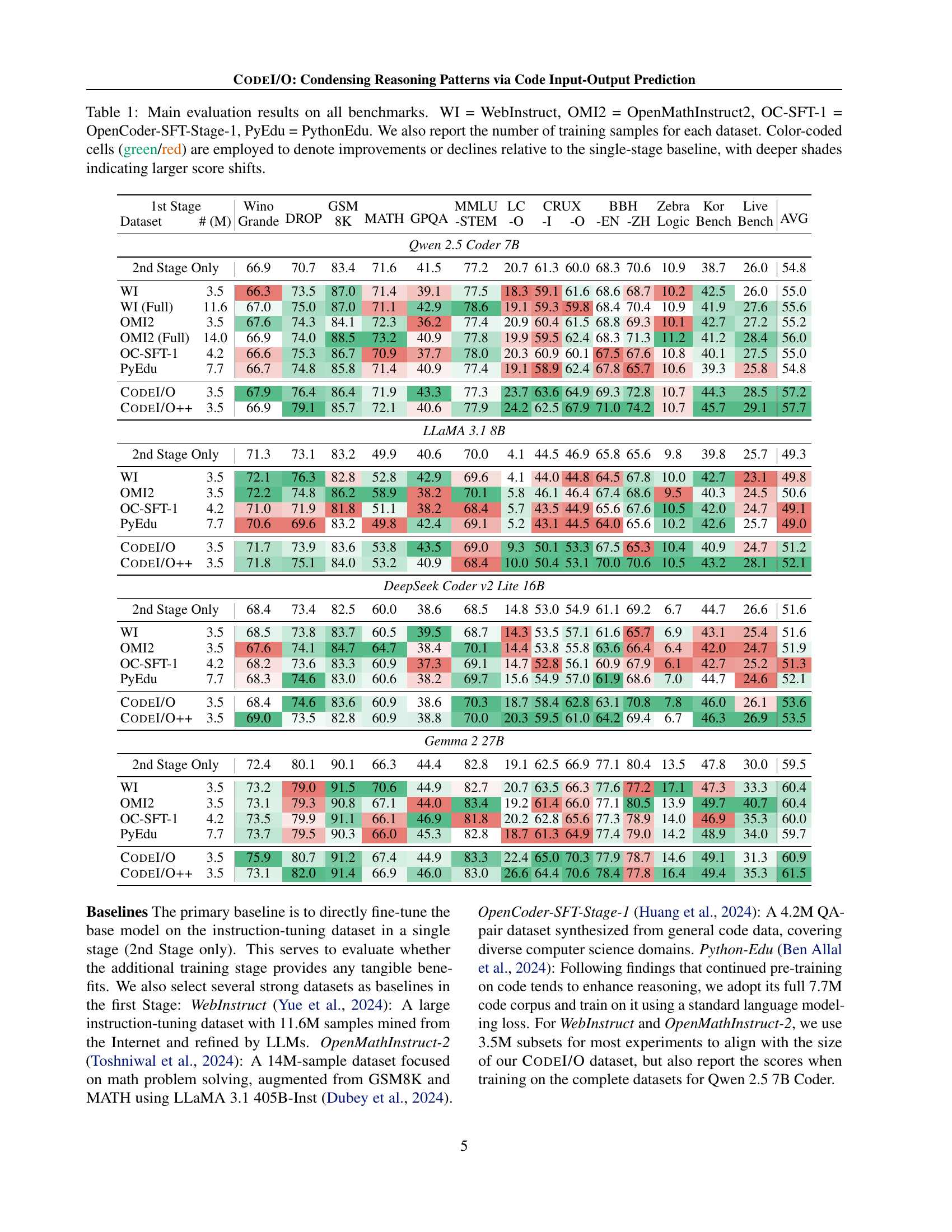
🔼 Table 1 presents the main experimental results across fourteen benchmark datasets, evaluating the performance of four different language models (LLMs). Each model was tested under two training conditions: a single-stage training phase using only instruction-tuning data and a two-stage approach that adds pre-training on either the CODEI/O or CODEI/O++ dataset before instruction tuning. The table shows the performance of each model on each benchmark under both training strategies. Color coding highlights performance improvements (green) or declines (red) compared to the single-stage baseline, with color intensity reflecting the magnitude of the change. The number of training samples for each dataset is also included. The table allows for a direct comparison of different LLMs’ performance across various reasoning tasks, illustrating the impact of the proposed CODEI/O and CODEI/O++ datasets on enhancing reasoning capabilities.
read the caption
Table 1: Main evaluation results on all benchmarks. WI = WebInstruct, OMI2 = OpenMathInstruct2, OC-SFT-1 = OpenCoder-SFT-Stage-1, PyEdu = PythonEdu. We also report the number of training samples for each dataset. Color-coded cells (green/red) are employed to denote improvements or declines relative to the single-stage baseline, with deeper shades indicating larger score shifts.
In-depth insights#
Reasoning in LLMs#
Reasoning in large language models (LLMs) is a rapidly evolving field. Early LLMs primarily focused on pattern matching and statistical prediction, lacking genuine reasoning capabilities. Current research emphasizes improving reasoning abilities, often through techniques like chain-of-thought prompting, which guides the model through a step-by-step reasoning process. However, data sparsity remains a significant challenge; while abundant data exists for tasks like code generation and translation, data for nuanced reasoning tasks is limited. This necessitates innovative approaches to data creation and augmentation, such as the CODEI/O method leveraging reasoning patterns inherent in code. Successfully integrating reasoning abilities into LLMs is crucial for achieving artificial general intelligence (AGI). Evaluating reasoning performance in LLMs is also a complex problem; existing benchmarks may not capture the full spectrum of reasoning abilities, necessitating the development of more comprehensive and robust evaluation metrics. Future research should focus on creating more generalizable and robust reasoning methods and addressing the limitations of current datasets and evaluation techniques.
CODEI/O Approach#
The CODEI/O approach tackles the challenge of sparse and fragmented training data in diverse reasoning tasks by leveraging the rich reasoning patterns inherent in code. Instead of directly training on raw code, it cleverly transforms code into an input/output prediction format. This allows models to learn fundamental reasoning principles (logic flow, state-space search, etc.) decoupled from code-specific syntax. The use of Chain-of-Thought (CoT) rationales expressed in natural language further enhances learning by making the reasoning process explicit. By predicting inputs or outputs given code and test cases, CODEI/O exposes the model to universal reasoning primitives. The approach also incorporates a verification and refinement process (CODEI/O++), which enhances the quality of CoTs through multi-turn revision, leading to improved overall performance. This method offers a scalable and effective way to condense diverse reasoning patterns from readily available code, overcoming limitations of traditional approaches that rely on scarce or fragmented data.
Empirical Findings#
An ‘Empirical Findings’ section in a research paper would present the results of experiments or data analysis conducted to test the hypotheses or address the research questions. A strong section would start with a clear and concise overview of the key findings, perhaps highlighting statistically significant results or unexpected patterns. It would then delve into a detailed presentation of the data, potentially using tables, graphs, and visualizations to aid comprehension. Crucially, the section should not simply report the results but also interpret them within the context of the research questions and existing literature. Comparisons to baselines or control groups are vital, along with a discussion of any limitations or potential biases in the data or methodology. Statistical significance should be explicitly addressed and clearly explained, avoiding jargon. Finally, the empirical findings should be directly linked back to the paper’s overall conclusions and contributions. The writing style should be precise, objective, and easily understandable by the intended audience. A well-written ‘Empirical Findings’ section forms the backbone of a convincing and impactful research paper.
Ablation Studies#
Ablation studies systematically remove components of a model or process to understand their individual contributions. In the context of a research paper, an ablation study on a method like CODEI/O would involve removing or altering specific parts of its design—perhaps removing the input generator, modifying the training data, or changing the prediction format—to assess the impact on overall performance. The results from these experiments help isolate and quantify the effectiveness of each component. For example, removing the multi-turn revision step (CODEI/O++) might show a significant performance drop, highlighting its value in improving reasoning abilities. Similarly, testing with different subsets of training data allows assessment of the model’s robustness and whether certain data sources or reasoning patterns are more crucial than others. Overall, well-designed ablation studies offer strong evidence regarding a model’s strengths, weaknesses, and critical components while providing valuable insights for future improvement. The analysis should thoroughly discuss how each removed or modified component affects performance across different reasoning tasks, leading to a better understanding of the model’s functionality and potential limitations.
Future Work#
Future work in this research area could explore several promising avenues. Improving the efficiency and scalability of the CODEI/O training process is crucial for handling even larger codebases. Investigating alternative data augmentation techniques to further enhance model generalization is essential. Exploring different model architectures beyond the ones tested, potentially incorporating more advanced techniques such as transformers, could lead to better performance. A key area for future work is analyzing the impact of diverse programming languages beyond Python to make CODEI/O more widely applicable. Finally, a thorough investigation into the interplay between CODEI/O and other reasoning methods like chain-of-thought prompting and reinforcement learning could unlock new levels of performance. Addressing these aspects will solidify CODEI/O’s position as a leading approach for enhancing reasoning capabilities in LLMs.
More visual insights#
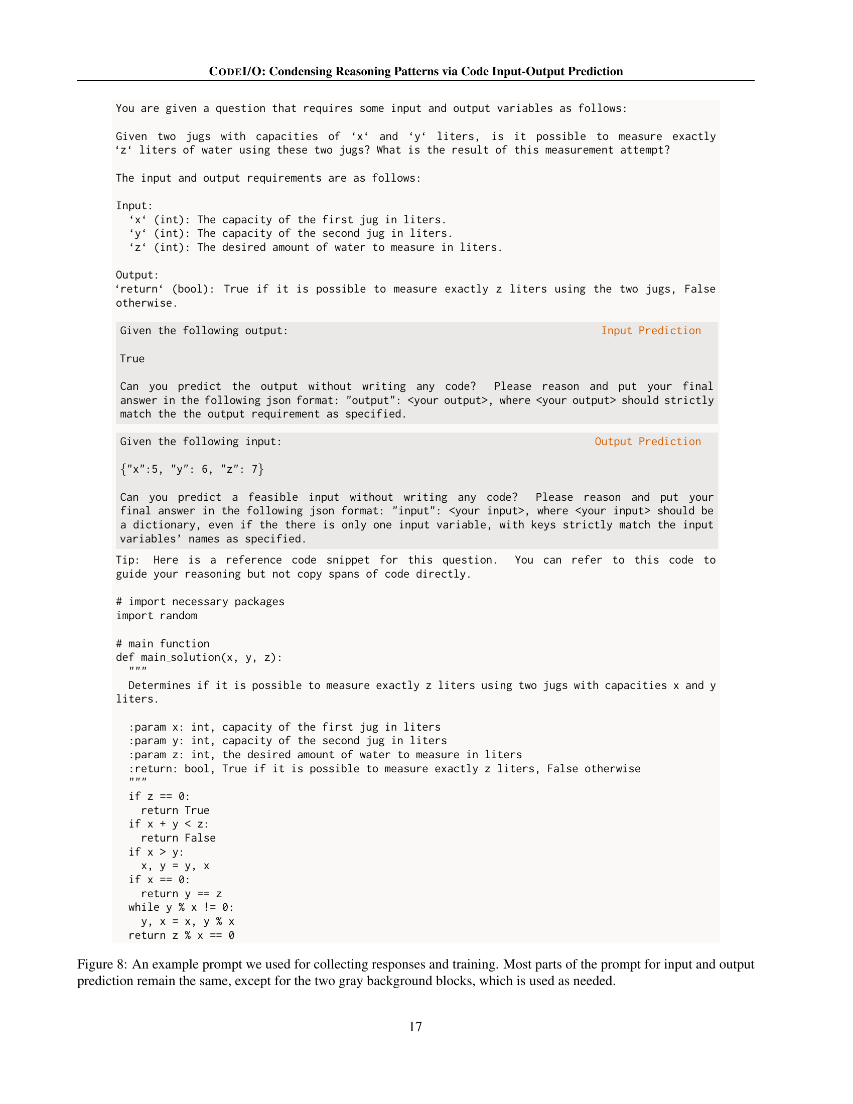
More on figures

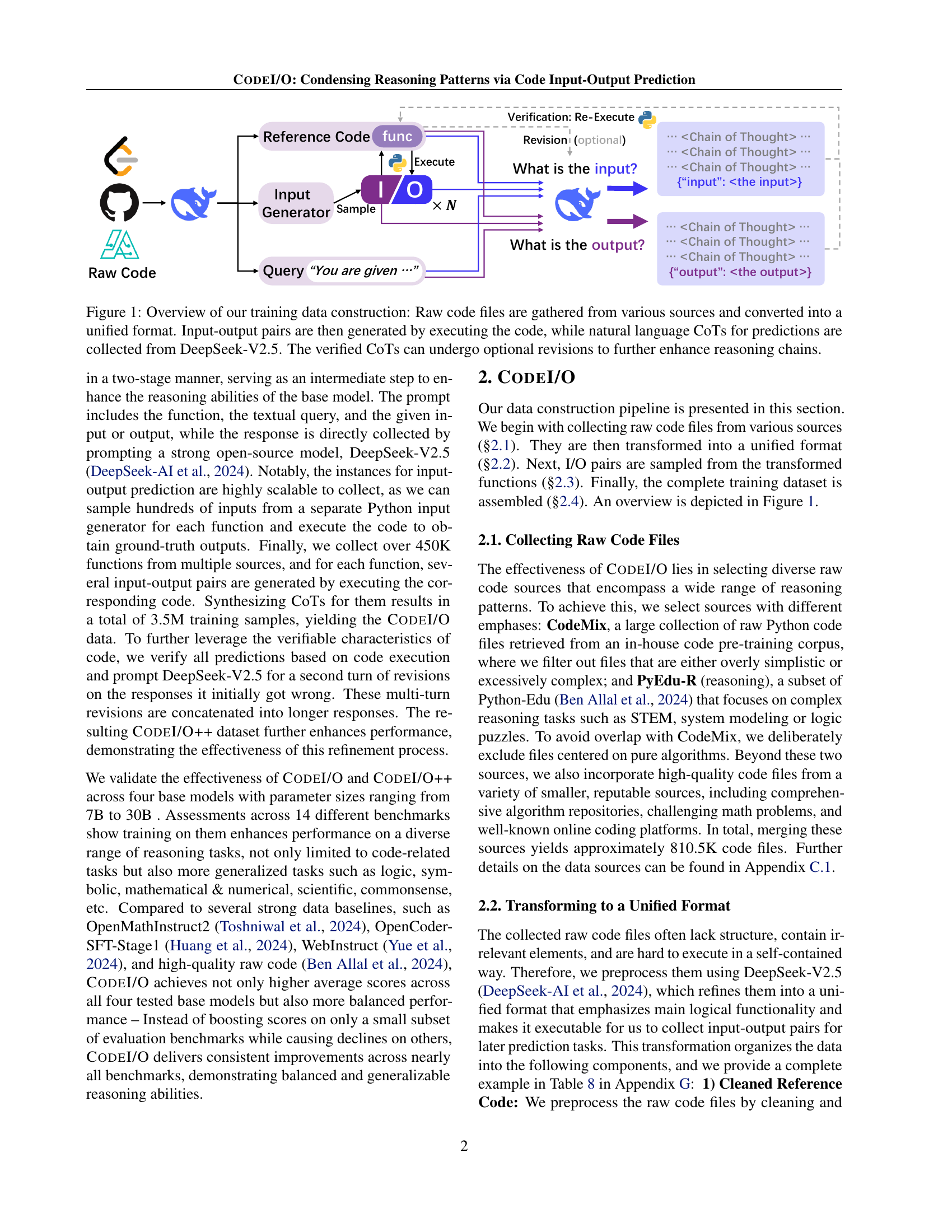
🔼 This figure displays two examples from the CODEI/O dataset illustrating the model’s input and output prediction capabilities. The left example shows a prediction for the output given a specified input. A detailed chain of thought (CoT) is presented, demonstrating how the model arrives at its answer. The right example demonstrates the opposite: predicting the input that would result in a given output. Again, a CoT is shown, outlining the reasoning process. These examples showcase the model’s ability to reason using natural language CoTs, given the code and a query.
read the caption
Figure 2: Two examples for the collected responses for input and output prediction respectively.

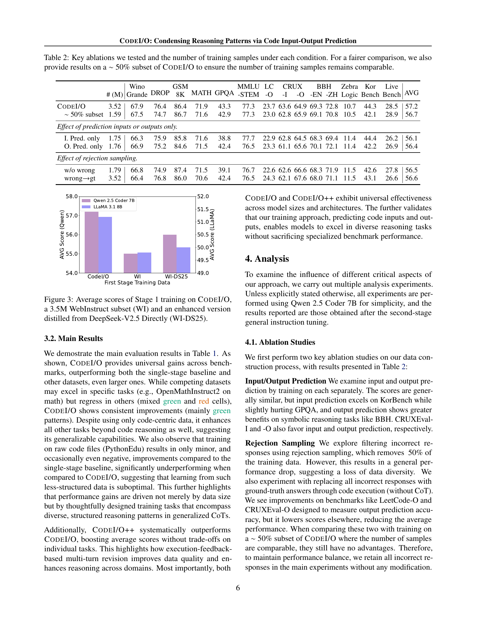
🔼 This figure compares the performance of training a language model on three different datasets in the first stage of a two-stage training process. The three datasets are: 1) CODEI/O, a new dataset created by the authors; 2) WI, a 3.5 million sample subset of the WebInstruct dataset, representing a strong existing instruction tuning dataset; and 3) WI-DS25, an enhanced version of the WebInstruct dataset created by directly distilling knowledge from the DeepSeek-V2.5 model. The figure shows the average scores achieved on various downstream benchmarks after training on these datasets. This allows the reader to compare the effectiveness of the newly proposed CODEI/O dataset against strong existing baselines, showing its improved performance on diverse reasoning tasks.
read the caption
Figure 3: Average scores of Stage 1 training on CodeI/O, a 3.5M WebInstruct subset (WI) and an enhanced version distilled from DeepSeek-V2.5 Directly (WI-DS25).
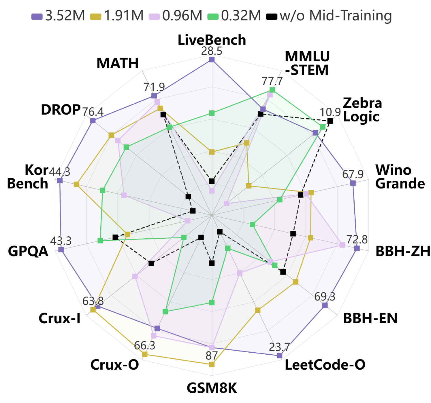
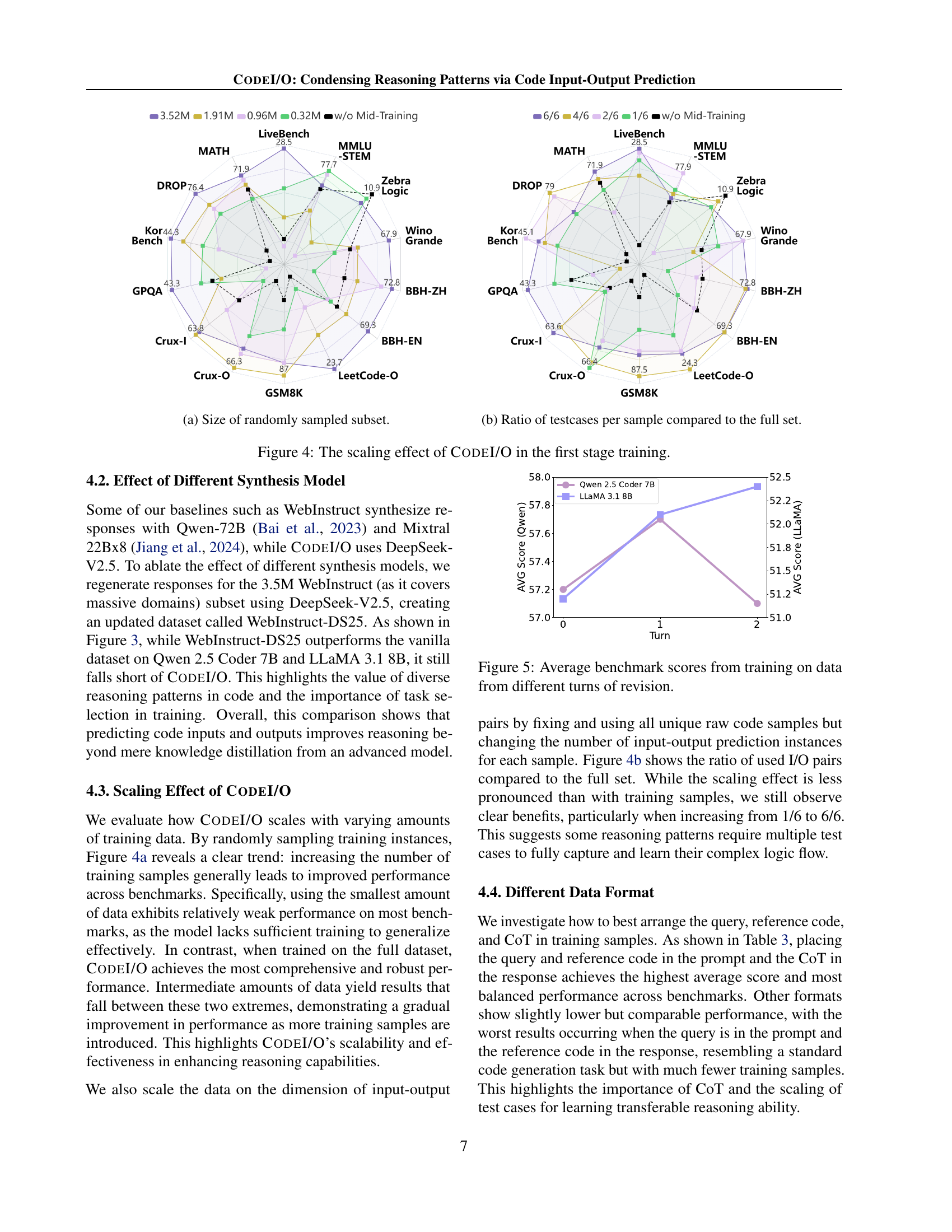
🔼 This figure shows how the model’s performance changes as the size of the training dataset varies. The x-axis represents the size of a randomly selected subset of the CODEI/O training data, ranging from a small fraction of the full dataset to the complete dataset. The y-axis represents the average performance across multiple reasoning benchmarks. The plot illustrates the relationship between training data size and model performance, demonstrating the scaling behavior of the model.
read the caption
(a) Size of randomly sampled subset.

🔼 This figure shows how the model’s performance changes when varying the number of input/output test cases per training sample, while keeping the total number of training samples constant. The x-axis represents the ratio of testcases used compared to the full dataset, showing the scaling effect of the CODEI/O dataset.
read the caption
(b) Ratio of testcases per sample compared to the full set.

🔼 This figure demonstrates the impact of the size and quantity of training data derived from CodeI/O on model performance. The plots show that increasing the size of the training dataset (Panel a) and the number of input/output examples per training sample (Panel b) leads to consistent improvements across various reasoning benchmarks. Larger datasets and more input/output pairs result in better model generalization and higher performance. The results highlight the effectiveness and scalability of the CodeI/O training approach.
read the caption
Figure 4: The scaling effect of CodeI/O in the first stage training.

🔼 This figure displays the average benchmark scores achieved by training language models on data from different revision turns. The x-axis represents the revision turn (0, 1, or 2), indicating whether the model’s responses were used directly (Turn 0), corrected once (Turn 1), or corrected twice (Turn 2). The y-axis shows the average score across multiple benchmark tasks. The different colored lines likely represent different language models or model sizes, allowing for comparison of performance changes across different models when training on progressively revised data. The purpose is to illustrate the impact of iterative response refinement on model performance.
read the caption
Figure 5: Average benchmark scores from training on data from different turns of revision.

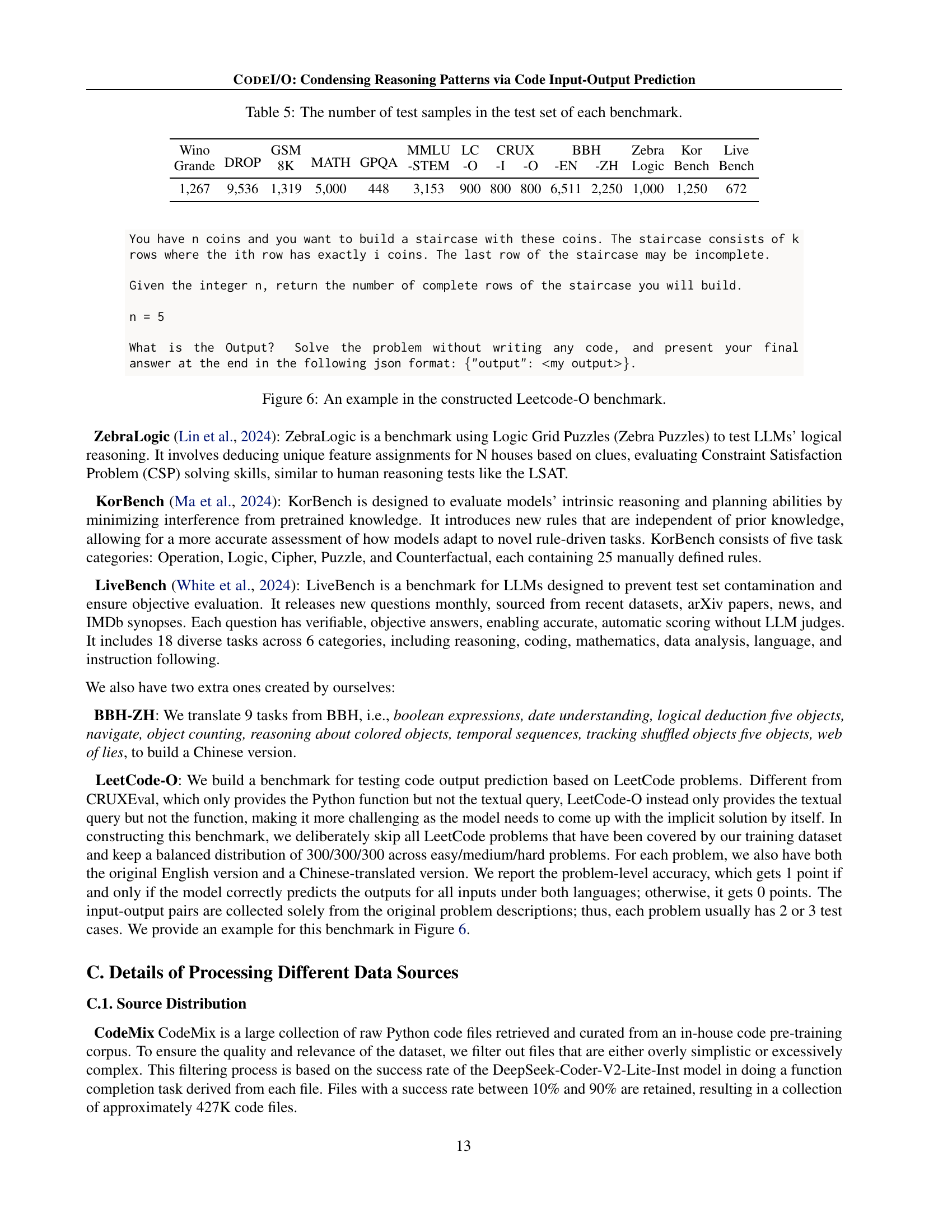
🔼 The figure shows an example problem from the LeetCode-O benchmark dataset. This dataset is specifically designed to test the model’s ability to predict the output of a code given a textual description of the problem, without providing the actual code itself. The example demonstrates a common type of coding problem requiring logical reasoning and algorithmic thinking. The user is given a problem involving coins and asked to determine the number of complete rows in a staircase built using those coins, with the instructions to provide the final answer in a specific JSON format. This illustrates the style and complexity of problems in the LeetCode-O benchmark.
read the caption
Figure 6: An example in the constructed Leetcode-O benchmark.
More on tables
| Wino | DROP | GSM | MATH | GPQA | MMLU | LC | CRUX | BBH | Zebra | Kor | Live | AVG | ||||
| # (M) | Grande | 8K | -STEM | -O | -I | -O | -EN | -ZH | Logic | Bench | Bench | |||||
| CodeI/O | 3.52 | 67.9 | 76.4 | 86.4 | 71.9 | 43.3 | 77.3 | 23.7 | 63.6 | 64.9 | 69.3 | 72.8 | 10.7 | 44.3 | 28.5 | 57.2 |
| 50% subset | 1.59 | 67.5 | 74.7 | 86.7 | 71.6 | 42.9 | 77.3 | 23.0 | 62.8 | 65.9 | 69.1 | 70.8 | 10.5 | 42.1 | 28.9 | 56.7 |
| Effect of prediction inputs or outputs only. | ||||||||||||||||
| I. Pred. only | 1.75 | 66.3 | 75.9 | 85.8 | 71.6 | 38.8 | 77.7 | 22.9 | 62.8 | 64.5 | 68.3 | 69.4 | 11.4 | 44.4 | 26.2 | 56.1 |
| O. Pred. only | 1.76 | 66.9 | 75.2 | 84.6 | 71.5 | 42.4 | 76.5 | 23.3 | 61.1 | 65.6 | 70.1 | 72.1 | 11.4 | 42.2 | 26.9 | 56.4 |
| Effect of rejection sampling. | ||||||||||||||||
| w/o wrong | 1.79 | 66.8 | 74.9 | 87.4 | 71.5 | 39.1 | 76.7 | 22.6 | 62.6 | 66.6 | 68.3 | 71.9 | 11.5 | 42.6 | 27.8 | 56.5 |
| wronggt | 3.52 | 66.4 | 76.8 | 86.0 | 70.6 | 42.4 | 76.5 | 24.3 | 62.1 | 67.6 | 68.0 | 71.1 | 11.5 | 43.1 | 26.6 | 56.6 |
🔼 This table presents ablation studies on the CODEI/O dataset, investigating the impact of various factors on model performance. It compares the full CODEI/O dataset with a 50% subset for a fair comparison, given the varying sizes of other datasets used in the experiment. Ablations include removing data from specific sources (CodeMix and PyEdu-R), using only input or output predictions, and employing rejection sampling (removing incorrect predictions). The results across multiple benchmarks (WinoGrande, DROP, GSM8K, MATH, GPQA, MMLU-STEM, LC-O, CRUX-Eval, BBH, ZebraLogic, KorBench, LiveBench) reveal the contribution of different data aspects to overall model performance.
read the caption
Table 2: Key ablations we tested and the number of training samples under each condition. For a fairer comparison, we also provide results on a ∼similar-to\sim∼ 50% subset of CodeI/O to ensure the number of training samples remains comparable.
| Data Format | Wino | DROP | GSM | MATH | GPQA | MMLU | LC | CRUX | BBH | Zebra | Kor | Live | AVG | |||
|---|---|---|---|---|---|---|---|---|---|---|---|---|---|---|---|---|
| Prompt | Response | Grande | 8K | -STEM | -O | -I | -O | -EN | -ZH | Logic | Bench | Bench | ||||
| Q+Code | CoT | 67.9 | 76.4 | 86.4 | 71.9 | 43.3 | 77.3 | 23.7 | 63.6 | 64.9 | 69.3 | 72.8 | 10.7 | 44.3 | 28.5 | 57.2 |
| Q | CoT | 67.2 | 76.8 | 87.2 | 70.4 | 37.5 | 77.3 | 25.2 | 62.6 | 65.3 | 69.2 | 71.1 | 11.5 | 44.9 | 28.5 | 56.8 |
| Code | CoT | 67.9 | 76.4 | 87.0 | 70.8 | 39.5 | 76.5 | 25.0 | 64.1 | 65.8 | 68.8 | 71.3 | 10.6 | 45.2 | 28.5 | 57.0 |
| Q | Code+CoT | 65.9 | 76.1 | 87.5 | 71.7 | 42.2 | 76.9 | 22.9 | 63.9 | 66.1 | 69.6 | 72.9 | 10.9 | 41.4 | 28.5 | 56.9 |
| Q | Code | 66.9 | 73.1 | 84.8 | 71.6 | 40.0 | 77.4 | 20.8 | 59.5 | 62.4 | 67.2 | 68.3 | 10.1 | 40.3 | 26.3 | 54.9 |
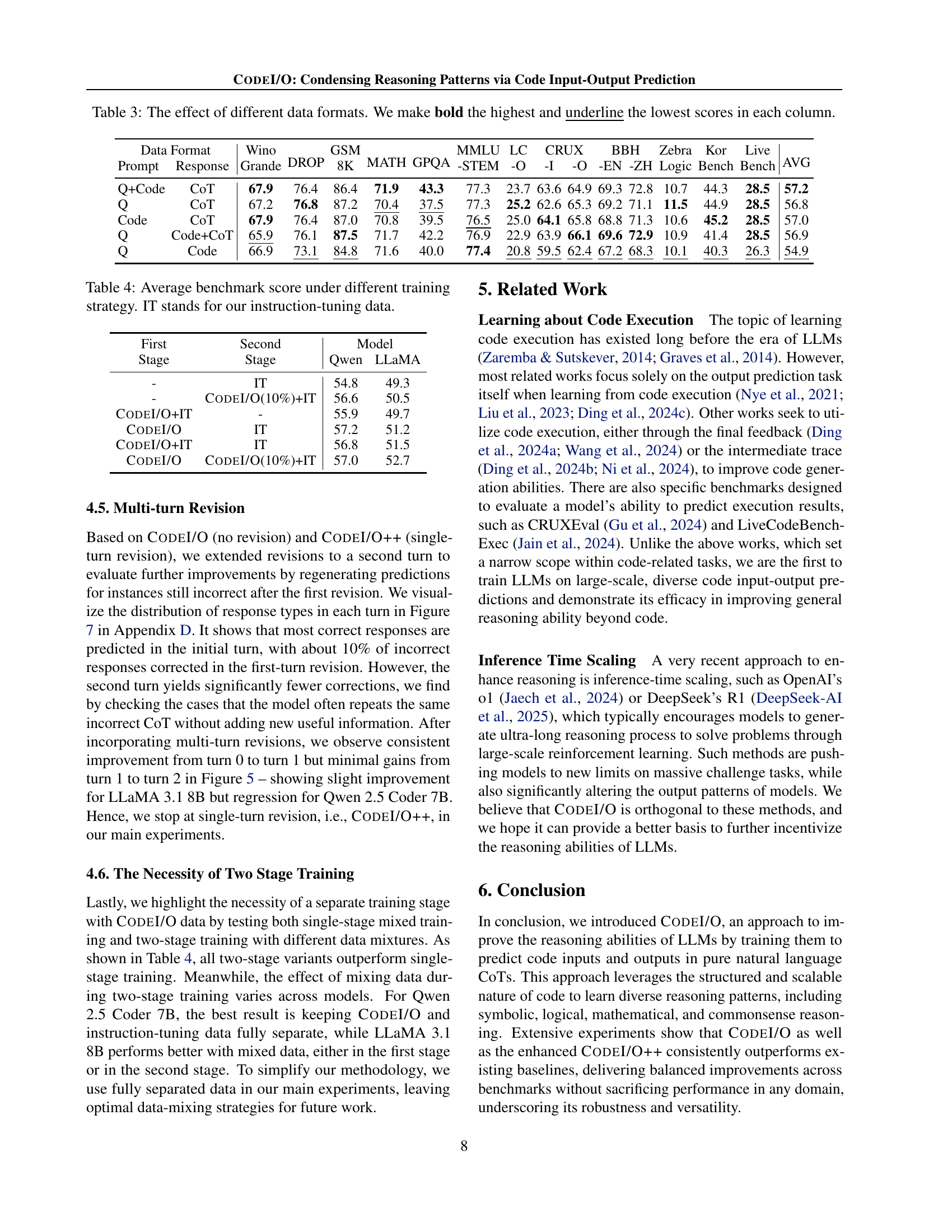
🔼 This table presents the results of an ablation study on different data formats used in training. The study explores how different arrangements of query, code, and chain-of-thought (CoT) affect model performance. The table shows the average scores across various benchmarks for different arrangements of this information in training samples. Each row represents a different format, and columns show benchmark scores (higher scores are better). The highest score in each column is bolded, and the lowest score is underlined, highlighting the optimal data format.
read the caption
Table 3: The effect of different data formats. We make bold the highest and underline the lowest scores in each column.
| First | Second | Model | |
|---|---|---|---|
| Stage | Stage | Qwen | LLaMA |
| - | IT | 54.8 | 49.3 |
| - | CodeI/O(10%)+IT | 56.6 | 50.5 |
| CodeI/O+IT | - | 55.9 | 49.7 |
| CodeI/O | IT | 57.2 | 51.2 |
| CodeI/O+IT | IT | 56.8 | 51.5 |
| CodeI/O | CodeI/O(10%)+IT | 57.0 | 52.7 |
🔼 This table presents the average benchmark scores achieved by different training strategies. It compares models trained using various combinations of the CODEI/O and CODEI/O++ datasets with and without additional instruction tuning data (IT). This allows for an analysis of how each data source and the training methodology influences the performance across a range of reasoning tasks.
read the caption
Table 4: Average benchmark score under different training strategy. IT stands for our instruction-tuning data.
| Wino | DROP | GSM | MATH | GPQA | MMLU | LC | CRUX | BBH | Zebra | Kor | Live | ||
| Grande | 8K | -STEM | -O | -I | -O | -EN | -ZH | Logic | Bench | Bench | |||
| 1,267 | 9,536 | 1,319 | 5,000 | 448 | 3,153 | 900 | 800 | 800 | 6,511 | 2,250 | 1,000 | 1,250 | 672 |
🔼 This table presents the number of test samples used for evaluating the performance of different reasoning models on a set of benchmark datasets. It provides a quantitative overview of the scale of each benchmark and helps to understand the relative size and scope of the evaluation tasks. The benchmarks encompass diverse reasoning domains such as commonsense reasoning, numerical reasoning, logical deduction, and code understanding. The number of samples varies across benchmarks, indicating differences in the difficulty and complexity of the tasks.
read the caption
Table 5: The number of test samples in the test set of each benchmark.
| Wino | DROP | GSM | MATH | GPQA | MMLU | LC | CRUX | BBH | Zebra | Kor | Live | AVG | ||||
|---|---|---|---|---|---|---|---|---|---|---|---|---|---|---|---|---|
| # (M) | Grande | 8K | -STEM | -O | -I | -O | -EN | -ZH | Logic | Bench | Bench | |||||
| CodeI/O | 3.52 | 67.9 | 76.4 | 86.4 | 71.9 | 43.3 | 77.3 | 23.7 | 63.6 | 64.9 | 69.3 | 72.8 | 10.7 | 44.3 | 28.5 | 57.2 |
| 50% subset | 1.59 | 67.5 | 74.7 | 86.7 | 71.6 | 42.9 | 77.3 | 23.0 | 62.8 | 65.9 | 69.1 | 70.8 | 10.5 | 42.1 | 28.9 | 56.7 |
| w/o CodeMix | 1.84 | 65.8 | 76.6 | 87.3 | 70.9 | 42.6 | 77.0 | 21.8 | 62.0 | 65.0 | 68.5 | 69.5 | 10.7 | 43.8 | 26.8 | 56.3 |
| w/o PyEdu-R | 1.89 | 66.8 | 75.4 | 86.0 | 71.4 | 40.6 | 77.0 | 24.1 | 61.8 | 64.8 | 69.8 | 72.3 | 11.0 | 46.3 | 30.1 | 57.0 |
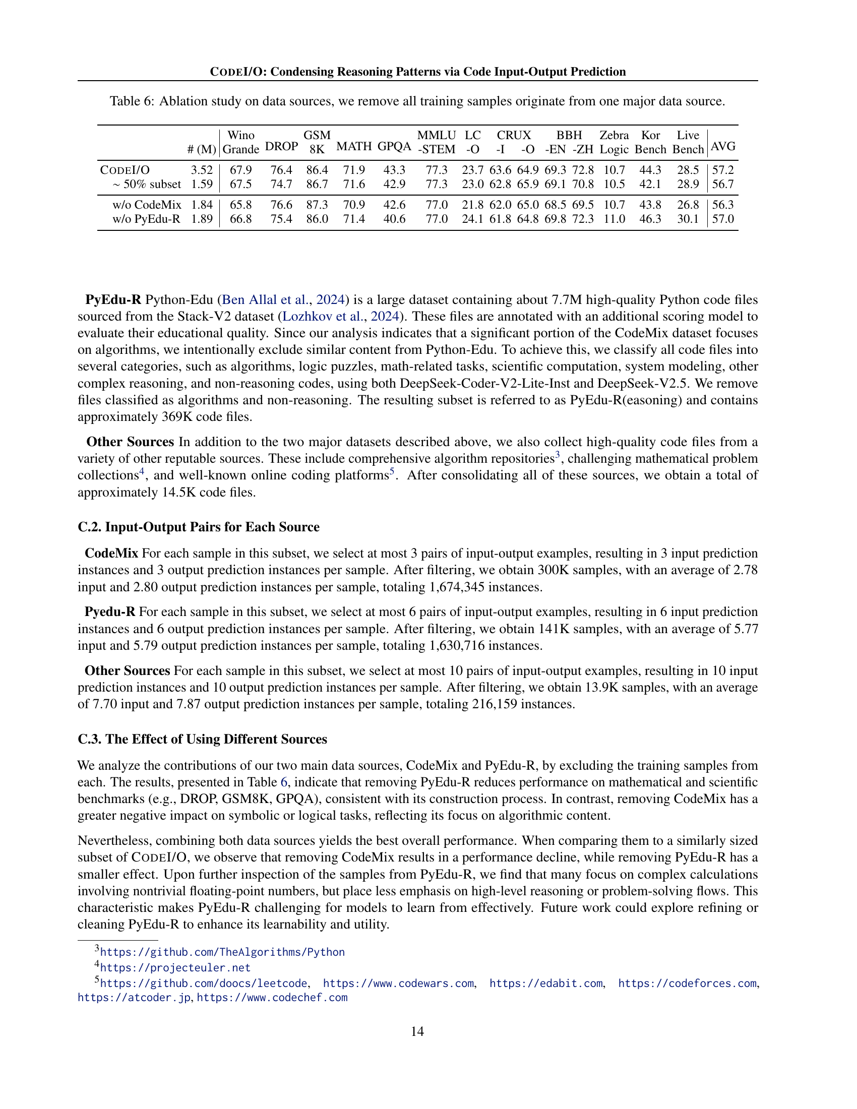
🔼 This table presents an ablation study analyzing the impact of removing one major data source from the CODEI/O training dataset. It shows the performance across various reasoning benchmarks when training data from either CodeMix or PyEdu-R is excluded. The results highlight the relative contributions of each data source to overall model performance on different reasoning tasks, indicating which source is more crucial for specific types of reasoning.
read the caption
Table 6: Ablation study on data sources, we remove all training samples originate from one major data source.
| Wino | DROP | GSM | MATH | GPQA | MMLU | LC | CRUX | BBH | Zebra | Kor | Live | AVG | ||||
|---|---|---|---|---|---|---|---|---|---|---|---|---|---|---|---|---|
| Stage 1 | Stage 2 | Grande | 8K | -STEM | -O | -I | -O | -EN | -ZH | Logic | Bench | Bench | ||||
| - | Tulu3 | 66.9 | 59.9 | 81.0 | 38.3 | 27.2 | 69.3 | 16.6 | 53.9 | 59.9 | 63.9 | 69.8 | 8.9 | 35.2 | 22.5 | 48.1 |
| CodeI/O | Tulu3 | 68.1 | 59.4 | 79.3 | 39.8 | 30.4 | 71.3 | 17.6 | 57.1 | 64.3 | 65.8 | 72.5 | 8.6 | 43.4 | 22.4 | 50.0 |
| CodeI/O++ | Tulu3 | 67.6 | 54.9 | 80.5 | 39.9 | 27.5 | 71.9 | 20.6 | 57.3 | 63.3 | 66.6 | 70.0 | 9.3 | 41.8 | 24.3 | 49.7 |
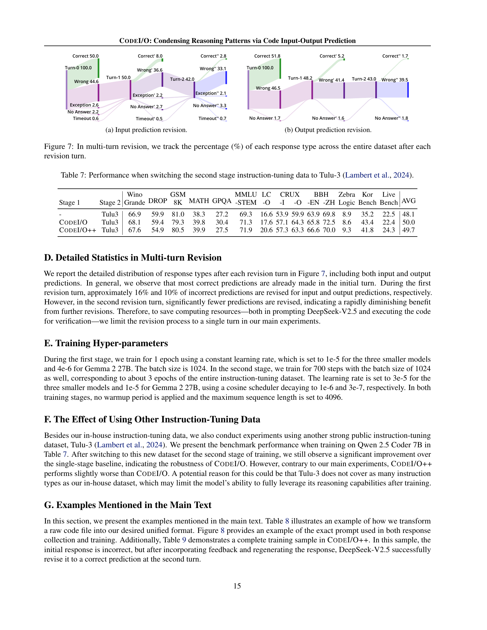
🔼 This table presents the results of an experiment comparing the performance of language models trained with two different instruction tuning datasets. The experiment uses four different base language models (Qwen 2.5 Coder 7B, LLaMA 3.1 8B, DeepSeek Coder v2 Lite 16B, and Gemma 2 27B). Each model was trained in two stages. The first stage uses the CODEI/O or CODEI/O++ dataset, while the second stage employs either the original instruction-tuning dataset or the Tulu-3 dataset (Lambert et al., 2024) as a replacement. The table shows the performance of these models across multiple reasoning benchmarks, highlighting the impact of switching the instruction-tuning dataset in the second stage of training.
read the caption
Table 7: Performance when switching the second stage instruction-tuning data to Tulu-3 (Lambert et al., 2024).
| Raw Code File | Cleaned Reference Code (with Main Entrypoint Function) |
|---|---|
| ⬇ #get the vertical acceleration data acceleration [. . . . . . . . ] # pass acceleration data to low pass filter time[. . . . . . . . . . . . ] #code to find speed at each point initial_speed = current_speed delta_t = t_current - t_prev curr_acc = acc[i] current_speed = initial_speed + (curr_acc) * delta_t #code to find dispacement initial_dis = current_disp delta_t = t_current - t_prev curr_speed = ("call above algorithm") current_disp = initial_dis + (initial_speed + current_speed)/2 * delta_t ; #code to find horizontal displacement #use the above same code and find horizontal displacement #pass both the displacement data through low pass filter #map horizontal and vertical displacement to give road profile | ⬇ # import necessary packages import numpy as np # main function def main_solution(acceleration, time, initial_speed, initial_displacement): # Convert inputs to numpy arrays if they are not already acceleration = np.array(acceleration) time = np.array(time) # Initialize variables current_speed = initial_speed current_disp = initial_displacement # Calculate speed and displacement speeds = [] displacements = [] for i in range(1, len(time)): delta_t = time[i] - time[i-1] curr_acc = acceleration[i] current_speed = current_speed + curr_acc * delta_t speeds.append(current_speed) current_disp = current_disp + (initial_speed + current_speed) / 2 * delta_t displacements.append(current_disp) initial_speed = current_speed # Convert outputs to JSON serializable format speeds = [float(speed) for speed in speeds] displacements = [float(disp) for disp in displacements] return {"speeds": speeds, "displacements": displacements} |
| Query | |
| Given a set of vertical acceleration data and corresponding time points, how can we determine the speed and displacement of a vehicle at each time point, starting from an initial speed and displacement? | |
| Input/Output Description | Input Generator |
| ⬇ Input: acceleration (list of float): List of vertical acceleration values at each time point. time (list of float): List of time points corresponding to the acceleration values. initial_speed (float): Initial speed at the first time point. initial_displacement (float): Initial displacement at the first time point. Output: return (dict): A dictionary with two keys: - speeds (list of float): List of calculated speeds at each time point. - displacements (list of float): List of calculated displacements at each time point. | ⬇ def input_generator(): # Generate random acceleration data acceleration = [np.random.uniform(-10, 10) for _ in range(10)] # Generate corresponding time data time = [0.1 * i for i in range(10)] # Generate initial speed and displacement initial_speed = np.random.uniform(0, 10) initial_displacement = np.random.uniform(0, 10) return { "acceleration": acceleration, "time": time, "initial_speed": initial_speed, "initial_displacement": initial_displacement } |
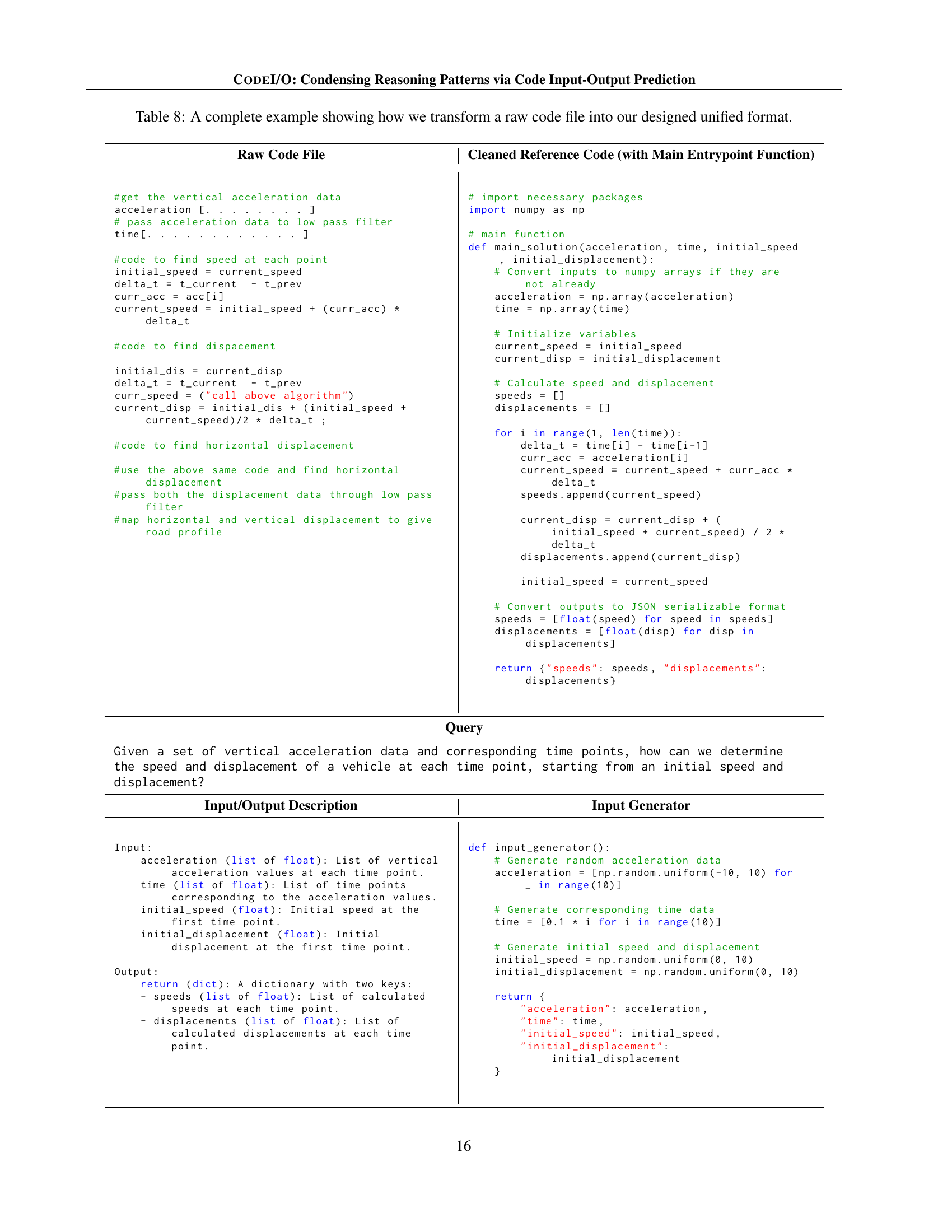
🔼 This table showcases a complete example of how the authors transform raw code from a real-world project into the structured format they use for their CODEI/O dataset. It demonstrates the process of cleaning, restructuring, generating input/output pairs, and preparing prompts and outputs for training a language model. It highlights each step involved in creating the final, unified format used for the model training, covering aspects like code cleaning, defining main functions, creating input generators, and crafting comprehensive queries.
read the caption
Table 8: A complete example showing how we transform a raw code file into our designed unified format.
| Prompt |
|---|
| You are given a question that requires some input and output variables as follows: Given a list of integers numbers and an integer target, determine the length of the shortest contiguous subarray whose sum is at least target. If no such subarray exists, return 0. How can you find this shortest subarray length efficiently? The input and output requirements are as follows: Input: - target (int): The target sum that the subarray should at least reach. - numbers (list of int): A list of integers representing the array from which the subarray is to be found. Output: - return (int): The length of the shortest contiguous subarray whose sum is at least the target. Returns 0 if no such subarray exists. Given the following output: 4 Can you predict a feasible input without writing any code? Please reason and put your final answer in the following json format: {"input": your input}, where your input should be a dictionary with keys strictly match the input variables’ names as specified. |
| Concatenated Response (Turn 1 generation + Turn 1 feedback + Turn 2 generation + Turn 2 feedback) |
| To predict a feasible input that results in the output 4, we need to consider the following: 1. Target Sum: The target sum is the minimum sum that a subarray should achieve. 2. Numbers List: The list of integers from which we need to find the shortest subarray. 3. Output: The length of the shortest subarray whose sum is at least the target. Given the output is 4, this means the shortest subarray that meets or exceeds the target sum has a length of 4. ### Reasoning: - Target Sum: Let’s assume the target sum is 10. - Numbers List: We need to construct a list where the shortest subarray that sums to at least 10 has a length of 4. ### Example Construction: - If we have a list like [1, 2, 3, 4, 5], the subarray [2, 3, 4, 5] sums to 14, which is greater than 10, and its length is 4. Thus, a feasible input that results in the output 4 could be: ‘‘‘json
{"input": {"target": 10, "numbers": [1, 2, 3, 4, 5]}}
‘‘‘
This input satisfies the condition that the shortest subarray with a sum of at least 10 has a length of 4.Let me check if I did it correctly …… Oops! Something went wrong and I find this [Mismatch] Your input is not feasible! Given the output 4, your predicted input is {"target": 10, "numbers": [1, 2, 3, 4, 5]}, which actually gets a wrong output as 3 Well …… I apologize for the oversight. Let’s re-evaluate the input to ensure it matches the output 4. We need to find a list of integers where the shortest contiguous subarray whose sum is at least target has a length of exactly 4. ### Revised Reasoning: - Target Sum: Let’s keep the target sum as 10. - Numbers List: We need a list where a subarray of length 4 sums to 10 or more. ### Example Construction: - Consider the list [1, 2, 2, 2, 2, 2]: - The subarray [2, 2, 2, 2] sums to 8, which is less than 10. - However, if we add another 2, making it [1, 2, 2, 2, 2, 2, 2], the subarray [2, 2, 2, 2] still sums to 8. - Let’s try a different approach with larger numbers to ensure the subarray of length 4 sums to at least 10: - Consider the list [1, 3, 2, 2, 5, 1]: - The subarray [1, 3, 2, 2] sums to 8, which is less than 10. - The subarray [3, 2, 2, 5] sums to 12, which is more than 10, and its length is 4. Thus, a feasible input that results in the output 4 could be: ‘‘‘jsonΩ
{"input": {"target": 10, "numbers": [1, 3, 2, 2, 5, 1]}}
‘‘‘
This input satisfies the condition that the shortest subarray with a sum of at least 10 has a length of 4.Let me check if I did it correctly …… Yes, that’s correct! I made it! |
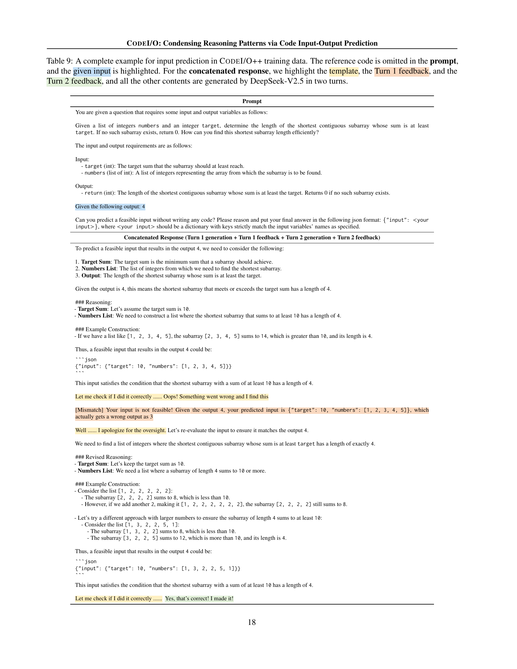
🔼 This table showcases a complete example from the CodeI/O++ dataset used for training input prediction models. The example illustrates the two-stage process of response generation. The initial prompt omits the reference code but highlights the given input. The model’s response is then evaluated, and if incorrect, feedback is provided, prompting the model to generate a revised response. The table displays the original prompt, the model’s first response, the feedback indicating the error, the second response, and final feedback confirming the correction. This demonstrates how iterative feedback refines the model’s reasoning process.
read the caption
Table 9: A complete example for input prediction in CodeI/O++ training data. The reference code is omitted in the prompt, and the given input is highlighted. For the concatenated response, we highlight the template, the Turn 1 feedback, and the Turn 2 feedback, and all the other contents are generated by DeepSeek-V2.5 in two turns.
Full paper#