TL;DR#
Autoregressive models have become the standard for video generation, but they suffer from slow inference speeds due to their sequential, token-by-token generation process. This approach often struggles to capture spatial dependencies effectively within video frames. Prior work has attempted to resolve this by using methods like multi-token prediction, but these methods either introduce additional modules or impose significant constraints, thus hindering their effectiveness and scalability.
This paper introduces a novel semi-autoregressive framework called Next-Block Prediction (NBP) that addresses these limitations. Instead of predicting individual tokens, NBP predicts entire blocks of tokens simultaneously. This parallelization significantly reduces the number of generation steps, leading to faster inference. NBP also employs bidirectional attention within each block to better capture spatial dependencies. Experiments demonstrate that NBP significantly outperforms existing methods in terms of both speed and generation quality, achieving speed-ups exceeding 11 times on standard benchmarks.
Key Takeaways#
Why does it matter?#
This paper is crucial because it presents a novel approach to video generation, significantly improving efficiency and scalability compared to existing methods. Its semi-autoregressive framework and next-block prediction strategy offer a new avenue for research in video generation, potentially impacting applications like video editing, special effects, and AI-driven content creation. The results demonstrate substantial speed improvements, paving the way for more efficient and powerful video generation models. Moreover, the scalability of the method makes it adaptable to various model sizes, offering flexibility for researchers with different computational resources. This advancement is particularly important in the context of increasing demand for high-quality, computationally efficient video generation.
Visual Insights#

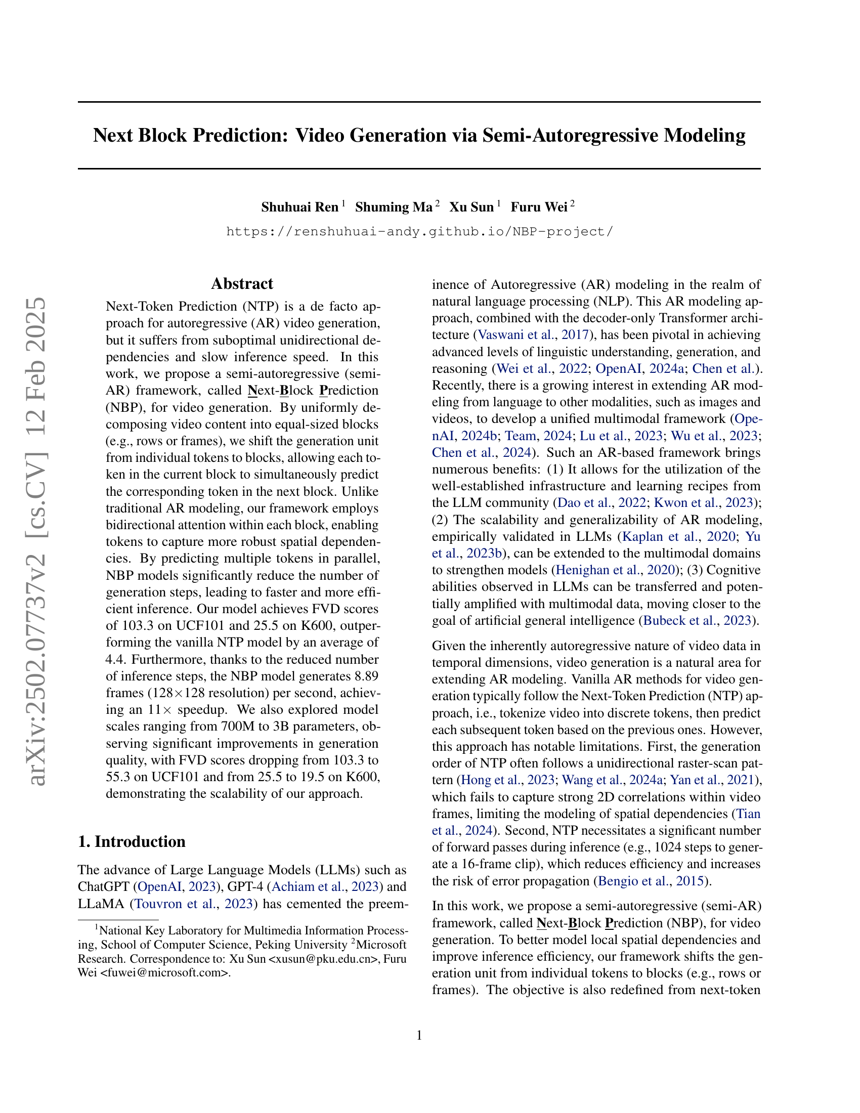
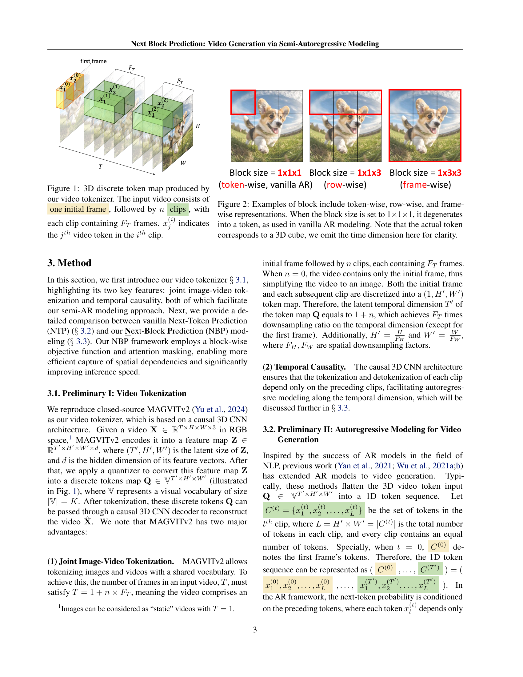
🔼 This figure illustrates the 3D discrete token map generated by the video tokenizer used in the paper. The input video is processed as a sequence. It begins with a single initial frame, followed by a series of clips, each containing a fixed number of frames (FT). Each element in the 3D map, represented as xj(i), signifies a specific video token. The indices (i) and (j) denote the clip number and the token’s position within that clip respectively.
read the caption
Figure 1: 3D discrete token map produced by our video tokenizer. The input video consists of one initial frame, followed by n𝑛nitalic_n clips, with each clip containing FTsubscript𝐹𝑇F_{T}italic_F start_POSTSUBSCRIPT italic_T end_POSTSUBSCRIPT frames. xj(i)subscriptsuperscript𝑥𝑖𝑗x^{(i)}_{j}italic_x start_POSTSUPERSCRIPT ( italic_i ) end_POSTSUPERSCRIPT start_POSTSUBSCRIPT italic_j end_POSTSUBSCRIPT indicates the jthsuperscript𝑗𝑡ℎj^{th}italic_j start_POSTSUPERSCRIPT italic_t italic_h end_POSTSUPERSCRIPT video token in the ithsuperscript𝑖𝑡ℎi^{th}italic_i start_POSTSUPERSCRIPT italic_t italic_h end_POSTSUPERSCRIPT clip.
| Block Size | Block Shape (THW) | FVD |
|---|---|---|
| 16 | 144 | 33.4 |
| 16 | 218 | 29.2 |
| 16 | 1116 | 25.5 |
| 8 | 222 | 32.7 |
| 8 | 118 | 25.7 |
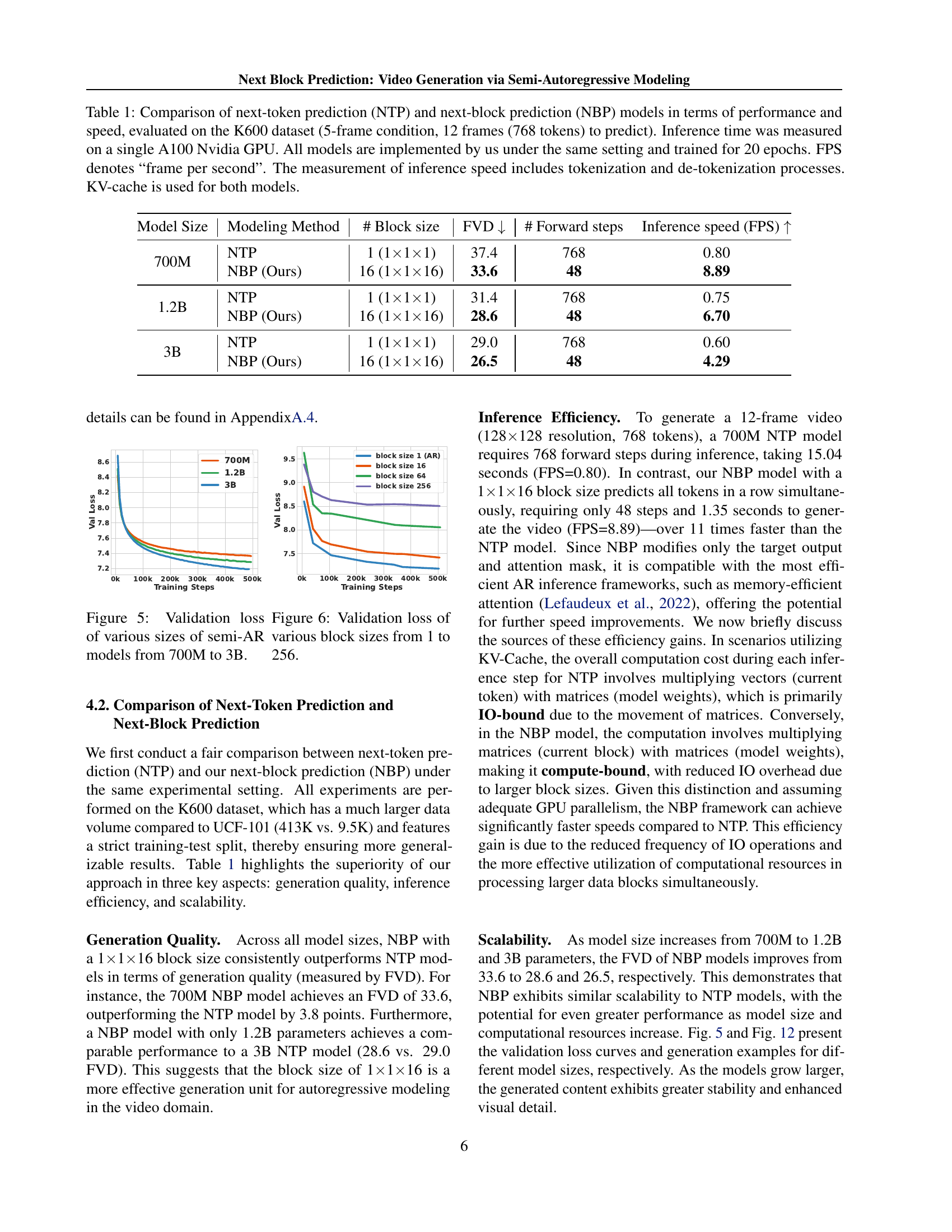
🔼 This table compares the performance and speed of Next-Token Prediction (NTP) and Next-Block Prediction (NBP) models for video generation. The comparison is based on the Kinetics-600 dataset, using a 5-frame condition and predicting 12 frames (768 tokens). Key metrics include Fréchet Video Distance (FVD) to assess video quality, the number of forward steps required during inference, and frames per second (FPS) to measure inference speed. All models were implemented and trained under identical conditions (20 epochs on a single NVIDIA A100 GPU). The inference speed includes the time taken for both tokenization and de-tokenization processes. The KV-cache was used for both model types.
read the caption
Table 1: Comparison of next-token prediction (NTP) and next-block prediction (NBP) models in terms of performance and speed, evaluated on the K600 dataset (5-frame condition, 12 frames (768 tokens) to predict). Inference time was measured on a single A100 Nvidia GPU. All models are implemented by us under the same setting and trained for 20 epochs. FPS denotes “frame per second”. The measurement of inference speed includes tokenization and de-tokenization processes. KV-cache is used for both models.
In-depth insights#
Semi-AR VideoGen#
Semi-autoregressive (Semi-AR) video generation methods offer a compelling alternative to traditional autoregressive approaches. By processing video data in blocks instead of individual tokens, Semi-AR VideoGen significantly accelerates inference speed while maintaining, and potentially improving, generation quality. The approach leverages parallel processing capabilities, reducing the computational burden of generating sequences frame-by-frame. This is crucial for high-resolution videos and complex scenes where the number of tokens to predict is substantial. Moreover, the use of bidirectional attention within each block allows for a more robust capture of spatial dependencies compared to unidirectional models. This results in improved contextual understanding and coherence in the generated video content. However, challenges remain in optimizing block size and configuration, as well as exploring different block structures and shapes to best suit the temporal dynamics of diverse video sequences. Further research should focus on optimizing these hyperparameters and evaluating performance across a wider range of video datasets and generation tasks. Balancing computational efficiency with the quality of the generated video remains a key challenge for future developments in this area.
Block Prediction#
The concept of ‘Block Prediction’ in video generation presents a compelling alternative to traditional next-token prediction methods. By processing video data in blocks (e.g., sequences of frames or rows of pixels), instead of individual tokens, it offers significant advantages in computational efficiency and inference speed. This approach allows for parallel prediction of multiple tokens, leading to a substantial reduction in the number of prediction steps required for video generation. Furthermore, bidirectional attention mechanisms within each block enable more robust modeling of spatial dependencies, which is a notable improvement over unidirectional approaches that may hinder contextual understanding. Although this method relies on a uniform block decomposition of video, which might not be suitable for all videos, the trade-off between efficiency and potential loss of subtle details is worth investigating further for different video types and applications. The effectiveness of ‘Block Prediction’ hinges on the appropriate selection of block size and shape, influencing both speed and model performance. This suggests that careful parameter tuning is crucial to fully harness the potential of this method.
Efficiency Gains#
The efficiency gains in semi-autoregressive video generation, as explored in the research paper, stem primarily from a paradigm shift: moving from predicting individual tokens (next-token prediction or NTP) to predicting blocks of tokens (next-block prediction or NBP) simultaneously. This parallelization drastically reduces the number of inference steps, leading to a significant speedup. The paper highlights an 11x speed increase with minimal performance degradation, achieving comparable FVD scores to NTP models with substantially fewer steps. Bidirectional attention within each block further contributes to efficiency gains by allowing tokens to better capture spatial dependencies, improving model robustness and reducing computation. The framework’s scalability, demonstrated through experiments across varying model sizes (700M to 3B parameters), suggests that these efficiency benefits are not confined to smaller models, but are consistent across different model scales. The uniform decomposition of video content into equal-sized blocks allows for efficient processing and effective parallelization, offering significant advantages for high-resolution videos and computationally intensive tasks.
Scalability Tests#
In assessing the scalability of a video generation model, a robust testing strategy is crucial. Comprehensive scalability tests should involve systematically increasing model parameters (e.g., 700M, 1.2B, 3B parameters) while carefully monitoring performance metrics such as Fréchet Video Distance (FVD) and frames per second (FPS). A successful scalability test demonstrates consistent improvement in video generation quality (lower FVD) with increasing model size, indicating the model’s ability to effectively leverage additional parameters. Simultaneously, assessing the impact on inference speed (FPS) reveals the trade-off between model size and computational efficiency. Ideally, scalability should manifest as both improved quality and acceptable speed, even at larger scales. Analyzing the validation loss curves during training for different model sizes provides additional insights into model learning dynamics and potential bottlenecks. Careful consideration of hardware limitations is also essential when performing scalability tests, ensuring that experimental results are not skewed by resource constraints. The results of such tests are crucial for determining the optimal model size and deployment strategies.
Future Scope#
The future scope of semi-autoregressive video generation, as explored in the research paper, is vast and exciting. Improving efficiency remains paramount, with opportunities to explore more sophisticated attention mechanisms and more efficient decoding strategies to speed up inference and reduce computational costs. Scaling to higher resolutions and longer video sequences is another crucial direction; current models often struggle with high-resolution video generation, both in terms of speed and quality. Enhanced model architectures could leverage advancements in large language models, incorporating innovative techniques for capturing long-range dependencies and intricate spatio-temporal relationships in video data more effectively. Finally, expanding capabilities beyond simple video generation is also essential; future research could focus on integrating other modalities (text, audio), enabling conditional video generation from multi-modal input, and even exploring interactive video generation where user input influences the output. Addressing ethical considerations surrounding deepfake generation, through techniques like watermarking, is also critical for responsible development.
More visual insights#
More on figures
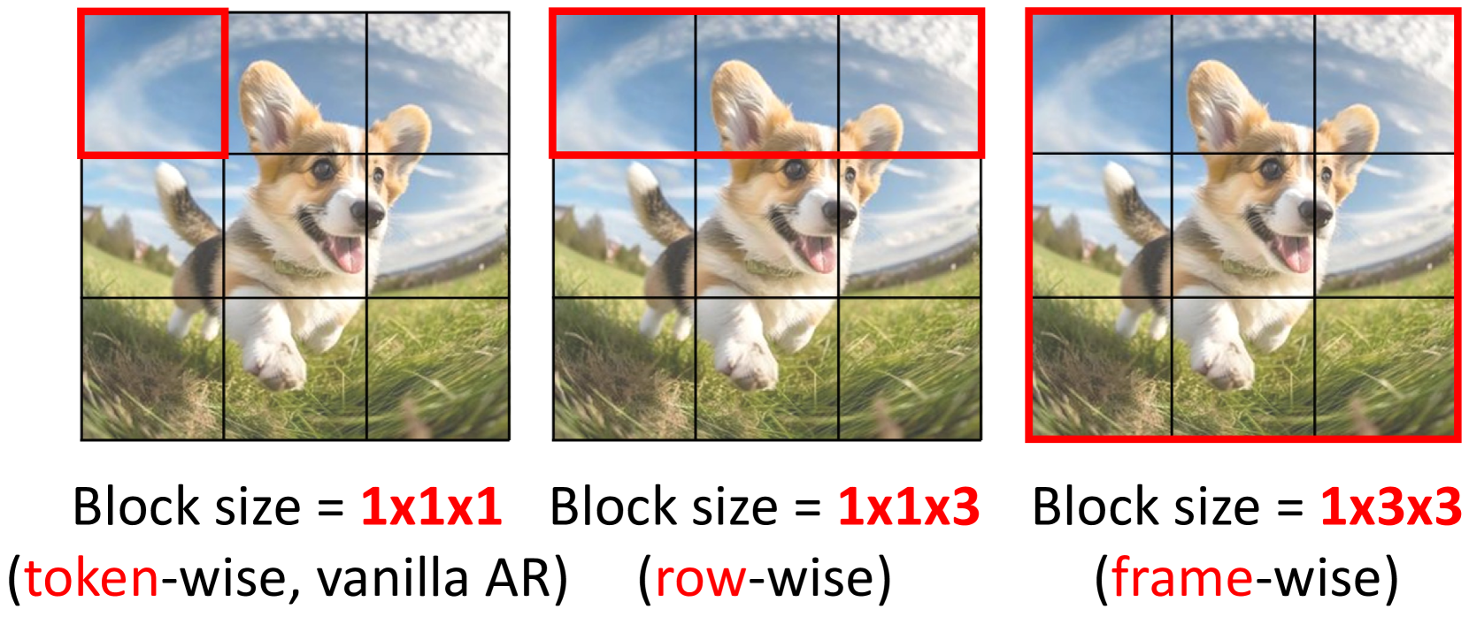
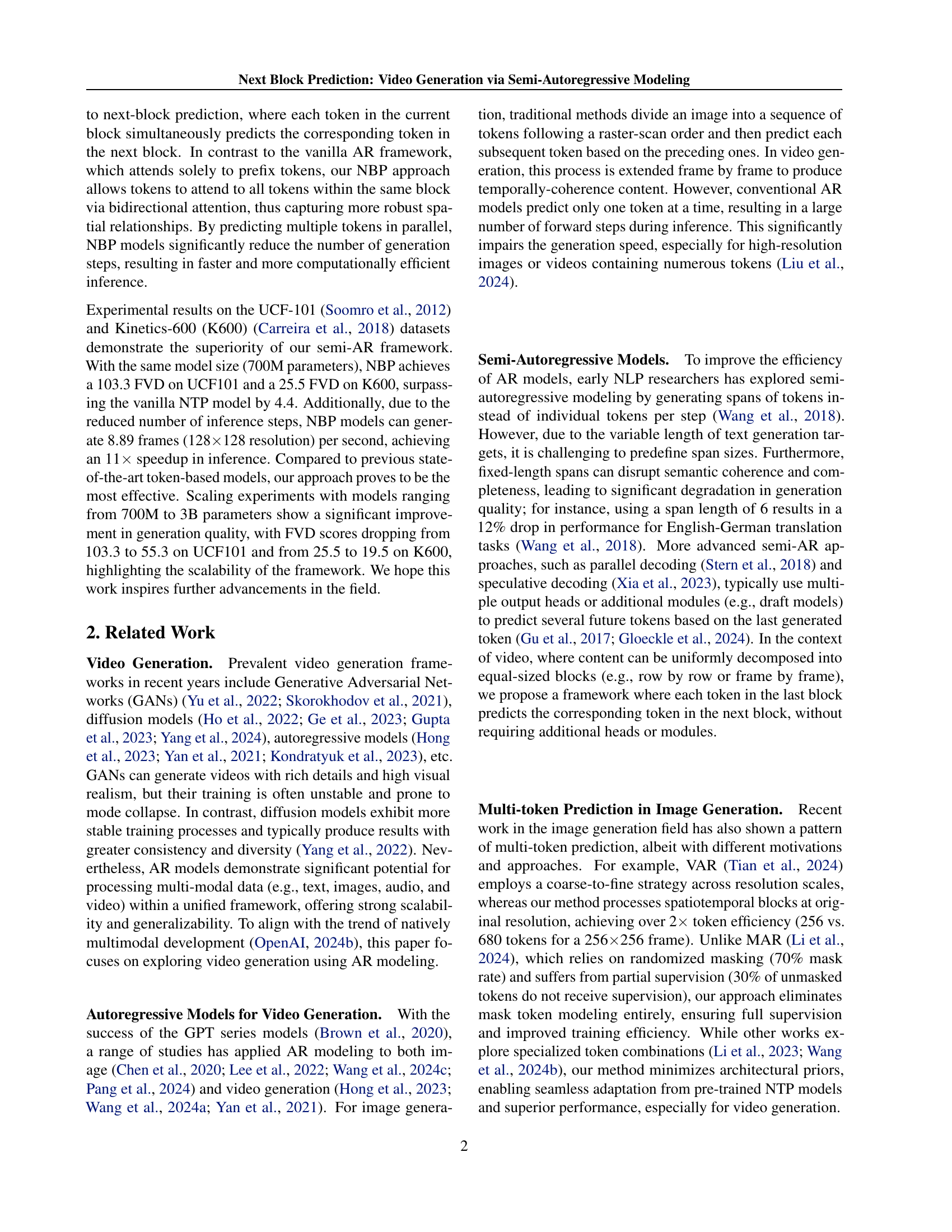
🔼 This figure illustrates different ways to group tokens in a 3D video representation. Standard autoregressive (AR) models process tokens individually (token-wise), treating each pixel or voxel as a separate unit in the generation process. This figure shows alternative block configurations. A row-wise block considers a horizontal line of tokens as a unit, a frame-wise block considers all tokens in one frame as a unit. This allows for parallel processing across multiple tokens in each block instead of generating tokens one by one. When a block size of 1x1x1 is used, it defaults back to the individual token approach of vanilla AR, showing how the block-based approaches generalize the individual token approach.
read the caption
Figure 2: Examples of block include token-wise, row-wise, and frame-wise representations. When the block size is set to 1×\times×1×\times×1, it degenerates into a token, as used in vanilla AR modeling. Note that the actual token corresponds to a 3D cube, we omit the time dimension here for clarity.

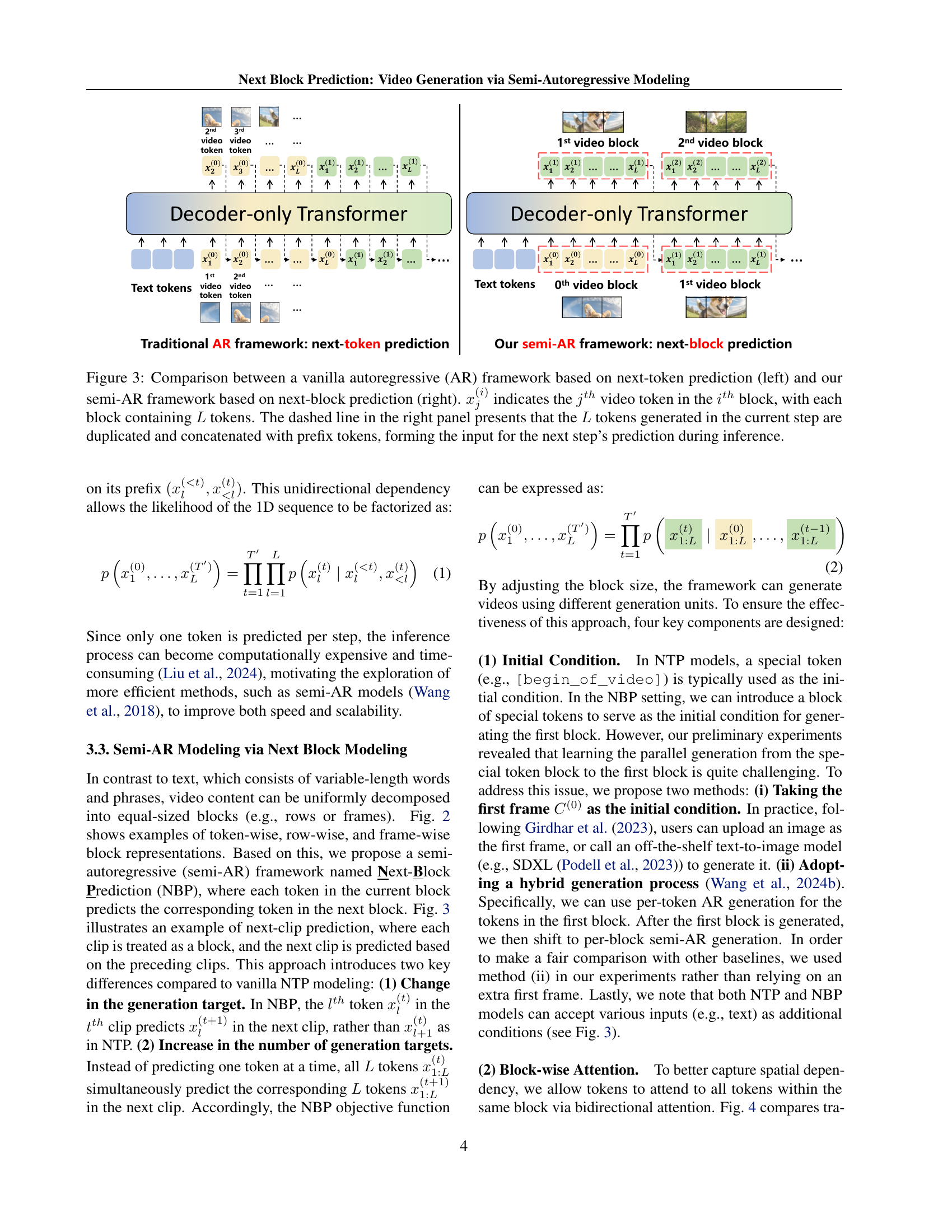
🔼 This figure compares the vanilla autoregressive (AR) model with next-token prediction and the proposed semi-AR model with next-block prediction. The vanilla AR model (left) generates one token at a time, sequentially, using a decoder-only transformer. Each token depends only on the preceding tokens. In contrast, the semi-AR model (right) generates a block of tokens simultaneously. Each token in the current block predicts the corresponding token in the next block, taking advantage of bidirectional attention within the block to capture spatial dependencies. During inference in the semi-AR model, the generated block of tokens is duplicated and concatenated with prefix tokens to form the input for the next prediction step.
read the caption
Figure 3: Comparison between a vanilla autoregressive (AR) framework based on next-token prediction (left) and our semi-AR framework based on next-block prediction (right). xj(i)subscriptsuperscript𝑥𝑖𝑗x^{(i)}_{j}italic_x start_POSTSUPERSCRIPT ( italic_i ) end_POSTSUPERSCRIPT start_POSTSUBSCRIPT italic_j end_POSTSUBSCRIPT indicates the jthsuperscript𝑗𝑡ℎj^{th}italic_j start_POSTSUPERSCRIPT italic_t italic_h end_POSTSUPERSCRIPT video token in the ithsuperscript𝑖𝑡ℎi^{th}italic_i start_POSTSUPERSCRIPT italic_t italic_h end_POSTSUPERSCRIPT block, with each block containing L𝐿Litalic_L tokens. The dashed line in the right panel presents that the L𝐿Litalic_L tokens generated in the current step are duplicated and concatenated with prefix tokens, forming the input for the next step’s prediction during inference.
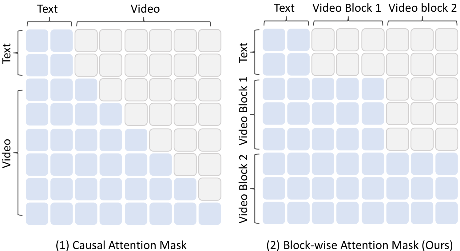
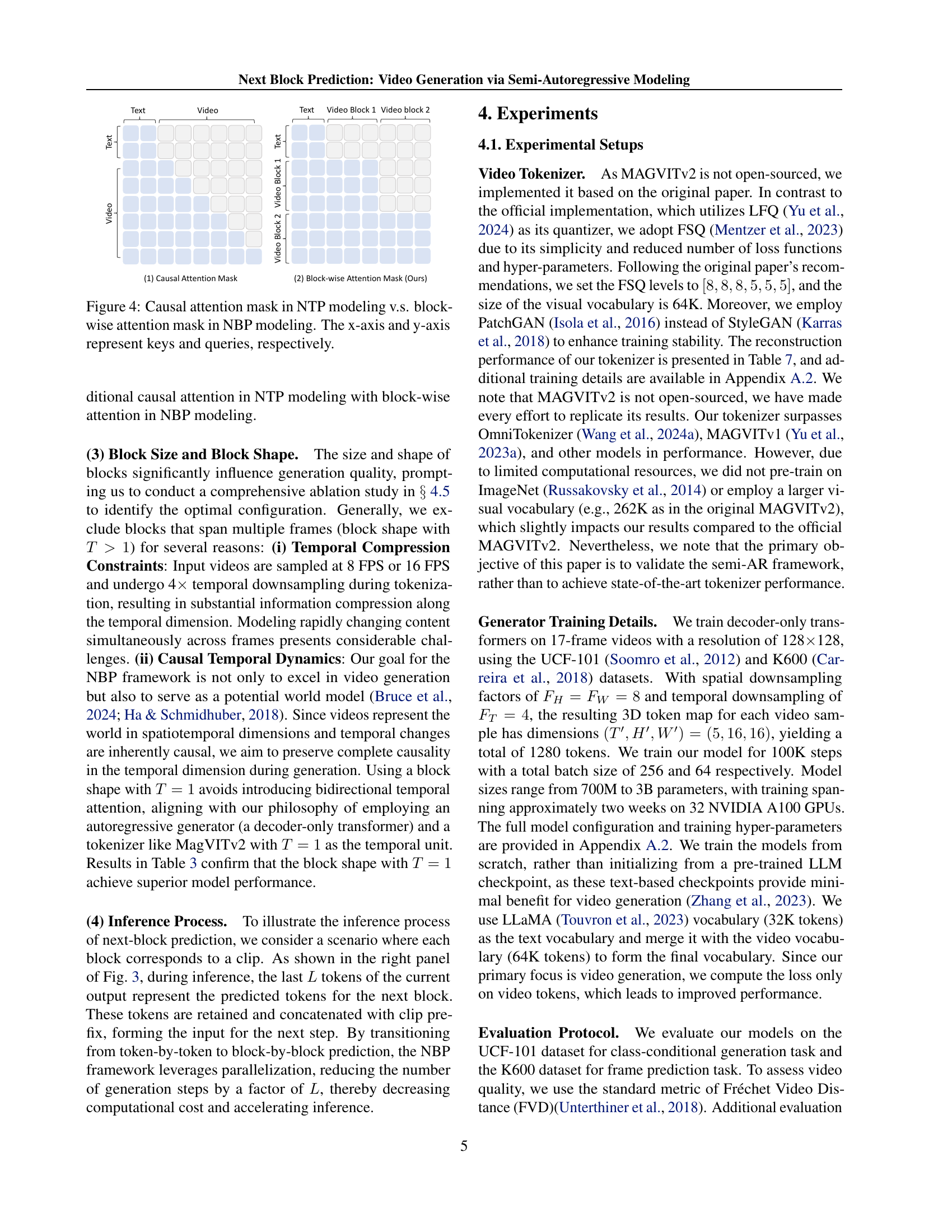
🔼 This figure compares the attention mechanisms used in traditional Next-Token Prediction (NTP) and the proposed Next-Block Prediction (NBP) models. In NTP, the attention is strictly causal, meaning each token only attends to previous tokens, represented by a lower triangular attention mask. This limitation restricts the model’s ability to capture long-range dependencies. In contrast, NBP employs a block-wise attention mechanism. Within each block, tokens can attend to all other tokens in the block bidirectionally, enabling richer contextual understanding. The figure highlights this difference by showing the attention masks for both methods. The x-axis and y-axis represent the keys and queries of the attention mechanism, respectively.
read the caption
Figure 4: Causal attention mask in NTP modeling v.s. block-wise attention mask in NBP modeling. The x-axis and y-axis represent keys and queries, respectively.

🔼 This figure shows the validation loss curves during the training process for semi-autoregressive (semi-AR) video generation models with different parameter scales: 700M, 1.2B, and 3B. The x-axis represents the number of training steps, and the y-axis shows the validation loss. The curves illustrate how the model’s performance changes as it trains, with different sized models exhibiting various learning rates and convergence behaviors. The plot allows for comparison of the training efficiency and stability across models of differing sizes.
read the caption
Figure 5: Validation loss of various sizes of semi-AR models from 700M to 3B.

🔼 This figure shows the validation loss curves for different block sizes used in the Next-Block Prediction (NBP) model during training. The x-axis represents the number of training steps, and the y-axis represents the validation loss. Multiple lines are plotted, each corresponding to a different block size, ranging from 1 to 256. The plot illustrates how the model’s performance changes with varying block sizes during training. The optimal block size that balances training efficiency and model performance can be determined by analyzing this graph.
read the caption
Figure 6: Validation loss of various block sizes from 1 to 256.

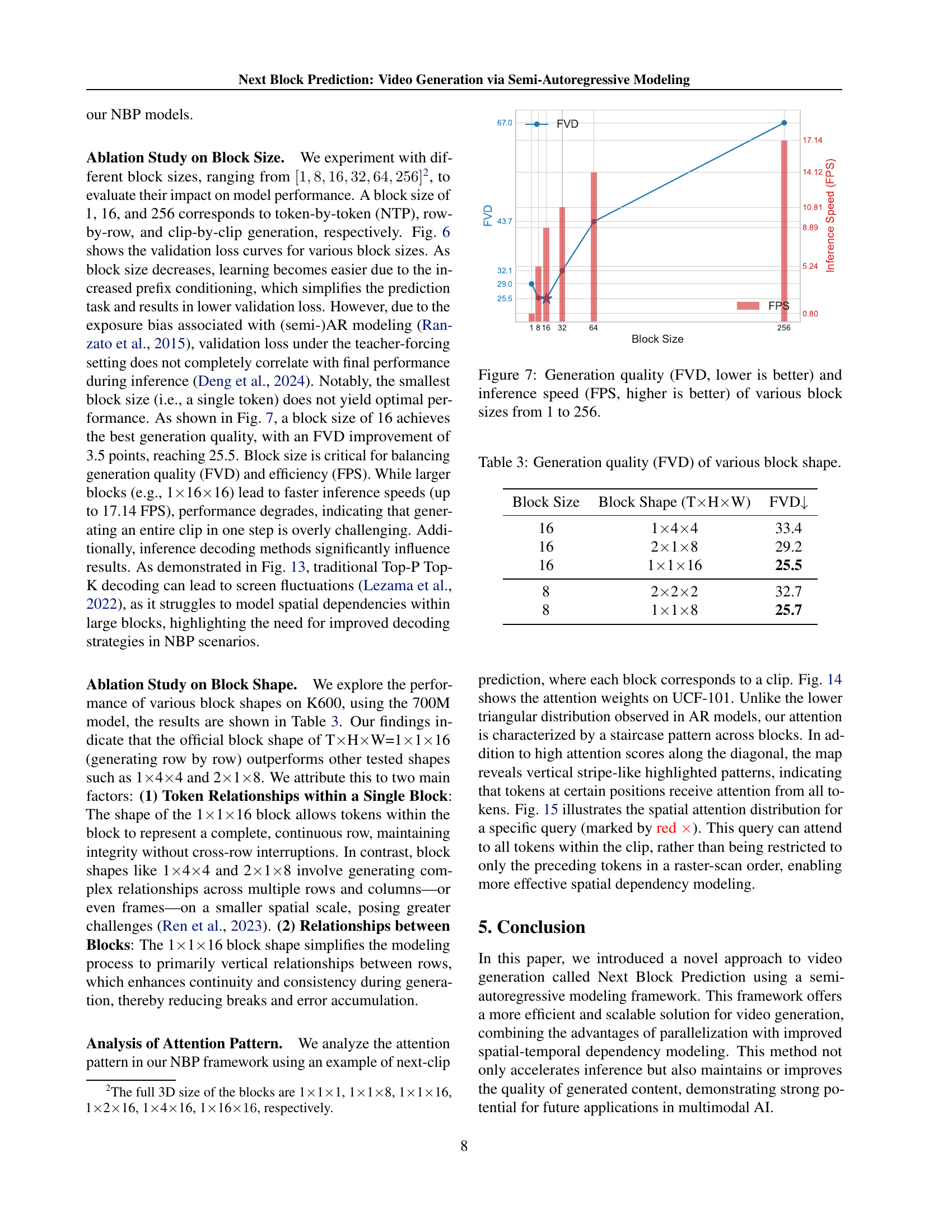
🔼 This figure shows a comparison of the generation quality (measured by Fréchet Video Distance, FVD) and inference speed (frames per second, FPS) of the Next-Block Prediction (NBP) model using different block sizes for video generation. The x-axis represents the block size, ranging from 1 to 256, where a block size of 1 corresponds to the traditional next-token prediction method. The y-axis shows both the FVD score and the FPS. A lower FVD indicates higher generation quality (closer to the ground truth), while a higher FPS indicates faster inference. The graph visually demonstrates the trade-off between generation quality and inference speed as the block size changes, allowing readers to identify an optimal block size that balances both.
read the caption
Figure 7: Generation quality (FVD, lower is better) and inference speed (FPS, higher is better) of various block sizes from 1 to 256.

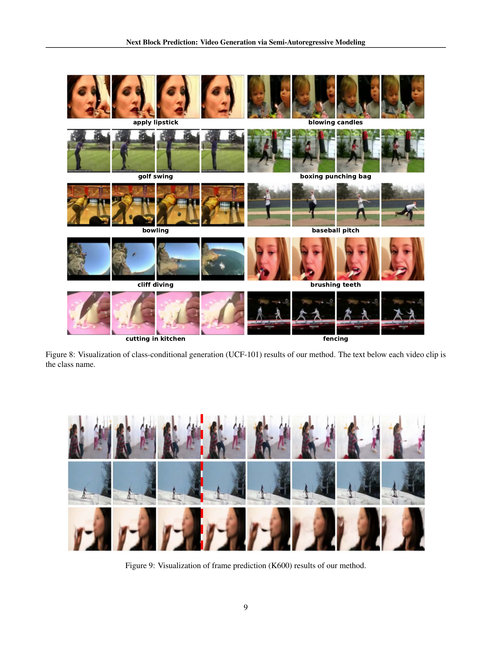
🔼 This figure visualizes the results of class-conditional video generation on the UCF-101 dataset using the proposed Next-Block Prediction (NBP) method. Each row presents a different action class from UCF-101. Multiple video clips generated for each class are displayed, demonstrating the model’s ability to generate diverse instances of each action. The text below each set of video clips indicates the specific action class being depicted.
read the caption
Figure 8: Visualization of class-conditional generation (UCF-101) results of our method. The text below each video clip is the class name.

🔼 This figure shows example results of the model’s frame prediction capabilities on the Kinetics-600 dataset. Each row represents a video sequence where the model has predicted subsequent frames based on a given initial set of frames. The results demonstrate the model’s ability to generate temporally coherent and visually plausible video frames, accurately continuing the action or scene from the input. This showcases the model’s capacity to generate realistic and smooth video sequences.
read the caption
Figure 9: Visualization of frame prediction (K600) results of our method.

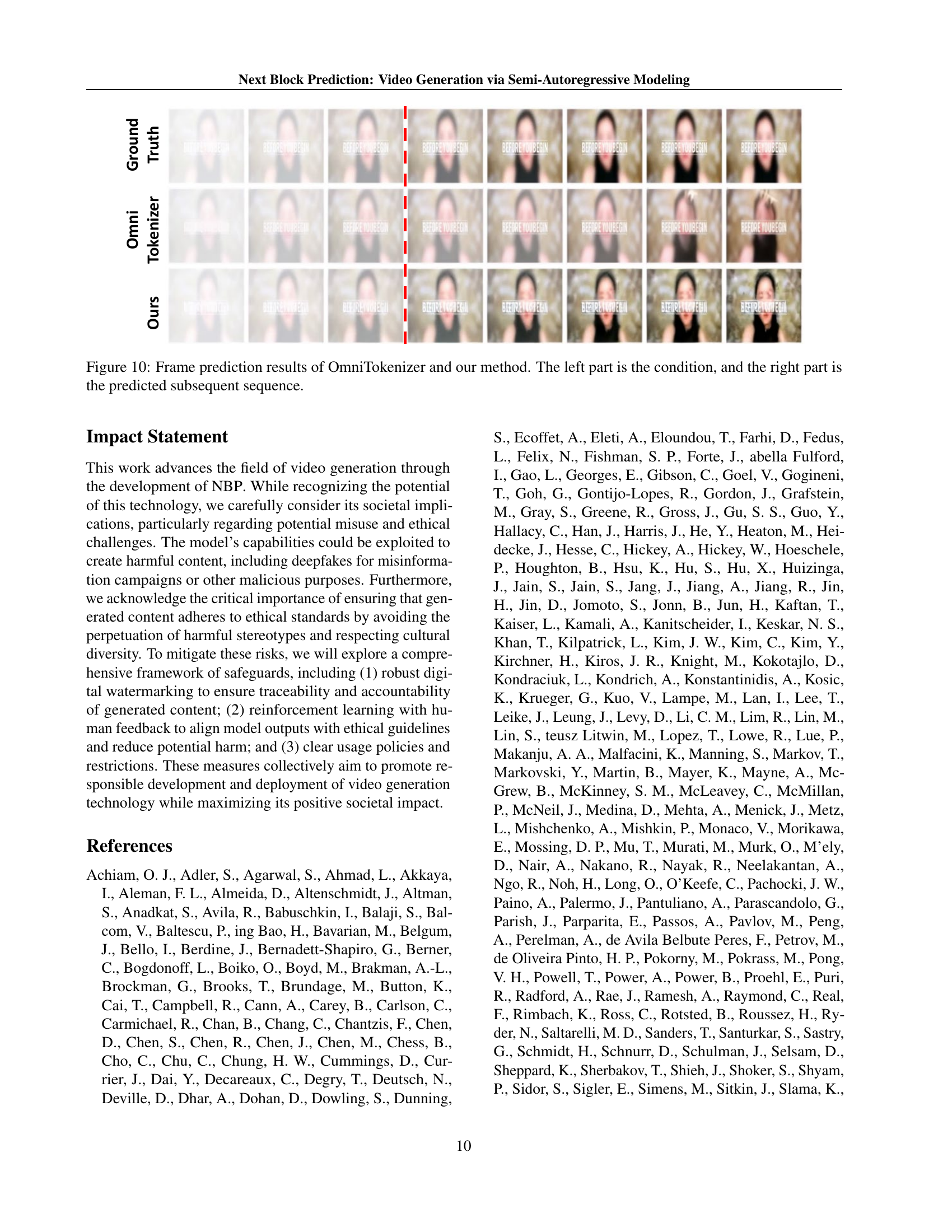
🔼 This figure displays a comparison of frame prediction results between the OmniTokenizer method and the Next-Block Prediction (NBP) method proposed in the paper. The left side shows the input frames (the ‘condition’), a short video sequence used to initiate the prediction. The right side shows the generated frames (the ‘predicted subsequent sequence’) which are the frames predicted by each method. By comparing the generated frames with the ground truth, one can visually assess the performance of each method in terms of accuracy and quality in video prediction tasks. The differences between the OmniTokenizer and NBP predictions highlight the improvements achieved by the NBP model.
read the caption
Figure 10: Frame prediction results of OmniTokenizer and our method. The left part is the condition, and the right part is the predicted subsequent sequence.

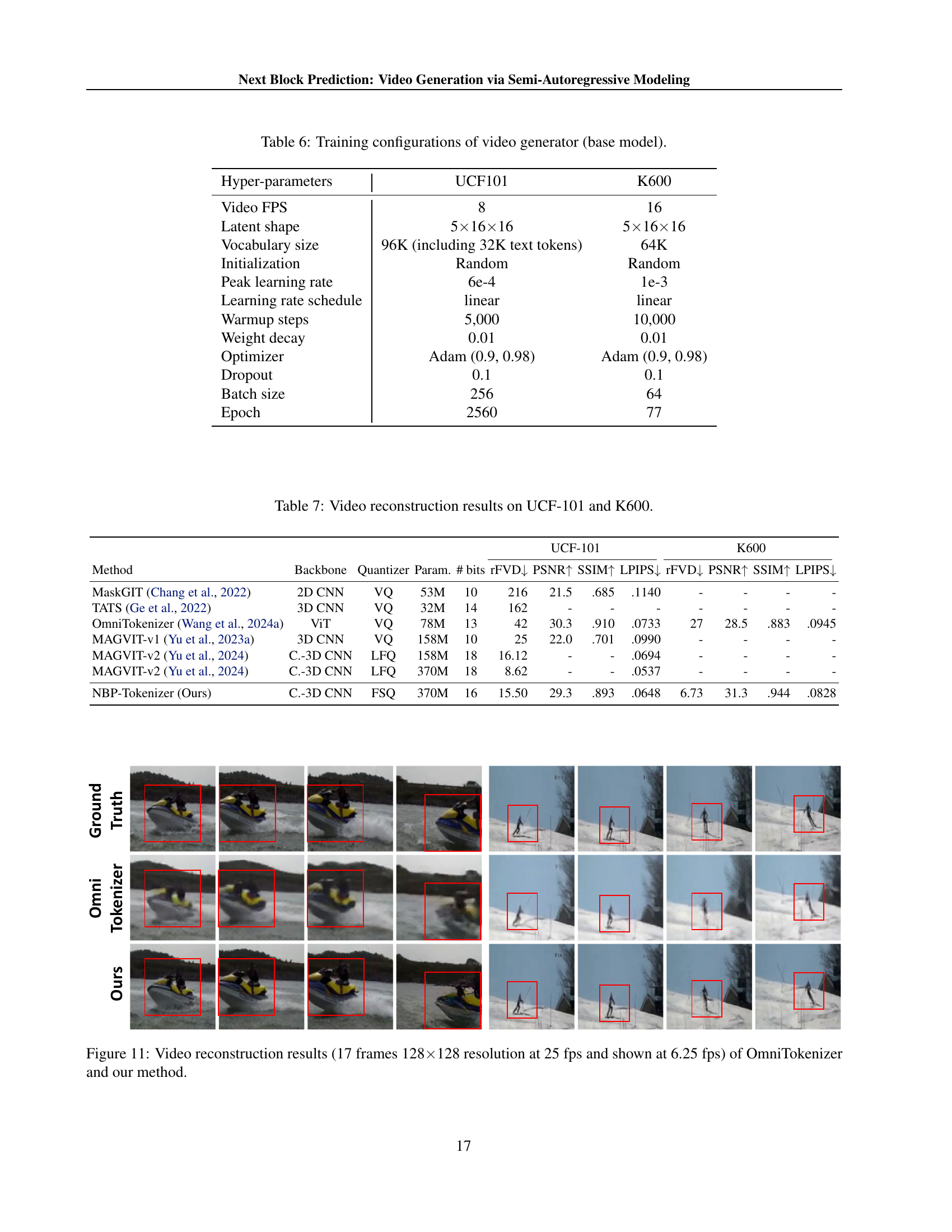
🔼 This figure presents a comparison of video reconstruction results between the OmniTokenizer method and the Next Block Prediction (NBP) method proposed in the paper. It shows sample video frames (17 frames total, 128x128 resolution) generated by each method to illustrate the visual quality differences. The original video is displayed at 25 frames per second (fps), but for easier viewing within the figure, the frames are displayed at 6.25 fps. A visual inspection allows one to assess the level of detail, artifacts, and overall reconstruction accuracy achieved by each method.
read the caption
Figure 11: Video reconstruction results (17 frames 128×\times×128 resolution at 25 fps and shown at 6.25 fps) of OmniTokenizer and our method.

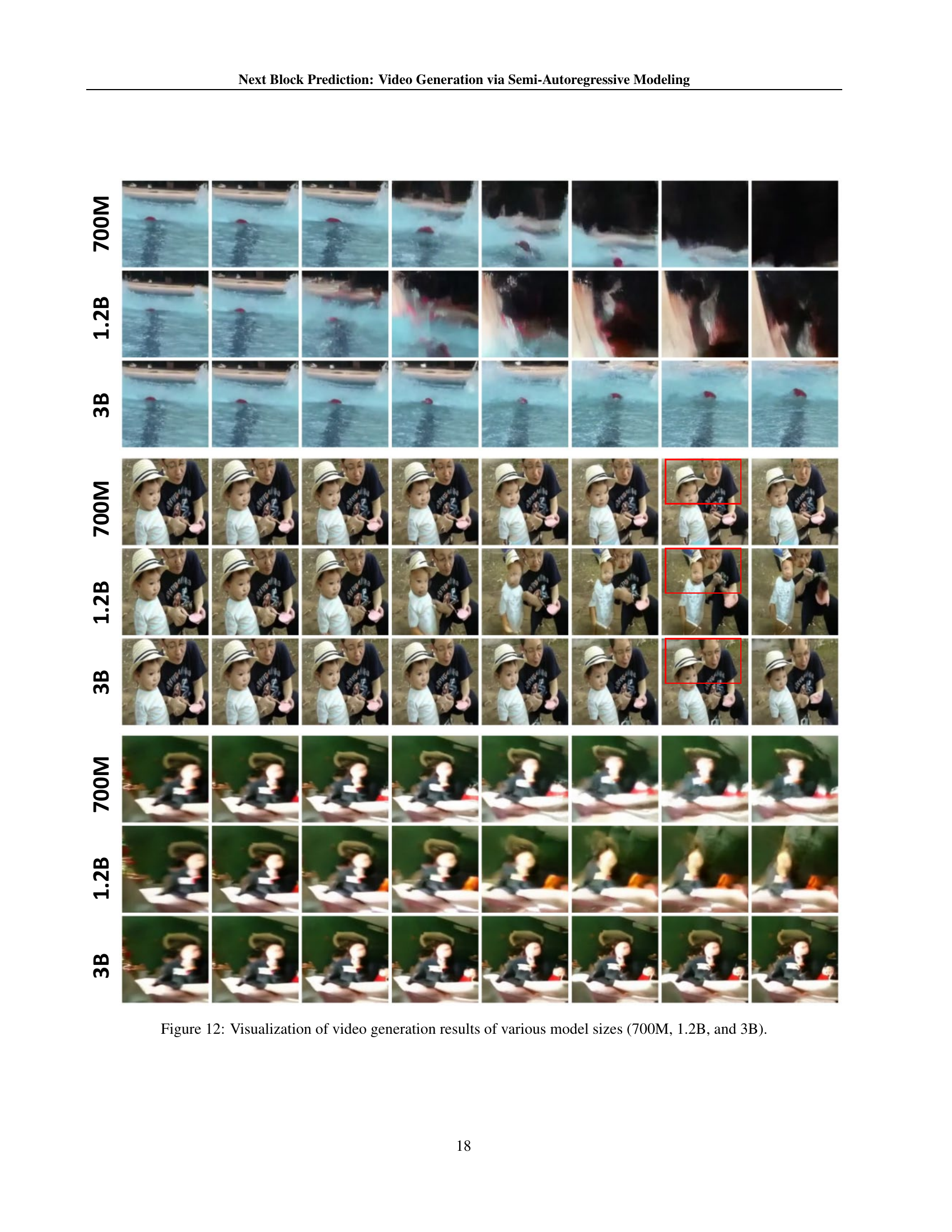
🔼 This figure displays video generation results from three different sized models: 700 million parameters, 1.2 billion parameters, and 3 billion parameters. Each row shows a different video generated by each model. The purpose is to demonstrate how increasing model size impacts the quality of generated videos. Observe the visual details to compare and contrast the outputs of the three models. The generated videos shown exemplify the ability of the model to generate different video clips.
read the caption
Figure 12: Visualization of video generation results of various model sizes (700M, 1.2B, and 3B).

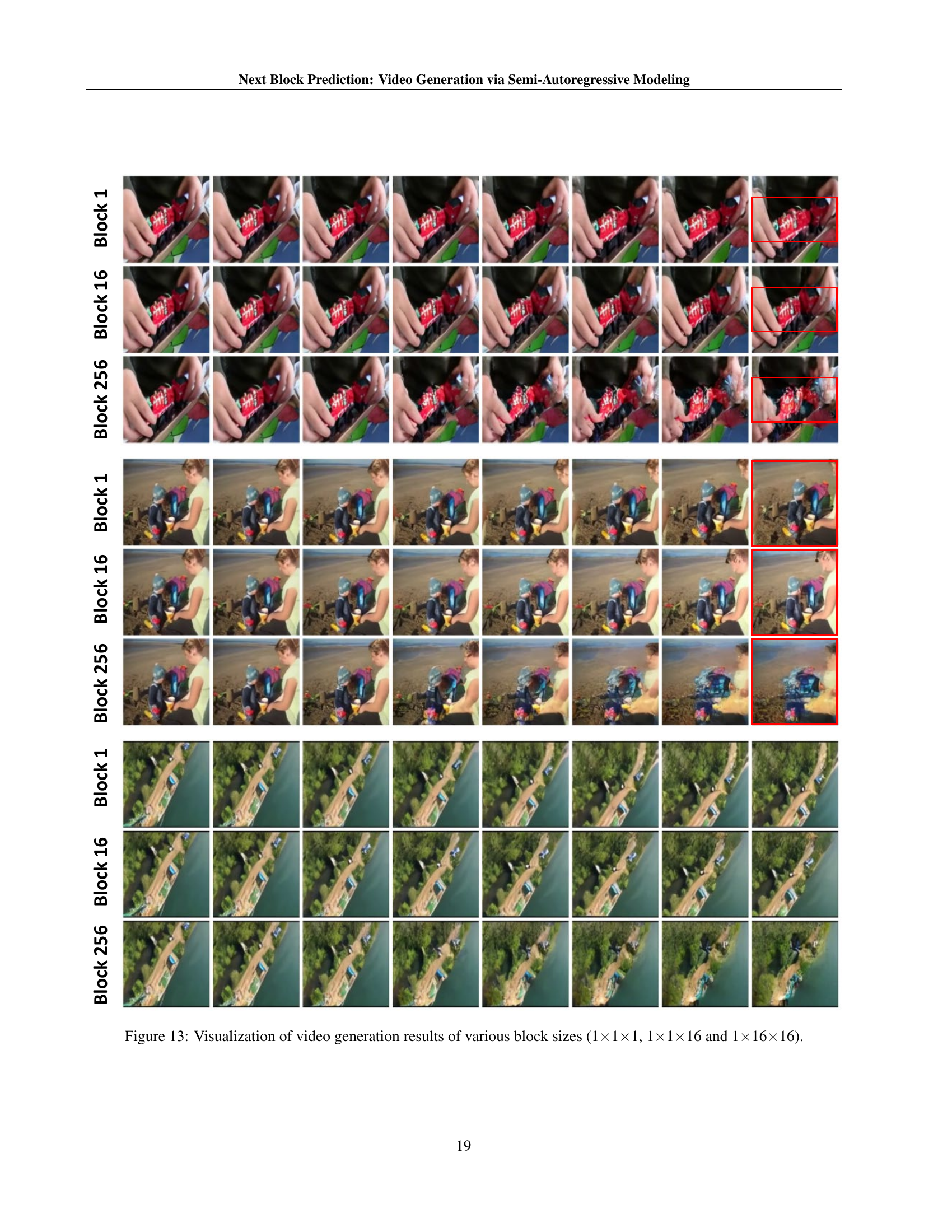
🔼 This figure visualizes the video generation results using different block sizes within the Next-Block Prediction (NBP) model. It shows three sets of video generation outputs, each corresponding to a different block size: 1x1x1 (token-wise), 1x1x16 (row-wise), and 1x1x16 (a larger block spanning multiple tokens). The three rows represent three different sample videos. The aim is to illustrate how altering the size of the processing unit (block size) impacts the model’s ability to generate coherent and visually accurate video sequences.
read the caption
Figure 13: Visualization of video generation results of various block sizes (1×\times×1×\times×1, 1×\times×1×\times×16 and 1×\times×16×\times×16).

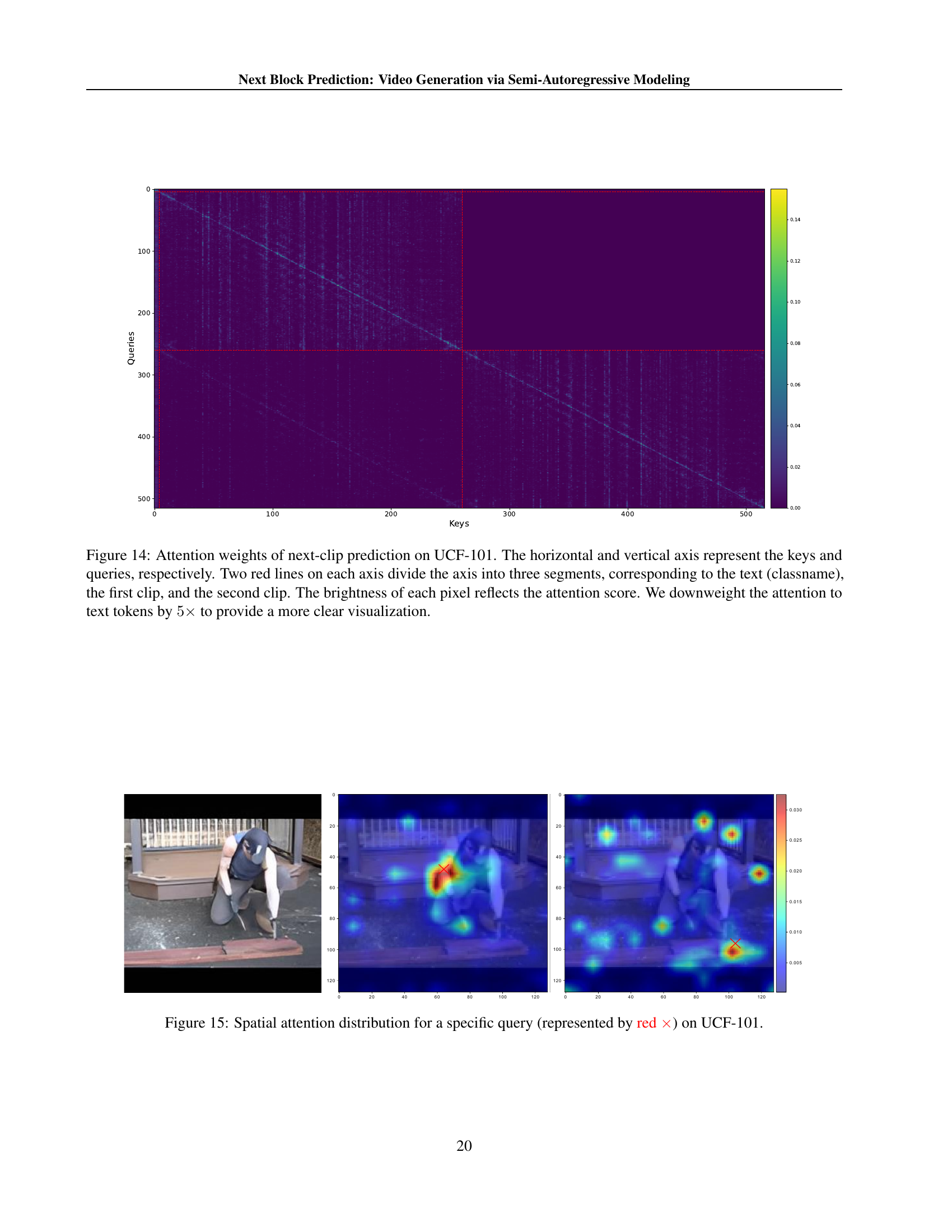
🔼 Figure 14 is a heatmap visualizing the attention weights within the model during the next-clip prediction task on the UCF-101 dataset. The x and y axes represent the keys and queries, respectively, with each axis divided into three segments by two red lines: the text (class name), the first video clip, and the second video clip. Each pixel’s brightness corresponds to the attention weight between a specific key and query. The attention weights for text tokens are downweighted by a factor of 5 to enhance visualization clarity, highlighting the attention relationships between the textual description, the previous video clip, and the model’s prediction for the next clip.
read the caption
Figure 14: Attention weights of next-clip prediction on UCF-101. The horizontal and vertical axis represent the keys and queries, respectively. Two red lines on each axis divide the axis into three segments, corresponding to the text (classname), the first clip, and the second clip. The brightness of each pixel reflects the attention score. We downweight the attention to text tokens by 5×5\times5 × to provide a more clear visualization.

🔼 Figure 15 visualizes the spatial attention distribution within the Next-Block Prediction (NBP) model for a single query token (marked in red). It shows how the attention mechanism weights the relevance of different spatial locations within the video frame when predicting the corresponding token in the next block. This illustrates the model’s ability to capture spatial dependencies and relationships across the frame, a key improvement over traditional autoregressive models that rely on unidirectional dependencies.
read the caption
Figure 15: Spatial attention distribution for a specific query (represented by red ×\times×) on UCF-101.
More on tables
| Model | Parameters | Layers | Hidden Size | Heads |
|---|---|---|---|---|
| NBP-XL | 700M | 24 | 1536 | 16 |
| NBP-XXL | 1.2B | 24 | 2048 | 32 |
| NBP-3B | 3B | 32 | 3072 | 32 |
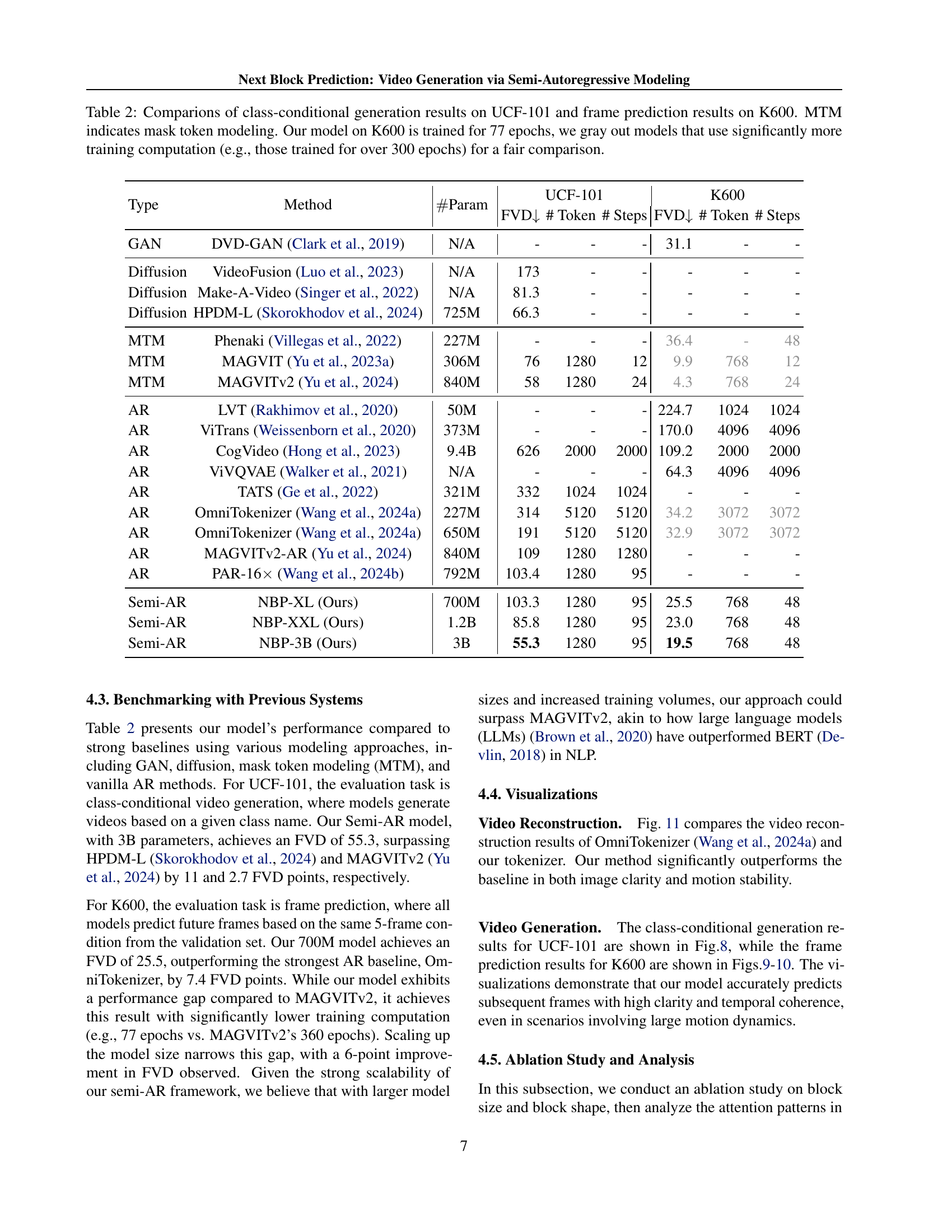
🔼 Table 2 presents a comparison of video generation models’ performance on two benchmark datasets: UCF-101 and Kinetics-600. For UCF-101, the task is class-conditional video generation, where the model generates videos based on a given class label. For Kinetics-600, the task is frame prediction, where the model predicts future frames given a sequence of initial frames. The table includes various models from different categories, including GANs, diffusion models, mask token modeling (MTM) approaches, and autoregressive (AR) models. The models are evaluated based on Fréchet Video Distance (FVD), indicating video quality, the number of tokens used, and the number of generation steps required. The table also notes the number of parameters for each model. A key aspect is that models on K600 are assessed fairly, with those trained significantly longer than 77 epochs (e.g., over 300 epochs) grayed out to ensure a fair comparison based on computational resources.
read the caption
Table 2: Comparions of class-conditional generation results on UCF-101 and frame prediction results on K600. MTM indicates mask token modeling. Our model on K600 is trained for 77 epochs, we gray out models that use significantly more training computation (e.g., those trained for over 300 epochs) for a fair comparison.
| Hyper-parameters | UCF101 | K600 |
|---|---|---|
| Video FPS | 8 | 8 |
| Latent shape | 51616 | 51616 |
| Vocabulary size | 64K | 64K |
| Embedding dimension | 6 | 6 |
| Initialization | Random | Random |
| Peak learning rate | 5e-5 | 1e-4 |
| Learning rate schedule | linear | linear |
| Warmup ratio | 0.01 | 0.01 |
| Perceptual loss weight | 0.1 | 0.1 |
| Generator adversarial loss weight | 0.1 | 0.1 |
| Optimizer | Adam | Adam |
| Batch size | 256 | 256 |
| Epoch | 2000 | 100 |
🔼 This table presents an ablation study on the impact of different block shapes on the video generation quality. The experiment uses a 700M parameter model and evaluates various block shapes (T×H×W) such as 1×4×4, 2×1×8, and 1×1×16. The Fréchet Video Distance (FVD) metric is used to assess the quality of generated videos, with lower FVD scores indicating better generation quality. The results show the optimal block shape and its effect on the balance between generation quality and efficiency.
read the caption
Table 3: Generation quality (FVD) of various block shape.
| Hyper-parameters | UCF101 | K600 |
|---|---|---|
| Video FPS | 8 | 16 |
| Latent shape | 51616 | 51616 |
| Vocabulary size | 96K (including 32K text tokens) | 64K |
| Initialization | Random | Random |
| Peak learning rate | 6e-4 | 1e-3 |
| Learning rate schedule | linear | linear |
| Warmup steps | 5,000 | 10,000 |
| Weight decay | 0.01 | 0.01 |
| Optimizer | Adam (0.9, 0.98) | Adam (0.9, 0.98) |
| Dropout | 0.1 | 0.1 |
| Batch size | 256 | 64 |
| Epoch | 2560 | 77 |
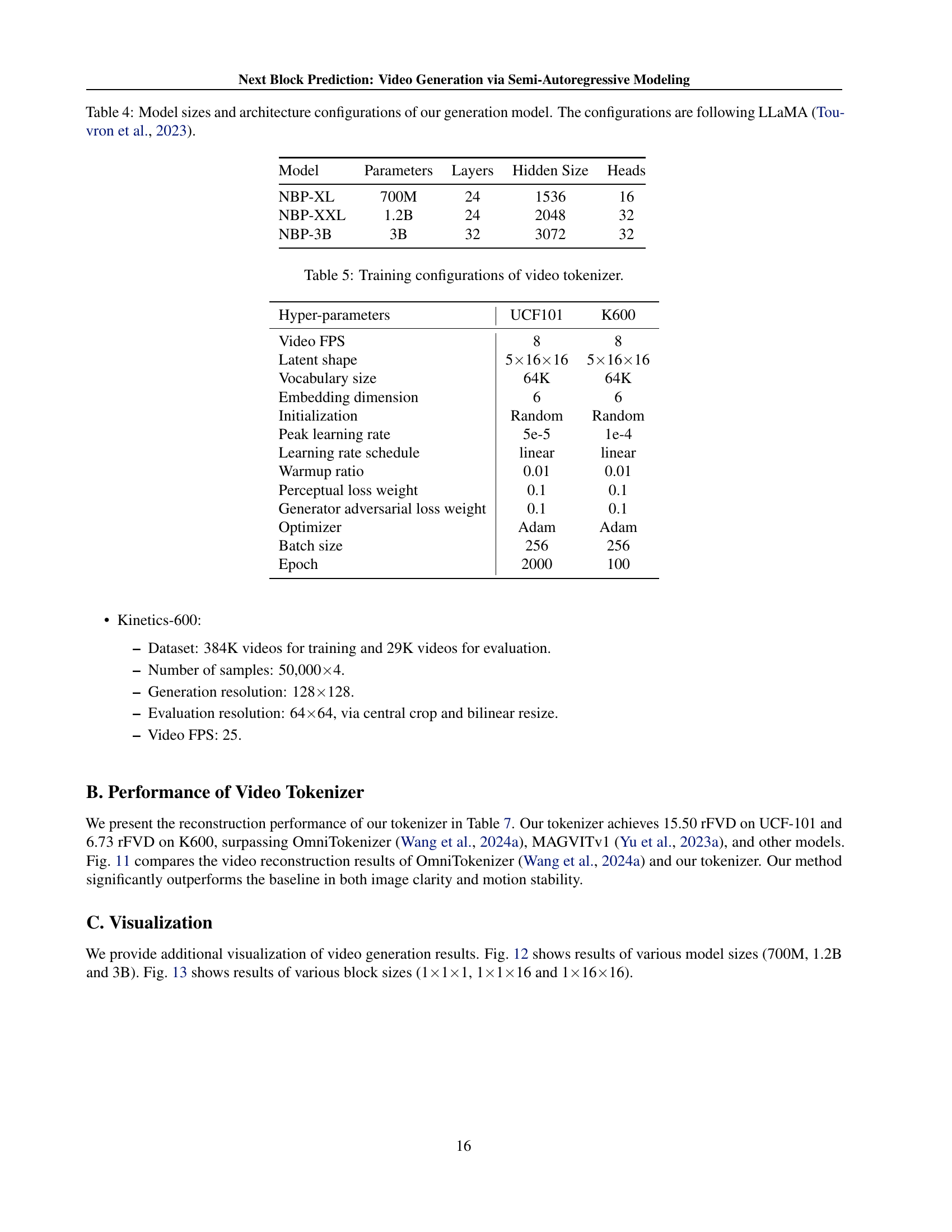
🔼 This table details the different model sizes used in the experiments of the paper. It shows the number of parameters, the number of layers, the hidden size, and the number of attention heads for three different models: NBP-XL, NBP-XXL, and NBP-3B. The architecture of these models follows the LLaMA architecture (Touvron et al., 2023), a well-known large language model architecture.
read the caption
Table 4: Model sizes and architecture configurations of our generation model. The configurations are following LLaMA (Touvron et al., 2023).
| UCF-101 | K600 | |||||||||||
|---|---|---|---|---|---|---|---|---|---|---|---|---|
| Method | Backbone | Quantizer | Param. | # bits | rFVD | PSNR | SSIM | LPIPS | rFVD | PSNR | SSIM | LPIPS |
| MaskGIT (Chang et al., 2022) | 2D CNN | VQ | 53M | 10 | 216 | 21.5 | .685 | .1140 | - | - | - | - |
| TATS (Ge et al., 2022) | 3D CNN | VQ | 32M | 14 | 162 | - | - | - | - | - | - | - |
| OmniTokenizer (Wang et al., 2024a) | ViT | VQ | 78M | 13 | 42 | 30.3 | .910 | .0733 | 27 | 28.5 | .883 | .0945 |
| MAGVIT-v1 (Yu et al., 2023a) | 3D CNN | VQ | 158M | 10 | 25 | 22.0 | .701 | .0990 | - | - | - | - |
| MAGVIT-v2 (Yu et al., 2024) | C.-3D CNN | LFQ | 158M | 18 | 16.12 | - | - | .0694 | - | - | - | - |
| MAGVIT-v2 (Yu et al., 2024) | C.-3D CNN | LFQ | 370M | 18 | 8.62 | - | - | .0537 | - | - | - | - |
| NBP-Tokenizer (Ours) | C.-3D CNN | FSQ | 370M | 16 | 15.50 | 29.3 | .893 | .0648 | 6.73 | 31.3 | .944 | .0828 |
🔼 This table details the hyperparameters used during the training phase of the video tokenizer. It shows the settings specific to both the UCF101 and K600 datasets, including video frames per second (FPS), latent shape of the tokens, vocabulary size, embedding dimension, initialization method, learning rate schedule, peak learning rate, warmup ratio, and optimizer used. It also indicates the perceptual loss weight, generator adversarial loss weight, batch size, and number of epochs used in the training process.
read the caption
Table 5: Training configurations of video tokenizer.
Full paper#