TL;DR#
Large language models (LLMs) learn word representations, but these often suffer from anisotropy, meaning the embeddings are clustered in a small subspace, limiting their semantic usefulness and the model’s overall performance. This anisotropy is a poorly understood phenomenon, but previous research has pointed to a mean embedding vector shift away from the origin as a major contributor.
This paper investigates the role of the Adam optimizer in causing anisotropic embeddings. The authors argue that Adam’s second moment calculation is responsible for the problem. They propose a novel optimizer called Coupled Adam, which modifies the second moment calculation to mitigate anisotropy. Experiments demonstrate that Coupled Adam significantly improves embedding quality and leads to better upstream and downstream performance, especially on larger datasets. The results support the hypothesis that the Adam optimizer contributes significantly to the problem of anisotropic embeddings in LLMs.
Key Takeaways#
Why does it matter?#
This paper is crucial for researchers working with large language models (LLMs) because it addresses a significant problem—anisotropic embeddings—that hinders model performance and generalizability. The proposed Coupled Adam optimizer offers a practical solution, potentially improving the efficiency and effectiveness of LLM training and downstream applications. Further research into the method’s impact on different model architectures and training paradigms would be valuable.
Visual Insights#

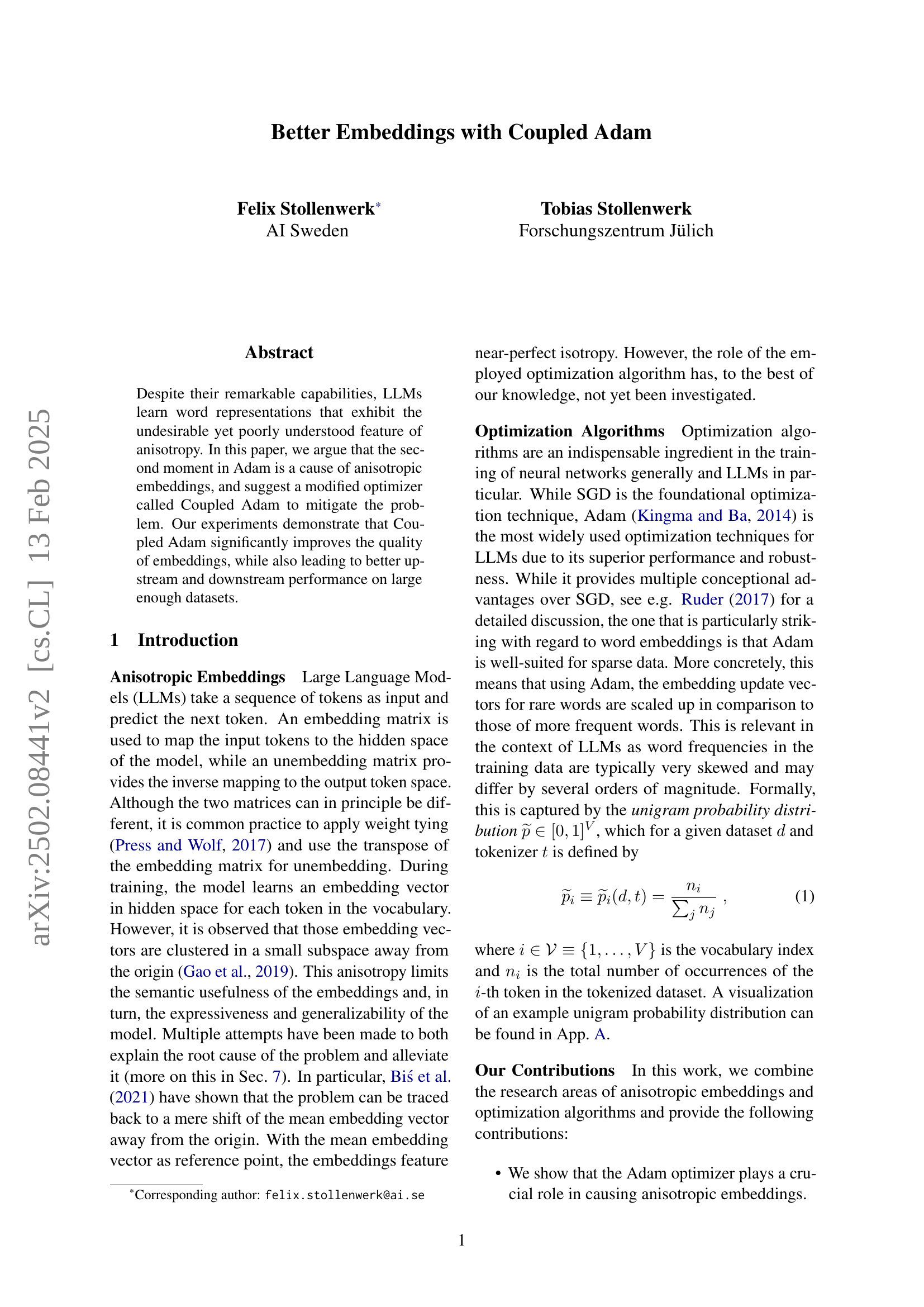
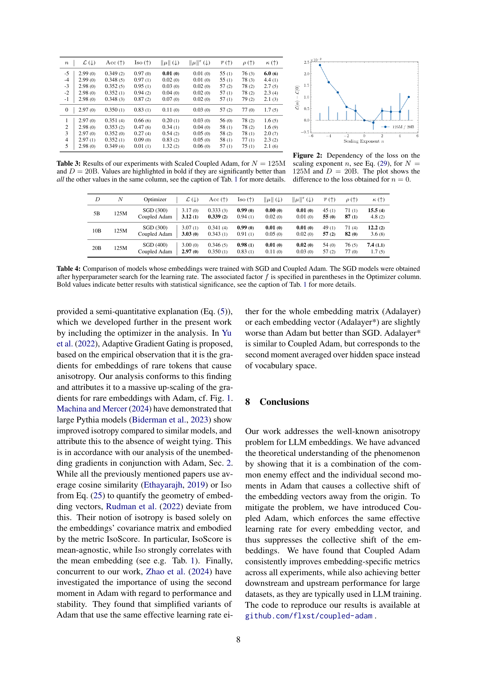
🔼 Figure 1 illustrates the core concept of the paper regarding the anisotropy problem in embedding vectors. It uses a simplified 2D example to visually represent the embedding update vectors for both SGD and Adam optimizers. A hidden state vector (blue) interacts with three embedding vectors (red), one of which corresponds to the correct token. The gray arrows depict the update vectors for each embedding vector, with SGD producing update vectors that sum to zero (demonstrating a balanced update), and Adam having update vectors that do not sum to zero (implying an unbalanced update and thus the creation of anisotropy). This difference in update vector summation between the optimizers helps to explain why Adam contributes to the anisotropy problem that is the main focus of the paper.
read the caption
Figure 1: Toy example of a hidden state vector hℎhitalic_h (shown in blue) and three embedding vectors eisubscript𝑒𝑖e_{i}italic_e start_POSTSUBSCRIPT italic_i end_POSTSUBSCRIPT (shown in red) in H=2𝐻2H=2italic_H = 2 dimensions. The gray vectors represent the embedding update vectors, for the SGD (dark) and the Adam (light) optimizer. The update vector of the true token is aligned with hℎhitalic_h, while the others point in the opposite direction, see Eq. (5). Note that the sum of embedding update vectors vanishes for SGD, while this is not necessarily the case for Adam, cf. Eqs. (11) and (16).
| Adam | () | () | () | () | () | () | () | () | ||
|---|---|---|---|---|---|---|---|---|---|---|
| \resultsS |
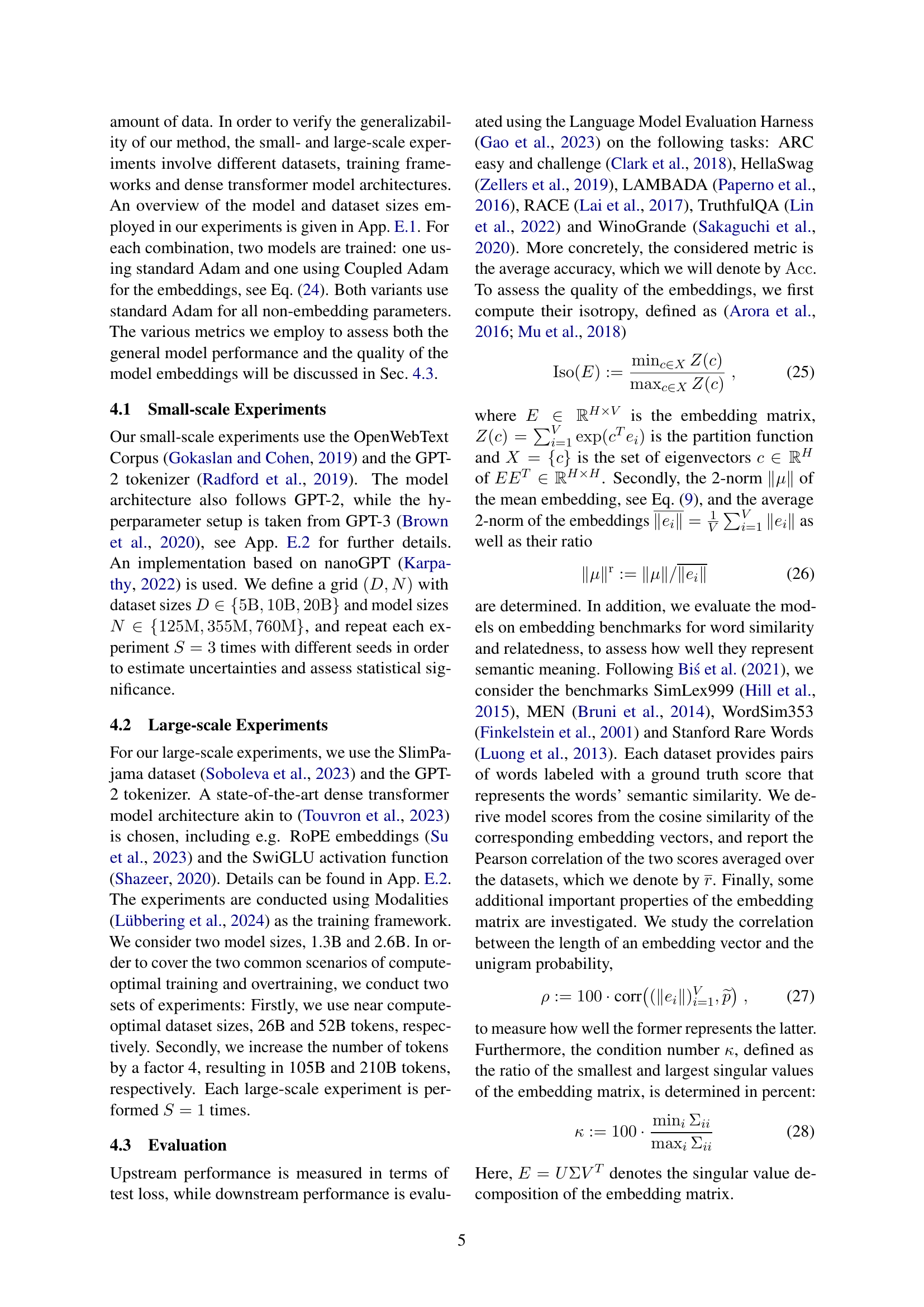
🔼 This table presents the results of small-scale experiments conducted to evaluate the performance of standard Adam and Coupled Adam optimizers. It shows the test loss (ℒ), downstream task accuracy (Acc), isotropy (Iso), mean embedding norm (||μ||), average embedding norm (||ei||), correlation between embedding length and unigram probability (p), and condition number (κ) for various dataset sizes (D) and model sizes (N). Each experiment was repeated three times with different random seeds to assess variability. Statistical significance testing (Student’s t-test with α=0.05) was used to determine whether improvements observed with Coupled Adam are statistically significant, and these results are highlighted in bold. Appendix F details the statistical methodology, while Appendices G.1 shows plots of the loss and downstream task accuracy.
read the caption
Table 1: Results of our small-scale experiments. D𝐷Ditalic_D and N𝑁Nitalic_N denote the dataset and model size, respectively. ℒℒ\mathcal{L}caligraphic_L is the test loss, and the column AccAcc\rm Accroman_Acc represents the accuracy averaged over the downstream tasks listed in Sec. 4.3. The other evaluation metrics are defined in the same section, see Eqs. (25)-(28). The arrow in parentheses indicates whether a higher or lower value is desirable. Every training was conducted S=3𝑆3S=3italic_S = 3 times with different seeds, and the numbers represent the (rounded) averages and standard deviations in the following shorthand notation format: 0.1230.1230.1230.123 (4)4(4)( 4 ) ≡0.123±0.004absentplus-or-minus0.1230.004\equiv 0.123\pm 0.004≡ 0.123 ± 0.004. For each combination (D,N)𝐷𝑁(D,N)( italic_D , italic_N ) and each metric, the respective better value is highlighted in bold if the (unrounded) difference is significant according to Student’s t-test with a one-sided confidence level of α=95%𝛼percent95\alpha=95\%italic_α = 95 % (see App. F for details). Plots for ℒℒ\mathcal{L}caligraphic_L and AccAcc\rm Accroman_Acc are shown in App. G.1.
In-depth insights#
Adam’s Anisotropy#
The concept of “Adam’s Anisotropy” encapsulates the observation that the Adam optimizer, while highly effective for training large language models (LLMs), contributes to the undesirable phenomenon of anisotropic word embeddings. Anisotropy in this context refers to the uneven distribution of embedding vectors in the model’s hidden space; they tend to cluster in a restricted subspace rather than being uniformly dispersed. This unevenness is problematic because it limits the semantic richness and generalizability of the model’s representations. The paper explores this issue by analyzing the mathematical properties of the Adam update rule and its interactions with the unique characteristics of LLM training data (i.e., highly skewed word frequency distributions). The core argument revolves around how Adam’s second-moment estimate (v) scales embedding updates differently for frequent versus rare words, leading to the anisotropic clustering. The authors propose “Coupled Adam,” a modification to Adam designed to mitigate this issue by ensuring more uniform scaling of updates, thus resulting in more isotropic and improved embeddings. Empirical evidence demonstrates that this modification significantly improves both the quality of word embeddings and downstream performance.
Coupled Adam#
The proposed “Coupled Adam” optimization algorithm addresses the anisotropy problem in large language model (LLM) embeddings. Anisotropy, where embedding vectors cluster in a limited subspace, hinders model expressiveness and generalizability. The core idea is that the standard Adam optimizer’s second moment, used for normalization, contributes to this issue. By coupling the second moments of all embedding vectors, the algorithm ensures that the effective learning rate is consistent across all parameters. This prevents the over-scaling of updates for less frequent words, a factor identified as a main cause of anisotropy. The results demonstrate that Coupled Adam improves both the quality of embeddings and the model’s performance on large datasets, achieving better isotropy and downstream performance while mitigating the problem of the mean embedding shifting away from the origin. The method is efficient and easy to implement, requiring only minor changes to existing Adam implementations. Further investigation explores the impact of scaling the coupled second moment, indicating that maintaining a consistent learning rate across embedding parameters yields optimal results.
Embedding Metrics#
Embedding metrics are crucial for evaluating the quality of learned word representations in language models. Effective metrics should capture the semantic relationships between words, assessing both the accuracy and generalizability of the embeddings. Common approaches involve measuring the distance between embedding vectors to reflect semantic similarity, potentially using techniques like cosine similarity. However, simply evaluating pairwise similarity is insufficient; a good metric should also assess the global structure of the embedding space, looking for undesirable properties like anisotropy (where the embeddings are clustered in a small subspace). Isotropy is often used as a measure of embedding quality, indicating that the distribution of vectors is uniform in the high-dimensional space. Beyond these standard approaches, metrics can also consider the correlation between embedding properties and external factors like word frequency or human judgments of semantic similarity. Ultimately, the choice of metrics depends on the specific research goals and the nature of the downstream task; no single metric perfectly captures all relevant aspects of embedding quality.
Large-Scale Tests#
A dedicated section on ‘Large-Scale Tests’ within a research paper would be crucial for validating the generalizability and robustness of proposed methods. It would need to go beyond small-scale experiments, employing significantly larger datasets and more complex models to ensure findings aren’t artifacts of limited scope. The section should detail the specific datasets used, their sizes and characteristics (e.g., distribution, noise levels), as well as the architecture and parameter counts of the models tested. Computational resources used for these tests would also warrant mention. The results should focus on both quantitative metrics (e.g., accuracy, loss, isotropy) and qualitative observations about model behavior. Crucially, the large-scale tests should address the scalability of the method, analyzing how performance changes with increased data and model complexity. This could involve comparing the method’s efficiency and resource requirements against alternatives. Finally, a discussion of the consistency of findings between small and large-scale experiments, highlighting any differences or limitations, is vital for establishing confidence in the method’s broader applicability.
Future Work#
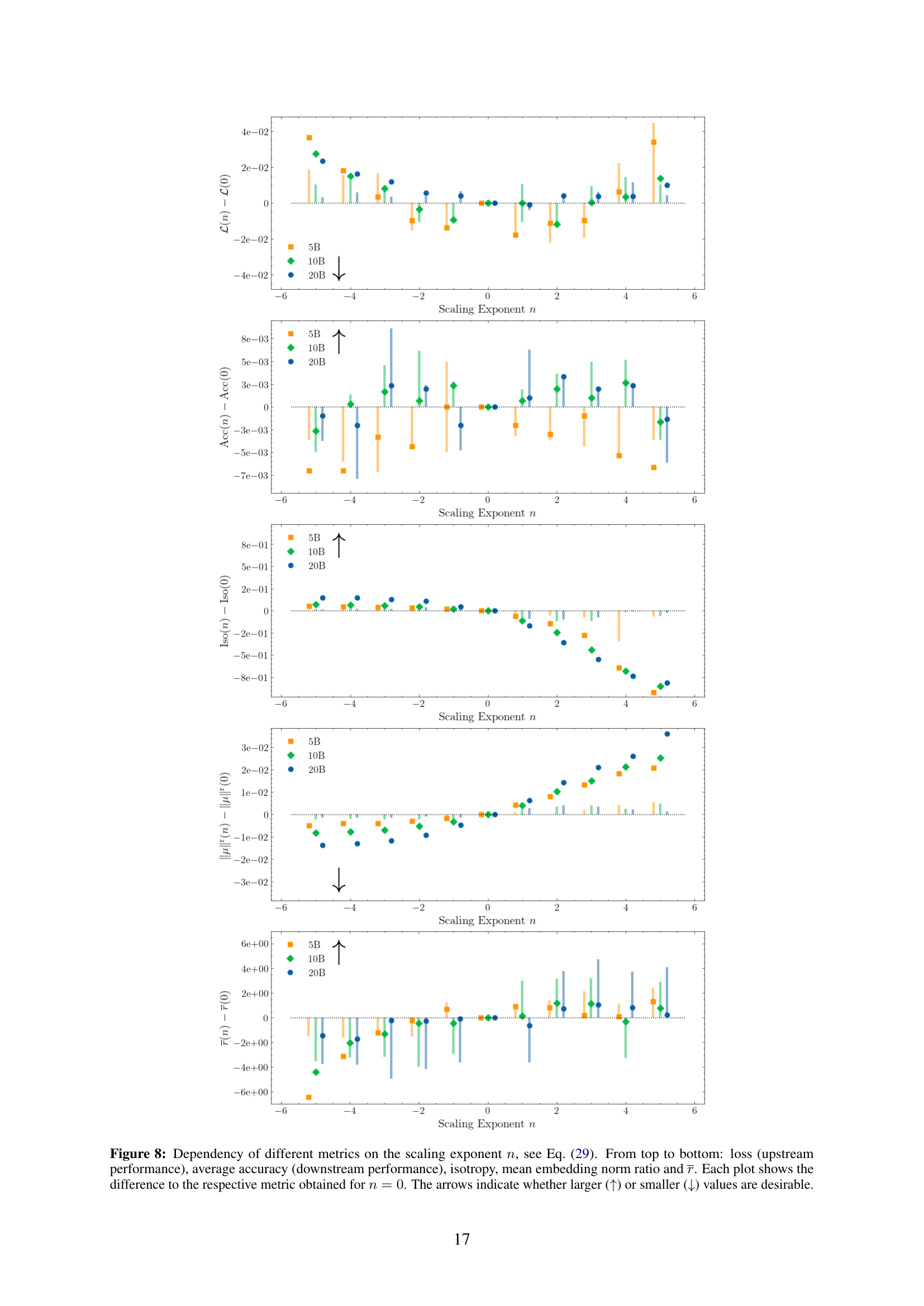
The paper’s ‘Future Work’ section presents exciting avenues for extending this research. Investigating the impact of weight tying on the observed mean embedding shift is crucial, as it may explain the residual anisotropy even with Coupled Adam. Exploring alternative learning rate schedules, beyond the cosine decay used, could reveal further performance improvements. More sophisticated Coupled Adam implementations are also warranted, potentially enhancing efficiency and effectiveness. Finally, extending the experiments to models beyond 2.6B parameters is essential to confirm the generalizability of the proposed approach across larger, more complex LLMs. These directions would significantly advance the understanding of anisotropic embeddings and the optimization strategies necessary to address this critical problem in large language models.
More visual insights#
More on figures

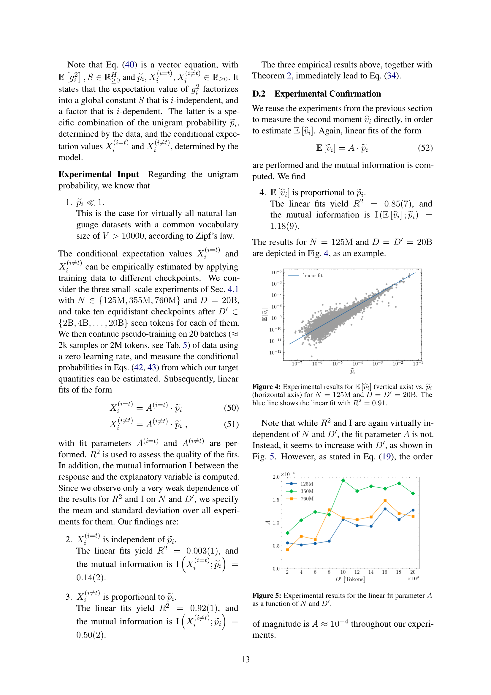
🔼 This figure displays the relationship between the expected value of the embedding update vector’s squared magnitude (𝔼[v^i]) and the unigram probability (p
i) for a specific model size (N=125M) and dataset size (D=20B). Each point represents an embedding vector, and its vertical position indicates the expected value of the squared magnitude of its update vector, while its horizontal position shows its corresponding unigram probability. The blue line is a linear fit through the data points, showing a strong positive correlation (R²=0.91). This visualization helps to demonstrate that embeddings of more frequent words (higher pi) tend to have smaller updates (lower 𝔼[v^i]), and vice versa, which is crucial for understanding the effects of Adam optimization on anisotropic embeddings.read the caption
Figure 4: Experimental results for 𝔼[v^i]𝔼delimited-[]subscript^𝑣𝑖\mathbb{E}\left[\widehat{v}_{i}\right]blackboard_E [ over^ start_ARG italic_v end_ARG start_POSTSUBSCRIPT italic_i end_POSTSUBSCRIPT ] (vertical axis) vs. p~isubscript~𝑝𝑖\widetilde{p}_{i}over~ start_ARG italic_p end_ARG start_POSTSUBSCRIPT italic_i end_POSTSUBSCRIPT (horizontal axis) for N=125M𝑁125MN=125\rm Mitalic_N = 125 roman_M and D=D′=20B𝐷superscript𝐷′20BD=D^{\prime}=20\rm Bitalic_D = italic_D start_POSTSUPERSCRIPT ′ end_POSTSUPERSCRIPT = 20 roman_B. The blue line shows the linear fit with R2=0.91superscript𝑅20.91R^{2}=0.91italic_R start_POSTSUPERSCRIPT 2 end_POSTSUPERSCRIPT = 0.91.

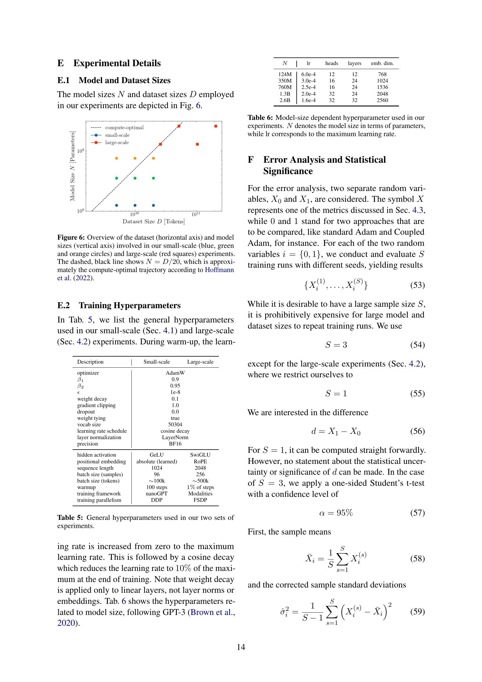
🔼 This figure displays the results of linear fits performed to experimentally determine the proportionality constant A in the relationship E[vᵢ] ≈ A⋅pᵢ, where E[vᵢ] is the expectation value of the Adam optimizer’s second moment for the i-th embedding vector and pᵢ is the unigram probability of the i-th token. The graph shows how the fitted parameter A varies with model size (N) and the amount of training data (D’). Different colors represent different model sizes, demonstrating that the relationship between A and D’ is dependent upon model size. This helps to understand the influence of model size and training dataset size on the anisotropy issue.
read the caption
Figure 5: Experimental results for the linear fit parameter A𝐴Aitalic_A as a function of N𝑁Nitalic_N and D′superscript𝐷′D^{\prime}italic_D start_POSTSUPERSCRIPT ′ end_POSTSUPERSCRIPT.

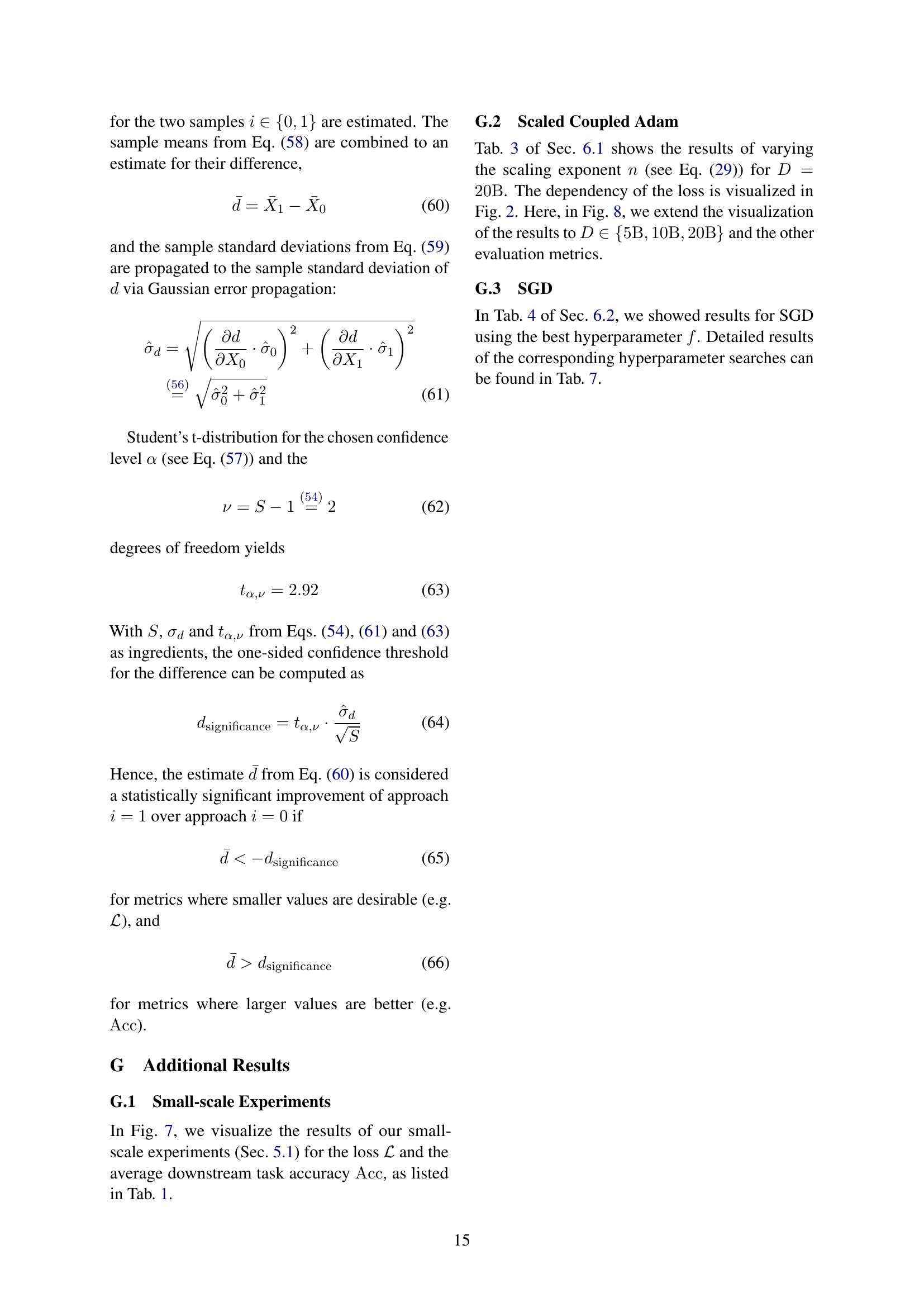
🔼 Figure 6 shows the relationship between dataset size and model size used in the experiments. The horizontal axis represents the size of the dataset (D, in tokens), and the vertical axis represents the size of the model (N, in parameters). Small-scale experiments are represented by blue, green, and orange circles, while large-scale experiments are shown as red squares. The dashed black line illustrates the compute-optimal trajectory proposed by Hoffmann et al. (2022), suggesting an approximate ratio of dataset size to model size (D/N) of 20. This line serves as a reference point to compare the dataset and model sizes used in the study.
read the caption
Figure 6: Overview of the dataset (horizontal axis) and model sizes (vertical axis) involved in our small-scale (blue, green and orange circles) and large-scale (red squares) experiments. The dashed, black line shows N=D/20𝑁𝐷20N=D/20italic_N = italic_D / 20, which is approximately the compute-optimal trajectory according to hoffmann2022trainingcomputeoptimallargelanguage.
More on tables
| Adam | () | () | () | () | () | () | () | () | ||
|---|---|---|---|---|---|---|---|---|---|---|
| \resultsL |
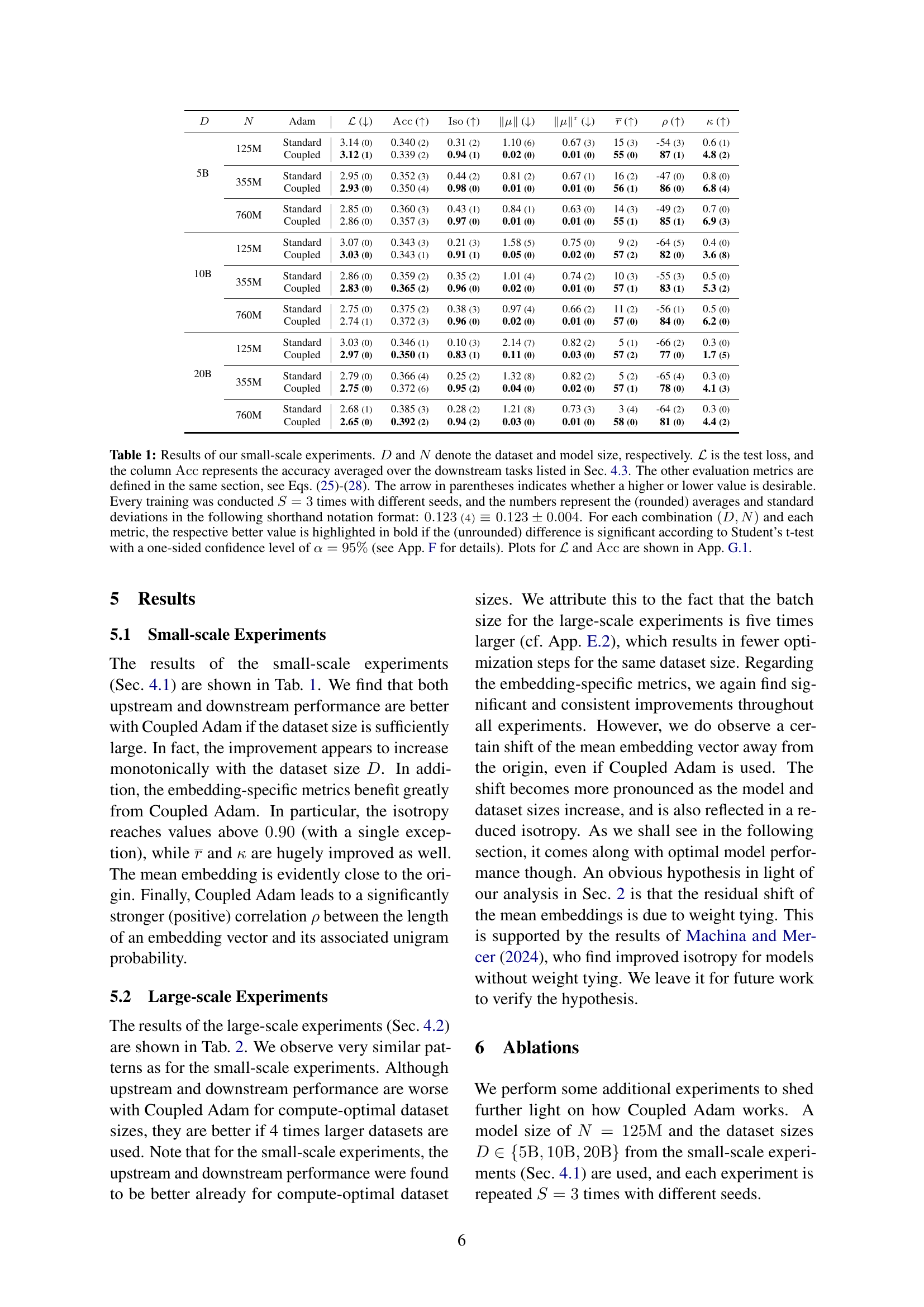
🔼 This table presents the results of large-scale experiments conducted in the paper. It compares the performance of models trained using standard Adam and Coupled Adam optimizers on different dataset sizes (D) and model sizes (N). The metrics used to evaluate performance are: test loss (L), average accuracy across downstream tasks (Acc), isotropy (Iso), the 2-norm of the mean embedding vector (||µ||), the average 2-norm of the embedding vectors (||ei||), the correlation between embedding vector length and unigram probability (p), and the condition number (κ). For each combination of dataset and model size and each metric, the better result (either higher or lower value depending on the metric) is highlighted in bold, indicating statistical significance.
read the caption
Table 2: Results of our large-scale experiments. See the caption of Tab. 4.3 for an explanation of the column names. For each combination (D,N)𝐷𝑁(D,N)( italic_D , italic_N ) and each metric, the respective better value is highlighted in bold.
| Description | Small-scale | Large-scale |
|---|---|---|
| optimizer | AdamW | |
| 0.9 | ||
| 0.95 | ||
| 1e-8 | ||
| weight decay | 0.1 | |
| gradient clipping | 1.0 | |
| dropout | 0.0 | |
| weight tying | true | |
| vocab size | 50304 | |
| learning rate schedule | cosine decay | |
| layer normalization | LayerNorm | |
| precision | BF16 | |
| hidden activation | GeLU | SwiGLU |
| positional embedding | absolute (learned) | RoPE |
| sequence length | 1024 | 2048 |
| batch size (samples) | 96 | 256 |
| batch size (tokens) | 100k | 500k |
| warmup | 100 steps | of steps |
| training framework | nanoGPT | Modalities |
| training parallelism | DDP | FSDP |
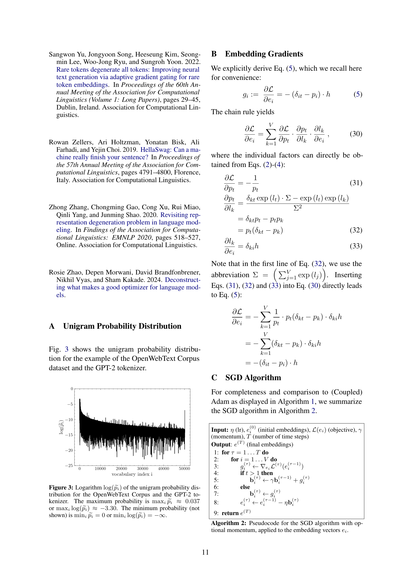
🔼 This table presents the pseudocode for the Stochastic Gradient Descent (SGD) algorithm, a common optimization method in machine learning. It details how SGD updates the embedding vectors (ei) in a language model. The algorithm includes an optional momentum term (γ) to accelerate convergence and smooth out the updates. The input includes the learning rate (η), the initial embedding vectors, the objective function (L), and the number of timesteps (T). The output is the final set of embedding vectors after training.
read the caption
Algorithm 2 Pseudocode for the SGD algorithm with optional momentum, applied to the embedding vectors eisubscript𝑒𝑖e_{i}italic_e start_POSTSUBSCRIPT italic_i end_POSTSUBSCRIPT.
| lr | heads | layers | emb. dim. | |
|---|---|---|---|---|
| 124M | 6.0e-4 | 12 | 12 | 768 |
| 350M | 3.0e-4 | 16 | 24 | 1024 |
| 760M | 2.5e-4 | 16 | 24 | 1536 |
| 1.3B | 2.0e-4 | 32 | 24 | 2048 |
| 2.6B | 1.6e-4 | 32 | 32 | 2560 |
🔼 This table lists the general hyperparameters used in the small-scale and large-scale experiments described in the paper. It includes settings for both the optimizer (AdamW), its hyperparameters (betas, weight decay, gradient clipping), embedding parameters (dropout, weight tying, vocabulary size), and training parameters (learning rate schedule, layer normalization, precision, activation function, positional embedding, sequence length, batch size (samples and tokens), and warmup steps. The training framework (nanoGPT vs. Modalities) and training parallelism (DDP vs. FSDP) are also specified.
read the caption
Table 5: General hyperparameters used in our two sets of experiments.
| Optimizer | () | () | () | () | () | () | () | () | ||
|---|---|---|---|---|---|---|---|---|---|---|
| \resultsAblationsSGDExpFive |
🔼 This table shows the hyperparameter settings used in the experiments for different model sizes. The hyperparameters are those that change depending on the model size, and exclude those which remain constant across experiments. Key hyperparameters listed include the model size (in number of parameters), maximum learning rate, number of attention heads, number of layers in the model, and embedding dimension.
read the caption
Table 6: Model-size dependent hyperparameter used in our experiments. N𝑁Nitalic_N denotes the model size in terms of parameters, while lr corresponds to the maximum learning rate.
| Optimizer | () | () | () | () | () | () | () | () | ||
|---|---|---|---|---|---|---|---|---|---|---|
| \resultsAblationsSGDExpTen |
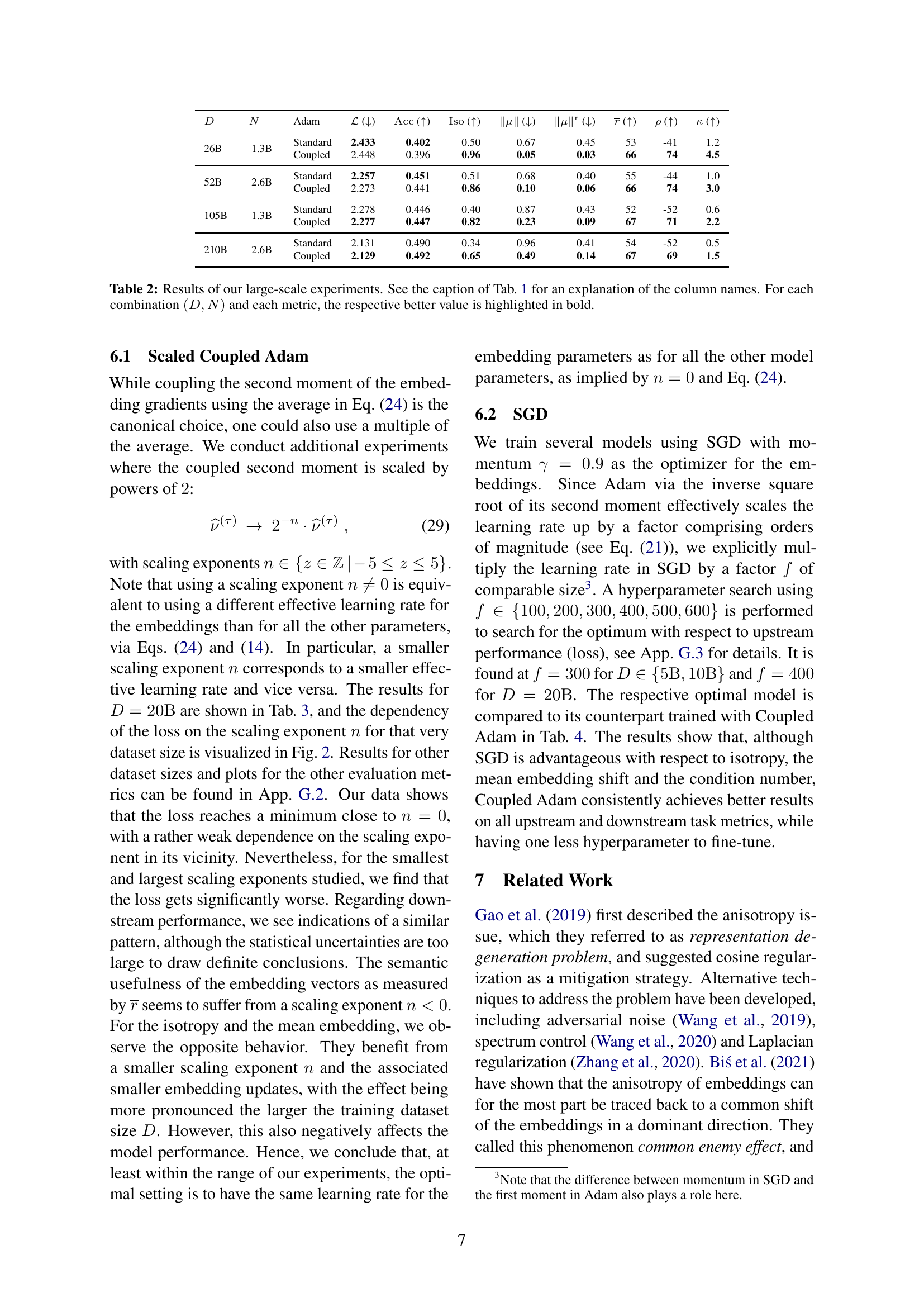
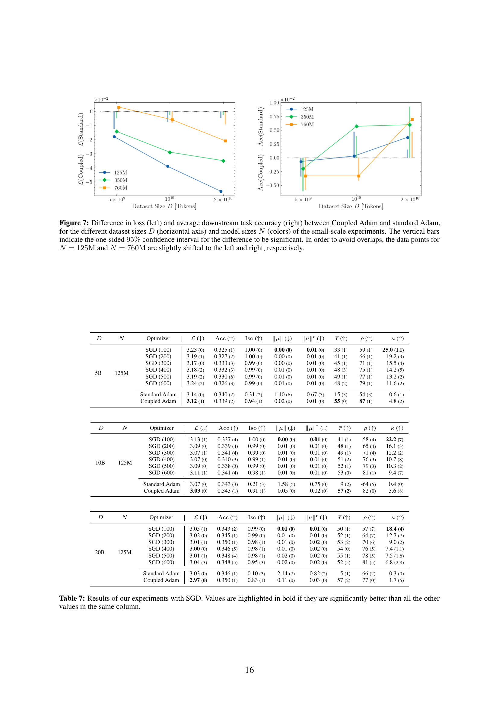
🔼 This table presents the results of experiments using Stochastic Gradient Descent (SGD) as the optimizer for word embeddings, comparing it against Coupled Adam. It shows the test loss, downstream task accuracy (averaged across multiple tasks), isotropy, mean embedding norm, average embedding norm, the correlation between embedding length and unigram probability, and the embedding matrix’s condition number. For each metric, the best performing model is highlighted in bold, indicating statistically significant improvements over other configurations. The experiments were conducted with different dataset and model sizes.
read the caption
Table 7: Results of our experiments with SGD. Values are highlighted in bold if they are significantly better than all the other values in the same column.
Full paper#