Cluster and Predict Latents Patches for Improved Masked Image Modeling

2502.08769

Timothée Darcet et el.

🤗 2025-02-17

TL;DR
#

Current Masked Image Modeling (MIM) methods for self-supervised visual representation learning lag behind state-of-the-art techniques. Existing MIM approaches suffer from issues such as instability during training and poor representation quality when compared to other self-supervised methods. These limitations hinder the development of robust foundation models capable of excelling in various computer vision tasks.

This paper introduces CAPI, a novel MIM framework that addresses these challenges. CAPI uses a clustering-based loss function that is more stable during training and leads to improved representation quality. The method achieves state-of-the-art results on benchmark datasets (ImageNet and ADE20K), significantly outperforming previous MIM methods while approaching the performance of the current top performer, DINOv2. The proposed approach offers a promising direction for future research in self-supervised learning and the development of powerful foundation models for computer vision.

Key Takeaways
#

Why does it matter?
#

This paper is crucial for researchers in computer vision and self-supervised learning. It significantly advances masked image modeling, a key area in self-supervised representation learning. The paper’s focus on improving the stability and effectiveness of MIM, along with its strong empirical results, opens new avenues for research in creating better foundation models and self-supervised learning techniques that are more scalable and efficient. Its proposed method, CAPI, achieves state-of-the-art results, demonstrating a clear advancement in the field.

Visual Insights
#

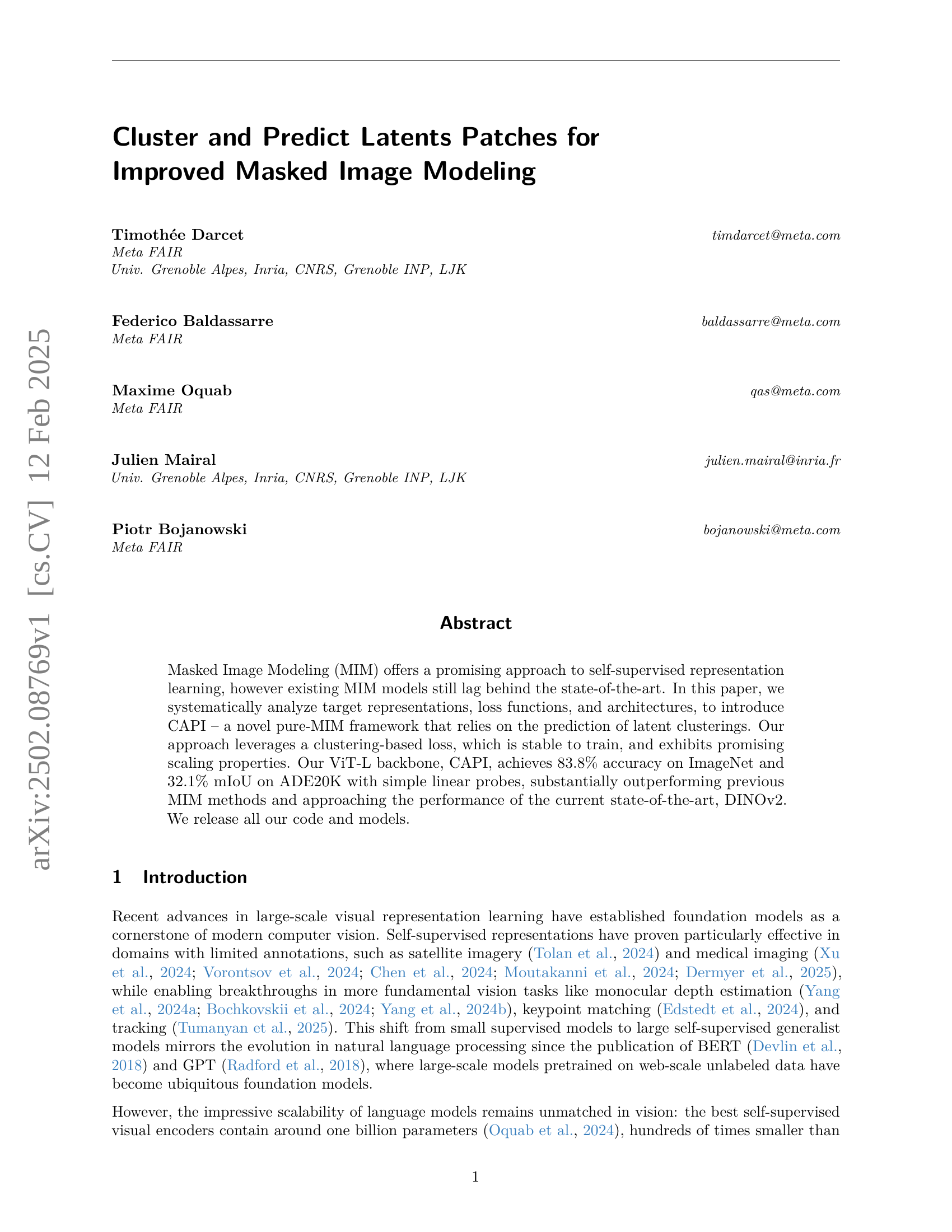
🔼 This figure illustrates the CAPI method, a novel approach to masked image modeling. Image patches are processed by a teacher network, which then groups them into clusters based on latent representations. These cluster assignments serve as the training signal for a student network, trained via self-distillation with the teacher. Notably, the loss function focuses solely on predicting the content of masked image patches, without relying on augmentations or contrastive learning. The figure then shows performance comparisons against existing methods (MAE, data2vec 2.0, I-JEPA, and AIM) on ADE20K segmentation and ImageNet-1k classification tasks using linear and attentive probes, respectively. CAPI demonstrates superior performance with fewer FLOPs and improved scalability compared to other masked image models, approaching the performance of DINOv2+reg.
read the caption
Figure 1: CAPI Method overview: image patches embedded by a teacher are grouped into clusters. Their assignments are then used as the training signal for the student. The teacher and the student are jointly learned via self-distillation. The loss is purely about predicting the content of missing patches and does not rely on augmentations or a contrastive loss. Evaluation scores: we evaluate frozen representations on ADE20K segmentation with a k𝑘kitalic_k-nn and linear probe and on ImageNet-1k classification with an attentive probe. We compare to MAE, data2vec 2.0, I-JEPA, and AIM. Compared to other masked image models, CAPI achieves higher performance with fewer FLOP, scaling well with model size, and approaches the scores of DINOv2+reg.

🔼 This table presents an ablation study on the predictor architecture used in the masked image modeling method. It compares different architectures in terms of their performance on ADE20K segmentation and ImageNet-1k classification. The architectures compared include a fused architecture, a split architecture with self-attention, and a split architecture with cross-attention. The results show that the split architecture with cross-attention achieves the best performance.
read the caption
(a) Predictor architecture

In-depth insights
#

MIM Enhancements
#

Masked Image Modeling (MIM) enhancements in the paper revolve around three core aspects: target representations, loss functions, and architectures. Instead of directly reconstructing pixels, the authors propose predicting latent cluster assignments of image patches, creating more stable training. The novel clustering-based loss, unlike previous methods, avoids the instability of contrastive learning and the need for additional stabilizing terms. This approach, along with a carefully designed cross-attention predictor architecture, significantly improves the quality of learned representations, enabling the model to surpass previous MIM approaches and approach state-of-the-art performance. The use of an exponential moving average (EMA) teacher and student framework also plays a key role in the method’s stability and effectiveness. The study systematically explores the impact of different design choices, demonstrating the importance of a holistic approach to MIM for optimal performance. The resulting improvements highlight the potential of focusing on latent space representations and thoughtfully designed loss functions for advancing self-supervised visual representation learning.

CAPI Framework
#

The CAPI framework presents a novel approach to masked image modeling (MIM) for self-supervised visual representation learning. Its core innovation lies in a clustering-based loss function, moving away from pixel-level or direct latent reconstruction. This approach is argued to enhance stability during training and yield more robust representations. The framework strategically uses a teacher-student training paradigm with an exponential moving average (EMA) teacher, enabling efficient knowledge distillation. The predictor architecture is designed for efficiency, using a cross-attention mechanism rather than a fused or self-attention architecture, thereby optimizing compute resources and reducing memory footprint. The framework also incorporates techniques like the Sinkhorn-Knopp algorithm to address positional collapse and ensure the learning of semantic features. Overall, CAPI shows promising scalability and performance improvements in both image classification and semantic segmentation tasks, closing the gap with leading supervised methods.

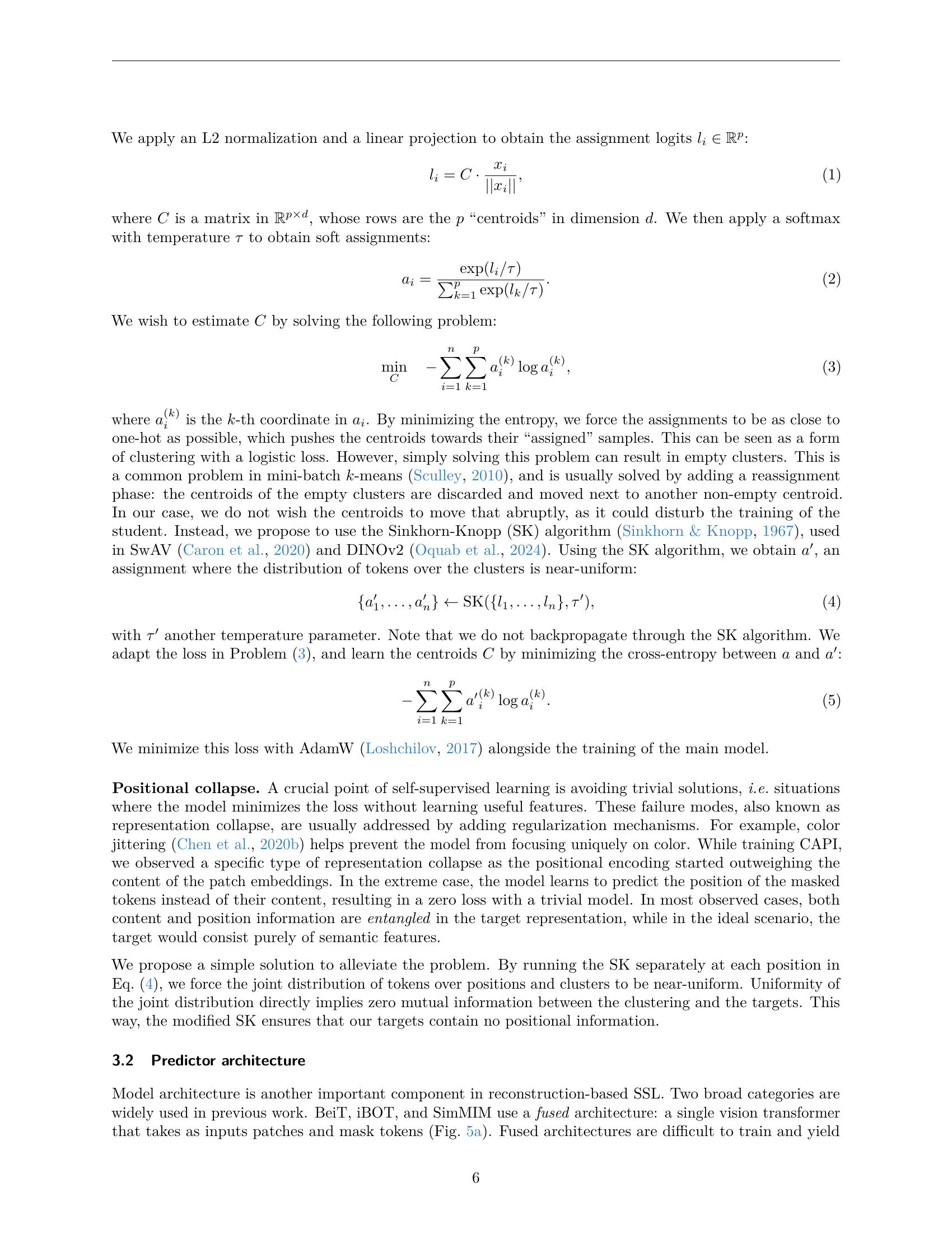
Clustering Loss
#

The concept of a clustering loss function in the context of self-supervised learning is intriguing. It leverages the idea of grouping similar image patches into clusters as a form of representation learning, moving beyond pixel-level reconstruction. Instead of directly predicting pixel values, the model learns to predict the cluster assignment of masked patches. This approach offers several advantages. First, it’s more robust to noise and variations in the input images, as it focuses on higher-level semantic representations. Second, it can be more efficient to train since the target space (cluster assignments) is generally smaller and simpler than the pixel space. Third, this clustering loss can improve the generalizability of the learned representations, as it encourages the model to learn more abstract and invariant features. However, a careful design of the clustering algorithm and its integration into the overall training process is crucial. The choice of clustering method (e.g., k-means, online clustering) and its impact on training stability and performance needs to be carefully considered. Moreover, the design of the loss function itself, such as the temperature parameter in the softmax function, plays a critical role in balancing the trade-off between accuracy and diversity. Overall, the exploration of clustering loss functions presents a promising avenue for advancing self-supervised visual representation learning.

Ablation Studies
#

The Ablation Studies section is crucial for understanding the contribution of individual components within a proposed model. It systematically investigates the impact of each design choice by removing or altering one element at a time, while keeping others constant. This controlled experimentation helps determine which parts are essential for achieving good performance and which may be superfluous or even detrimental. In the context of a masked image modeling (MIM) system, such a study might explore different predictor architectures (e.g., comparing fused, self-attention, or cross-attention designs), investigating the effects of various masking strategies (random, blockwise, etc.), evaluating alternative loss functions, analyzing the impact of different hyperparameter settings, or assessing the influence of components like positional encodings and registers. By isolating the effects of each component, ablation studies provide strong evidence supporting the design choices in the final model. The results typically demonstrate the relative importance of each component, justifying the final architecture and hyperparameter selection. They also help in identifying potential areas for future improvement, suggesting directions for further research and model optimization. For example, if removing positional encoding drastically hurts performance, it indicates the encoding’s crucial role and highlights the need for more robust positional embedding techniques in future iterations. Ultimately, a well-executed ablation study greatly enhances the credibility and robustness of the proposed method by providing a comprehensive understanding of its strengths and weaknesses.

Future of MIM
#

The future of masked image modeling (MIM) hinges on addressing its current limitations and exploring new avenues. Improving the efficiency and scalability of MIM models is crucial, potentially through architectural innovations or more efficient training strategies. Current methods often struggle with positional collapse and instability during training. Developing robust loss functions and regularization techniques to mitigate these issues is essential. The exploration of different masking strategies beyond random or block masking, perhaps incorporating more sophisticated approaches based on objectness or saliency, could improve performance. Combining MIM with other self-supervised learning approaches like contrastive learning or clustering could potentially boost performance and create a more versatile model. Finally, applying MIM to new and diverse data modalities, such as videos or 3D point clouds, will expand MIM’s applicability and lead to even more advanced representations. Addressing these key areas will unlock the full potential of MIM, leading to further breakthroughs in self-supervised visual representation learning.

More visual insights
#

More on figures

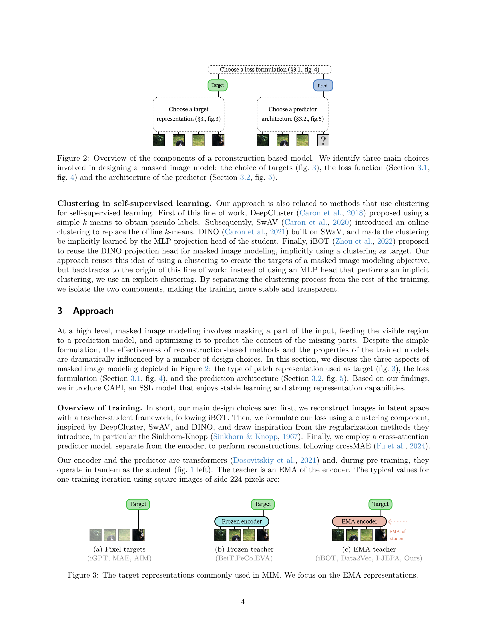
🔼 Figure 2 illustrates the key design choices in building a masked image modeling (MIM) system. The diagram highlights that three major decisions shape the effectiveness of a reconstruction-based MIM model: First, selecting the target representation used during training (further detailed in Figure 3). Second, choosing the appropriate loss function to optimize the model (explained in Section 3.1 and Figure 4). Third, defining the architecture of the predictor network responsible for reconstructing the masked image regions (discussed in Section 3.2 and Figure 5).
read the caption
Figure 2: Overview of the components of a reconstruction-based model. We identify three main choices involved in designing a masked image model: the choice of targets (fig. 3), the loss function (Section 3.1, fig. 4) and the architecture of the predictor (Section 3.2, fig. 5).

🔼 This figure illustrates different target representations used in masked image modeling (MIM). Specifically, it highlights the use of pixel-level targets, a common approach in early MIM methods like iGPT, MAE, and AIM. In these methods, the model is trained to directly reconstruct the masked pixel values, making the target representation identical to the raw pixel data.
read the caption
(a) Pixel targets (iGPT, MAE, AIM)

🔼 This figure shows different target representations used in Masked Image Modeling (MIM). Specifically, it highlights the approach where a frozen teacher network provides the target representation for the student network to learn from. The teacher network’s weights are fixed, and its output is used as the target for the MIM task. This contrasts with methods that use an online teacher (EMA) or pixel targets for training.
read the caption
(b) Frozen teacher (BeiT,PeCo,EVA)

🔼 This figure shows the different target representations used in masked image modeling (MIM). The figure illustrates three approaches to selecting the target representation during training: (a) Pixel targets, (b) Frozen teacher, and (c) EMA (exponential moving average) teacher. The EMA teacher approach, which is used in CAPI, Data2Vec, I-JEPA, and other methods, updates the teacher representation using an exponential moving average of the student’s representation. This method provides a more stable training signal and often leads to better results.
read the caption
(c) EMA teacher (iBOT, Data2Vec, I-JEPA, Ours)

🔼 This figure illustrates different target representation strategies employed in Masked Image Modeling (MIM). It compares three main approaches: using pixel-level targets (as in iGPT, MAE, and AIM), using the frozen representation of a teacher network (as in BeiT, PeCo, and EVA), and using the Exponential Moving Average (EMA) of a teacher network’s representation (as in iBOT, Data2Vec, I-JEPA, and the authors’ proposed CAPI method). The figure highlights the authors’ focus on EMA-based representations, emphasizing their advantages in MIM.
read the caption
Figure 3: The target representations commonly used in MIM. We focus on the EMA representations.

🔼 This figure illustrates the direct loss function used in masked image modeling. The direct loss calculates the difference between the predicted values and target values directly, without any intermediate steps. This type of loss is used in methods like MAE and I-JEPA. The figure likely shows a visual representation of this loss calculation, perhaps illustrating the flow of gradients used during backpropagation. This direct approach contrasts with other loss formulations shown later in the paper that involve clustering or other intermediate steps before comparing predictions to targets.
read the caption
(a) Direct loss (MAE, I-JEPA)

🔼 This figure illustrates the DINO loss function, used in masked image modeling methods such as iBOT and DINOv2. The DINO loss leverages a teacher-student framework. The teacher network produces embeddings that are used as targets. The student network tries to predict these targets. The loss function measures the discrepancy between student predictions and teacher-produced embeddings. The EMA (Exponential Moving Average) of the teacher’s output is used in this process for stability and to improve the learned features.
read the caption
(b) DINO loss (iBOT, DINOv2)

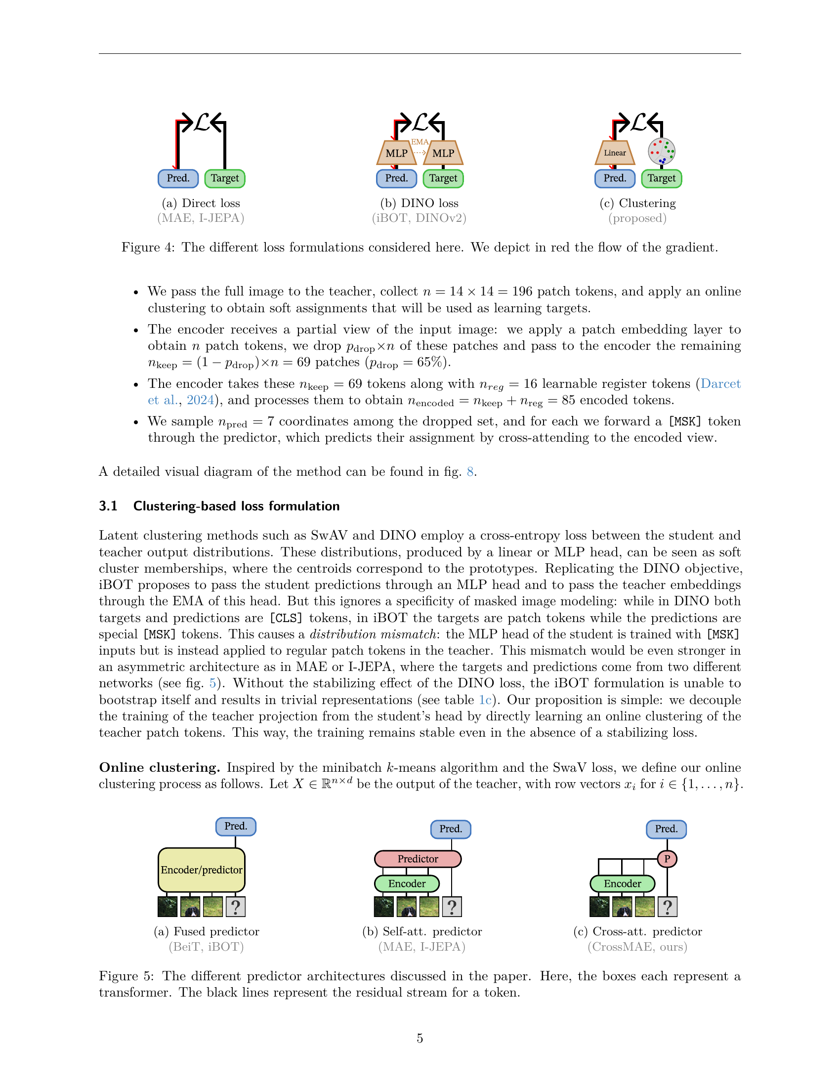
🔼 This figure illustrates the clustering-based loss function proposed by the authors. Unlike previous methods that rely on cross-entropy between student and teacher output distributions (often using an MLP head), this approach directly uses soft cluster assignments (obtained via online clustering of teacher embeddings) as the target signal. The gradient flow is depicted in red, highlighting that the loss is solely focused on predicting the correct cluster assignment for masked image patches and not reliant on any additional objectives such as contrastive loss or reconstruction loss. This design choice improves stability during training, a key improvement over prior methods.
read the caption
(c) Clustering (proposed)

🔼 This figure compares three different loss formulations used in masked image modeling. The ‘Direct loss’ directly computes the loss between the predicted and target representations. The ‘DINO loss’ uses a cross-entropy loss between the student and teacher’s output distributions, which are considered as soft cluster memberships. The ‘Clustering’ approach employs a clustering-based loss that leverages the prediction of latent clusterings. The red arrows in the diagram illustrate the gradient flow for each method.
read the caption
Figure 4: The different loss formulations considered here. We depict in red the flow of the gradient.

🔼 This figure illustrates the ‘fused predictor’ architecture used in some masked image modeling methods. In this design, a single transformer processes both the visible image patches and the special mask tokens representing missing regions. The model directly predicts pixel values or latent representations from this fused input. This is in contrast to other designs where a separate predictor processes only the mask tokens, or where reconstruction occurs in a different feature space. The examples cited here, BeiT and iBOT, demonstrate this architectural approach.
read the caption
(a) Fused predictor (BeiT, iBOT)

🔼 This figure shows a self-attention predictor architecture used in masked image modeling. The architecture consists of an encoder and a predictor, both implemented as transformers. Unlike a fused architecture (where encoding and prediction happen in a single transformer), this split architecture separates the encoding of visible image patches from the prediction of masked patches. The predictor uses self-attention to focus on the encoded features of the visible patches to predict the content of the missing ones. This approach differs from other architectures like fused predictors which process both visible and masked tokens in one transformer or cross-attention based predictors which use cross-attention to combine the masked tokens with other context.
read the caption
(b) Self-att. predictor (MAE, I-JEPA)

🔼 This figure illustrates the cross-attention predictor architecture used in the CAPI model. Unlike fused or self-attention predictor architectures, the cross-attention predictor maintains separate encoder and predictor components. The encoder processes the visible image patches, while the predictor, using cross-attention, predicts the features of the masked patches based on the encoder’s output. This design enhances efficiency and stability, as each prediction is independent of other positions, avoiding the need for repeated predictor passes. This architecture is inspired by CrossMAE and distinguishes CAPI from other masked image modeling methods.
read the caption
(c) Cross-att. predictor (CrossMAE, ours)

🔼 Figure 5 illustrates three different architectures for the predictor component in a masked image modeling system. Each architecture uses transformers, represented by boxes. The black lines show the residual connections (the path a token takes) between the different transformer layers within each architecture. The three architectures are: (a) A fused predictor, where the encoder and predictor are a single transformer; (b) A self-attention predictor where the encoder and the predictor are separate transformers and the predictor utilizes self-attention; and (c) A cross-attention predictor, also with separate encoder and predictor transformers, where the predictor uses cross-attention to access information from the encoder.
read the caption
Figure 5: The different predictor architectures discussed in the paper. Here, the boxes each represent a transformer. The black lines represent the residual stream for a token.

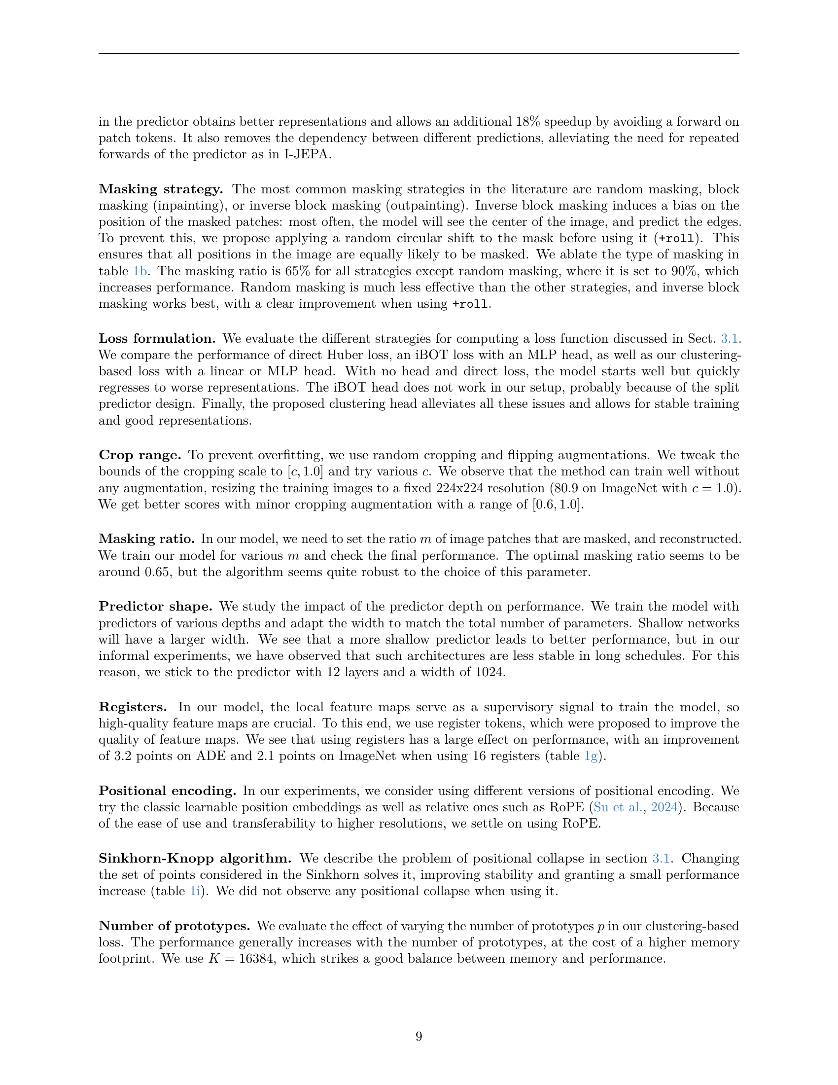
🔼 Figure 6 presents the results of ablation studies examining the impact of various parameters on the model’s performance. The left panel shows how the number of prototypes used in the clustering-based loss function affects the model’s performance on ImageNet and ADE20K. The center panel illustrates the model’s performance as a function of training duration. The right panel compares model performance when trained on different datasets: ImageNet-1k, ImageNet-22k, and LVD-142M.
read the caption
Figure 6: Additional ablation experiments. (Left) Influence of the number of prototypes. (center) Influence of the training length. Each point here is an independent training. (right) Influence of the training dataset.

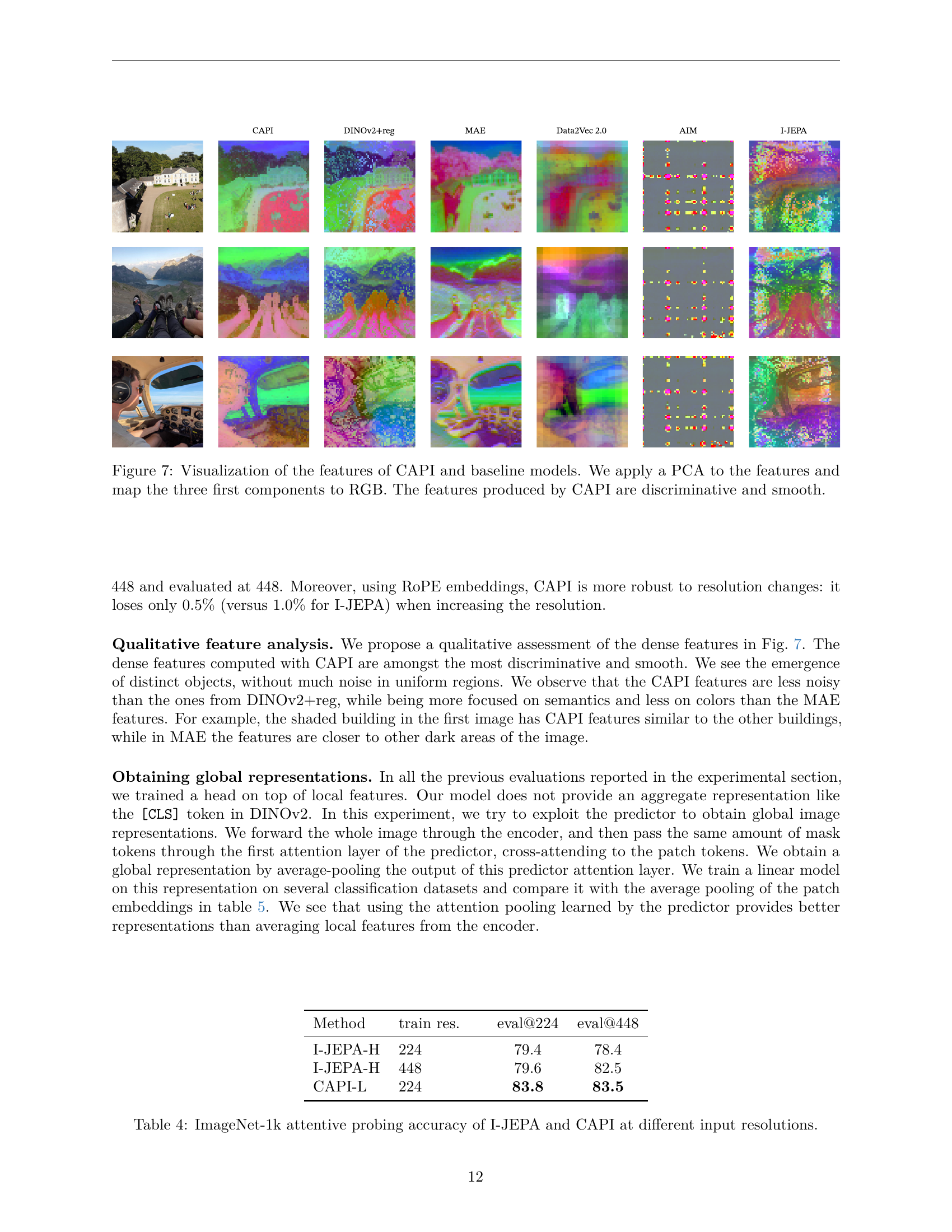
🔼 This figure visualizes the features learned by the CAPI model and several baseline models. Principal Component Analysis (PCA) was used to reduce the dimensionality of the feature maps to three principal components, which were then mapped to the red, green, and blue channels of an RGB image. The resulting images provide a visual representation of the learned features. The caption highlights that the features produced by CAPI are distinctly different and smoother compared to the baseline models, suggesting superior quality and potentially better performance.
read the caption
Figure 7: Visualization of the features of CAPI and baseline models. We apply a PCA to the features and map the three first components to RGB. The features produced by CAPI are discriminative and smooth.

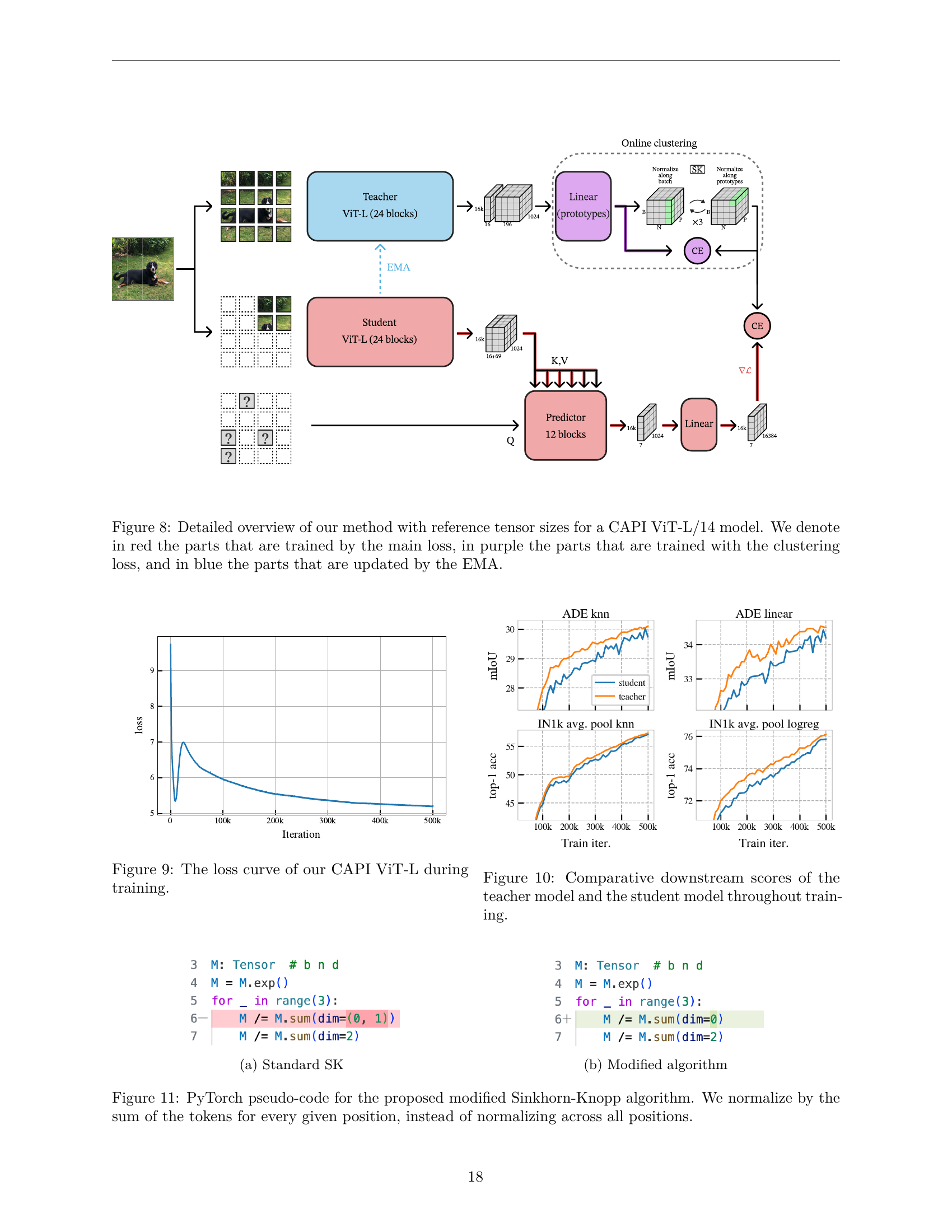
🔼 Figure 8 provides a detailed visualization of the CAPI model architecture, highlighting the flow of data and the different training mechanisms. The diagram shows the teacher and student networks (both ViT-L/14), emphasizing the role of the exponential moving average (EMA) in updating the teacher. It also illustrates the clustering process used to generate the training signal (soft assignments) for the student, which predicts the missing image patches. The color-coding helps distinguish components trained by the main loss (red), the clustering loss (purple), and the EMA updates (blue). Tensor sizes are included for a better understanding of the model’s dimensions.
read the caption
Figure 8: Detailed overview of our method with reference tensor sizes for a CAPI ViT-L/14 model. We denote in red the parts that are trained by the main loss, in purple the parts that are trained with the clustering loss, and in blue the parts that are updated by the EMA.

🔼 This figure shows the training loss curve for the CAPI ViT-L model. The x-axis represents the training iteration, and the y-axis represents the loss value. The curve demonstrates a smooth downward trend, indicating stable training and the absence of plateaus or significant instability.
read the caption
Figure 9: The loss curve of our CAPI ViT-L during training.

🔼 This figure displays the performance of both the teacher and student models throughout the training process. The x-axis represents the training iteration, while the y-axis shows the accuracy. Two sets of curves are presented: top-1 accuracy on ImageNet and mIoU scores on ADE20K, both for the teacher and student models. The purpose is to demonstrate the effectiveness of self-distillation, where the more advanced teacher model guides the student’s learning, and to show the stability and improvement over time.
read the caption
Figure 10: Comparative downstream scores of the teacher model and the student model throughout training.

🔼 This figure shows the pseudo-code for the standard Sinkhorn-Knopp algorithm. It details the iterative normalization process used to obtain a near-uniform distribution of tokens over clusters. The algorithm takes a tensor M as input and iteratively normalizes it along rows and columns. The normalization is done by dividing each element by the sum of elements in its row and then by the sum of elements in its column. This process is repeated until convergence, producing the output tensor M.
read the caption
(a) Standard SK

🔼 This figure presents the pseudo-code for a modified Sinkhorn-Knopp algorithm. The original algorithm (shown in (a)) and the modification are compared. The modification involves normalizing by the sum of tokens for every position rather than normalizing across all positions, which addresses positional collapse in masked image modeling.
read the caption
(b) Modified algorithm

🔼 This figure presents the PyTorch pseudo-code for the modified Sinkhorn-Knopp algorithm used in the paper. The Sinkhorn-Knopp algorithm is an iterative procedure to find a doubly stochastic matrix. This modification involves normalizing the sum of tokens for each position instead of normalizing across all positions in each iteration, leading to a more stable and efficient computation for the online clustering task. This approach enhances the clustering process and contributes to the overall improved performance of the masked image modeling technique.
read the caption
Figure 11: PyTorch pseudo-code for the proposed modified Sinkhorn-Knopp algorithm. We normalize by the sum of the tokens for every given position, instead of normalizing across all positions.

🔼 This figure visualizes the feature maps generated by various self-supervised vision models, including CAPI, DINOv2+reg, BEiT, AIM, MAE, I-JEPA, and data2vec2, each with different model sizes and resolutions. PCA (Principal Component Analysis) is used to reduce the dimensionality of the dense feature maps for each image. The top three principal components are then mapped to the red, green, and blue channels of the RGB color space, allowing for visual comparison of the feature representations. This provides insights into how different models capture and represent visual information.
read the caption
Figure 12: Visualization of the features produced by CAPI and other vision models at various resolutions: CAPI ViT-L/14, DINOv2+reg ViT-g/14 (Darcet et al., 2024), BEiT ViT-L/16 (Bao et al., 2021), AIM ViT-3B/14 (El-Nouby et al., 2024), MAE ViT-H/14 (El-Nouby et al., 2024), I-JEPA ViT-H/14 (Assran et al., 2023), and data2vec2 ViT-L/16 (Baevski et al., 2022). We apply a PCA decomposition to the dense outputs produced by each model for each image individually, and rescale the three first components to the RGB range for visualization.

🔼 This figure visualizes the features produced by the CAPI ViT-L/14 model applied to images at 560 pixel resolution. A Principal Component Analysis (PCA) is performed on the dense feature outputs, and the results are displayed. The first column shows the top three principal components mapped to RGB. The remaining columns depict the first eight channels of the PCA, each visualized individually using a coolwarm colormap.
read the caption
Input

🔼 This figure visualizes the features produced by the CAPI ViT-L/14 model applied to images at 560 pixel resolution. A principal component analysis (PCA) is performed on the dense feature outputs from the model across all images. The first column displays the top three principal components mapped to RGB colors. The subsequent eight columns show the first eight individual channels using a coolwarm colormap. This provides a visual representation of the learned features, highlighting their spatial organization and potential discriminative qualities.
read the caption
PCA

🔼 This figure visualizes the features produced by the CAPI ViT-L/14 model applied to images at 560 pixel resolution. A principal component analysis (PCA) is performed on the dense feature outputs. The first column shows the first three principal components mapped to RGB channels, offering a visual representation of the main feature variations. The subsequent eight columns display channels 0 through 7 individually, using a coolwarm colormap for better visualization of feature intensity and distribution. This visualization helps in understanding the nature and distribution of learned features within the CAPI model.
read the caption
Channel 0

🔼 This figure visualizes the features produced by the CAPI ViT-L/14 model applied to images at 560 pixel resolution. A Principal Component Analysis (PCA) was performed on the dense feature outputs, resulting in a dimensionality reduction. The first column displays the first three principal components mapped to RGB colors for visualization. The subsequent eight columns showcase the next eight channels of the PCA individually, using a coolwarm colormap (from Matplotlib). This visualization helps to understand the nature of the learned features, demonstrating the model’s ability to capture different aspects of the images.
read the caption
Channel 1

🔼 This figure visualizes the features extracted from the CAPI ViT-L/14 model applied to images at 560 pixel resolution. It shows the second principal component (Channel 2) resulting from a Principal Component Analysis (PCA) of the features. The image showcases the features’ spatial distribution and how they capture different aspects of the image content. The visualization helps understand how well the model’s features can discriminate and capture relevant semantic information from the image.
read the caption
Channel 2

🔼 This figure visualizes the features produced by the CAPI ViT-L/14 model applied to images at 560 pixel resolution. A Principal Component Analysis (PCA) is performed on the dense feature outputs across all images. The visualization shows the principal components of the features as RGB and the first eight channels individually using a colormap.
read the caption
Channel 3

🔼 This figure visualizes the features produced by the CAPI ViT-L/14 model applied to images at 560 pixel resolution. A Principal Component Analysis (PCA) is performed on the dense feature outputs. The first column shows the first three principal components mapped to RGB values. The remaining eight columns display the first eight channels of the features individually, using a coolwarm colormap.
read the caption
Channel 4

🔼 This figure visualizes the features produced by the CAPI ViT-L/14 model applied to images at 560 pixel resolution. It shows the features using Principal Component Analysis (PCA). The first column displays the first three principal components mapped to RGB colors. The subsequent columns display channels 0 through 7 individually using a coolwarm colormap.
read the caption
Channel 5

🔼 This figure visualizes the features extracted by the CAPI ViT-L/14 model applied to images at 560 pixel resolution. A Principal Component Analysis (PCA) is performed on the dense feature outputs from the model, and the visualization shows the first eight principal components individually. Each component is represented using a coolwarm colormap, providing a visual representation of the model’s learned features across various image regions.
read the caption
Channel 6

🔼 This figure visualizes the features produced by the CAPI ViT-L/14 model applied to images at 560 pixel resolution. It uses Principal Component Analysis (PCA) to reduce the dimensionality of the features, then displays the results. The first column shows the top three principal components mapped to the RGB color space. The subsequent eight columns show channels 0 through 7 individually, using a coolwarm colormap.
read the caption
Channel 7

🔼 This figure visualizes the features extracted by the CAPI ViT-L/14 model when processing images at a resolution of 560 pixels. A principal component analysis (PCA) was performed on the model’s dense output across multiple images to reduce dimensionality. The resulting principal components are then displayed. The first column shows the first three principal components mapped to the red, green, and blue color channels (RGB), providing a visual representation of the most significant variations in the data. The following eight columns represent the next eight principal components, visualized individually using a ‘coolwarm’ colormap from the Matplotlib library, showcasing additional feature variations in the dataset.
read the caption
Figure 13: Visualization of the features produced by CAPI ViT-L/14 applied to images at 560 pixel resolution. We apply a PCA decomposition to the dense outputs produced by the model across all images. The first column shows the first 3 components as RGB. The next eight columns show the first eight channels individually using a coolwarm colormap from Matplotlib (Hunter, 2007).

More on tables

	ADE	IN1k
Fused	23.8	73.1
Split, self-attn	27.9	77.7
Split, cross-attn	29.1	81.4

🔼 This table presents an ablation study on different masking strategies used in masked image modeling. It compares the performance of various masking techniques, including random masking, block masking, inverse block masking with and without a random circular shift, on both ImageNet-1k classification and ADE20K segmentation tasks. The results demonstrate the impact of the masking strategy on model performance and highlight the effectiveness of inverse block masking with a circular shift in improving representation learning.
read the caption
(b) Masking strategy

	ADE	IN1k
random	23.6	76.4
block	25.6	79.9
inv. block	27.2	80.7
inv. block +roll	29.1	81.4

🔼 This table presents an ablation study comparing different loss functions used in the masked image modeling (MIM) process. It shows the impact of using different loss functions on the model’s performance in terms of both ImageNet-1k classification accuracy and ADE20K segmentation mIoU. The table allows researchers to compare the results of direct loss, DINO loss, and the proposed clustering-based loss. It helps to understand the effect of different loss formulations on the model’s performance and stability during training.
read the caption
(c) Loss formulation

head	loss	ADE	IN1k
$\varnothing$	I-JEPA	23.7	79.3
MLP	iBOT	1.7	11.1
MLP	CAPI	26.4	80.8
Linear	CAPI	29.1	81.4

🔼 This table presents ablation study results focusing on the impact of the cropping range used during data augmentation on the performance of the CAPI model. The cropping range determines the proportion of the original image that is randomly cropped before being fed to the model during training. The table shows how different crop ranges affect performance on the ADE20K semantic segmentation and ImageNet-1k classification tasks, using a k-NN and linear probe, respectively.
read the caption
(d) Crop range

	ADE	IN1k
$[0.2,1.0]$	27.9	81.4
$[0.6,1.0]$	29.1	81.4
$[1.0,1.0]$	28.9	80.9

🔼 This table presents the ablation study on different masking ratios used in the CAPI model. The masking ratio refers to the proportion of image patches that are masked during training. The table shows how the model’s performance varies (measured by ADE20K and ImageNet1k scores) when different ratios of patches are masked out.
read the caption
(e) Masking ratio

	ADE	IN1k
55%	28.0	81.1
65%	29.1	81.4
75%	28.1	81.2

🔼 This table presents ablation studies on the predictor’s architecture. Different depths and widths of the predictor are explored, while keeping the total number of parameters constant. The results show the impact of these architectural choices on both ImageNet-1k classification accuracy and ADE20K semantic segmentation mIoU.
read the caption
(f) Predictor shape

depth	width	ADE	IN1k
5	1536	30.9	81.5
12	1024	29.1	81.4
21	768	28.3	81.3

🔼 This table presents ablation study results focusing on the impact of the number of register tokens used in the model. Register tokens are additional tokens added to the input sequence during training to improve the quality of learned feature maps. The table shows how the number of register tokens affects the performance on the ADE20K segmentation and ImageNet-1k classification tasks, comparing the results with different numbers of register tokens (0, 16). It demonstrates the performance gain achieved by including registers and the optimal number leading to best performance.
read the caption
(g) Number of registers

	ADE	IN1k
0	25.9	79.3
16	29.1	81.4

🔼 This table presents ablation study results focusing on the positional encoding method used in the masked image modeling (MIM) process. It compares the performance of the model trained using the standard positional encoding against a model using a proposed alternative. The results show the impact of this design choice on both ImageNet-1k classification accuracy and ADE20K segmentation mIoU. The ‘Proposed’ method appears to improve performance slightly but within a small margin.
read the caption
(h) Positional encoding

	ADE	IN1k
learnable	30.0	81.6
RoPE	29.1	81.4

🔼 Table 1(i) shows the ablation study on the effect of using the Sinkhorn-Knopp algorithm in the online clustering process. It compares the performance of using the standard Sinkhorn-Knopp algorithm against a proposed modification where the algorithm is run separately at each position to prevent positional collapse, a common issue in self-supervised learning. The table reports the performance in terms of ADE20K segmentation mIoU and ImageNet-1k classification accuracy.
read the caption
(i) Sinkhorn-Knopp algorithm

	ADE	IN1k
Standard	28.5	81.3
Proposed	29.1	81.4

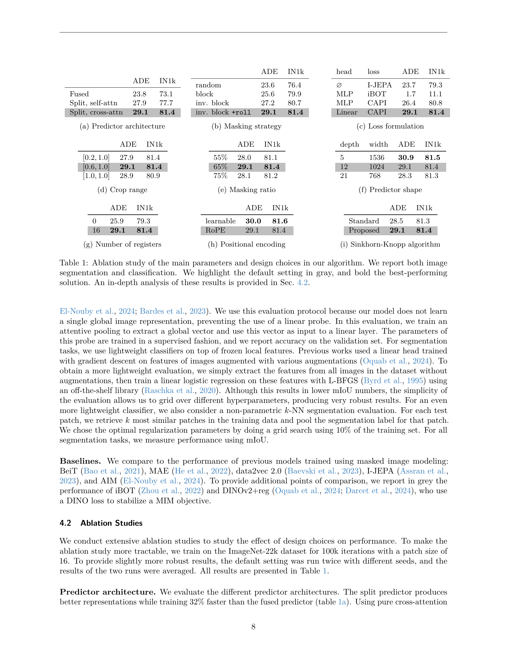
🔼 This ablation study investigates the impact of various design choices within the CAPI model on both image classification and segmentation tasks. The table systematically varies parameters such as predictor architecture, masking strategy, loss function, and hyperparameters, showing the effect on ImageNet-1k classification accuracy and ADE20k segmentation mIoU. The default configuration is highlighted in gray, and the best-performing settings are bolded. A detailed analysis of these results can be found in section 4.2 of the paper.
read the caption
Table 1: Ablation study of the main parameters and design choices in our algorithm. We report both image segmentation and classification. We highlight the default setting in gray, and bold the best-performing solution. An in-depth analysis of these results is provided in Sec. 4.2.

#prototypes	ADE	IN1k
1024	14.9	73.8
2048	19.8	77.4
4096	27.5	80.7
8192	28.5	81.3
16384	29.1	81.4
32768	29.1	81.7

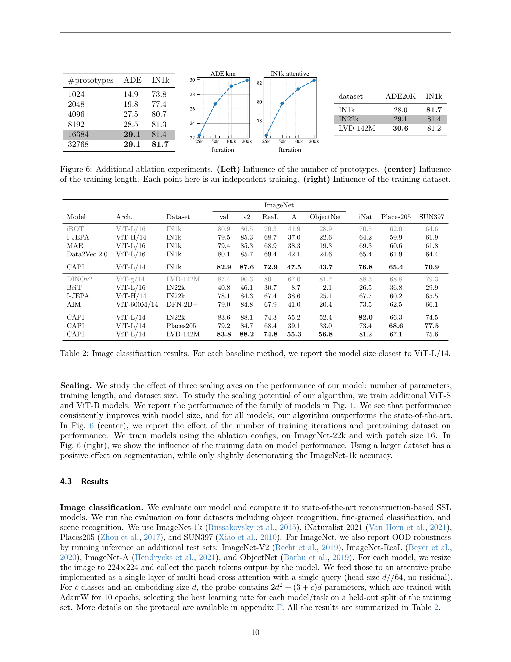
🔼 This table presents the image classification results for various self-supervised learning models. It compares the performance of the proposed CAPI model against several established baselines on various image classification datasets. The performance is measured using accuracy on different datasets. For a fair comparison, the table focuses on baselines that have model sizes similar to that of the CAPI model (ViT-L/14). The datasets used include ImageNet, ObjectNet, iNaturalist, Places205, and SUN397. The table allows for a quantitative evaluation of CAPI’s effectiveness in learning generalizable visual representations compared to other state-of-the-art methods.
read the caption
Table 2: Image classification results. For each baseline method, we report the model size closest to ViT-L/14.

dataset	ADE20K	IN1k
IN1k	28.0	81.7
IN22k	29.1	81.4
LVD-142M	30.6	81.2

🔼 Table 3 presents a comparison of CAPI’s performance against state-of-the-art models on image segmentation using only frozen features (no further training of the model). Both k-NN and linear methods are used for segmentation and the results (mIoU scores) are presented for various datasets (ADE20k, Pascal VOC, Cityscapes). Additionally, results from non-MIM (Masked Image Modeling) self-supervised learning models are included as a benchmark to highlight CAPI’s competitive performance, achieved using only a MIM approach.
read the caption
Table 3: Comparison with the state of the art on image segmentation using frozen features. We report both k𝑘kitalic_k-NN and linear segmentation performance. For reference, we also report the performance of some other non-MIM SSL models. This shows that CAPI narrows the gap using only a MIM approach.

Method	train res.	eval@224	eval@448
I-JEPA-H	224	79.4	78.4
I-JEPA-H	448	79.6	82.5
CAPI-L	224	83.8	83.5

🔼 This table presents a comparison of the ImageNet-1k attentive probing accuracy achieved by the I-JEPA and CAPI models when using different input resolutions (224x224 and 448x448 pixels). It demonstrates the performance of each model at various input sizes, showing the robustness or sensitivity of their respective architectures to changes in image resolution.
read the caption
Table 4: ImageNet-1k attentive probing accuracy of I-JEPA and CAPI at different input resolutions.

	IN1k		iNat21	SUN397
Representation	$k$ -NN	Linear	Linear	Linear
avg. pooling	57.1	77.1	49.1	73.3
predictor pooling	73.8	81.1	69.6	77.4

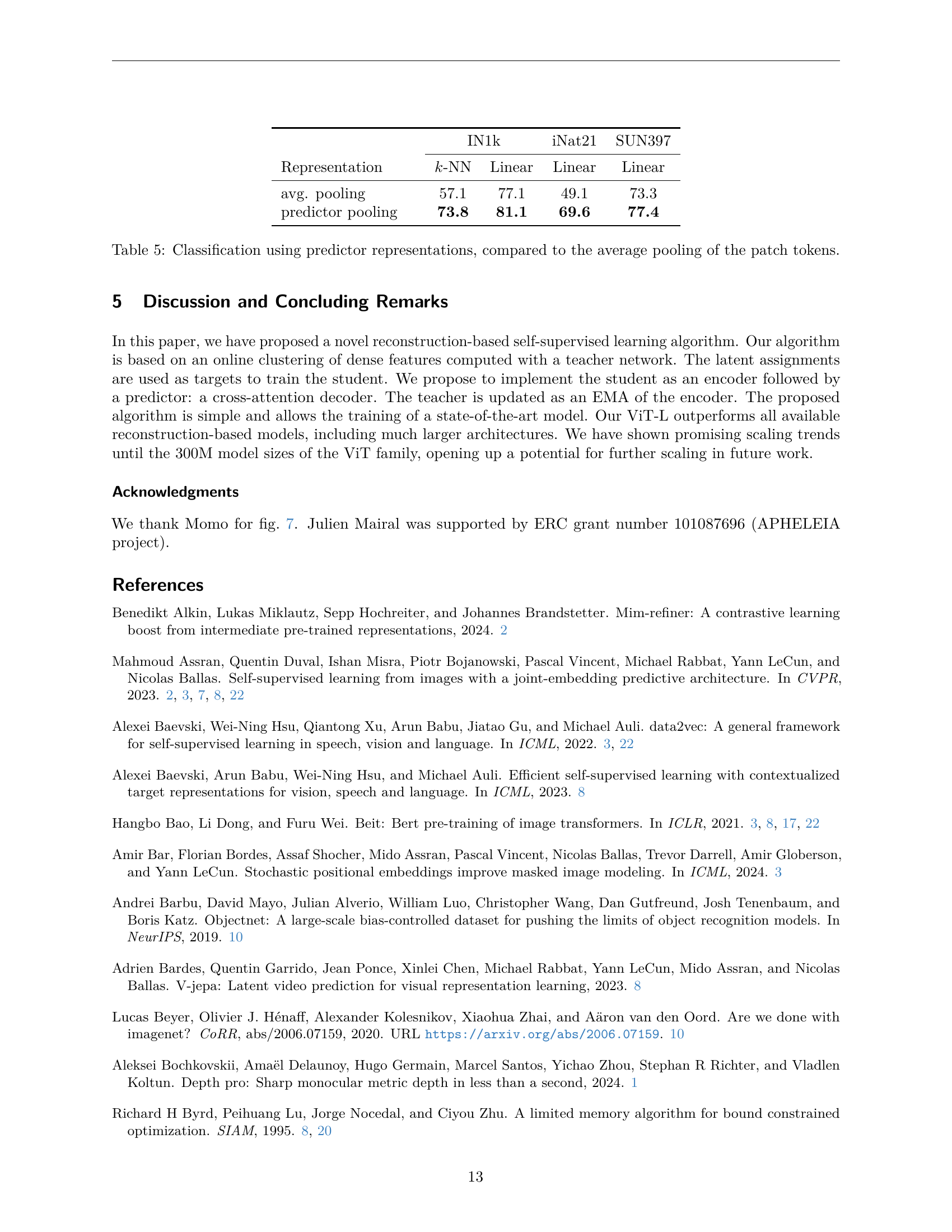
🔼 This table compares the performance of two different methods for obtaining image representations from a vision transformer model: average pooling and predictor pooling. Average pooling calculates the average of the patch tokens, while predictor pooling uses a learned predictor to generate a more informative representation. The table shows the classification accuracy achieved using these two types of representations on three different datasets: ImageNet-1k, iNaturalist 2021, and SUN397. Both k-NN and linear classifiers were used for evaluation.
read the caption
Table 5: Classification using predictor representations, compared to the average pooling of the patch tokens.

Hyperparameter	Value
Batch size	16384
Optimizer	AdamW
Learning rate	1e-3
Teacher momentum	$1-lr$
Clustering lr	$\frac{1}{2}lr$
lr schedule	linear warmup + trunc. cosine
Warmup length	10%
cosine truncation	20%
Weight decay	0.1
AdamW $\beta$	(0.9, 0.95)
Number of prototypes	16384
Student temperature	0.12
Teacher temperature	0.06
Num SK iter	3
Stochastic depth	0.2
Weight init	xavier_uniform
Norm layer	RMSnorm
Norm $\varepsilon$	1e-5
Patch embed lr	$0.2\cdot{}$ lr
Norm layer wd	$0.1\cdot{}$ wd
Image size	224
Augmentations	RRCrop, HFlip
Training dtype	bf16
Parallelism	FSDP
Pred. / im	7
Layerscale	No
Biases	No
Rope frequencies	logspace(7e-4, 7), axial
Masking type	inverse block+roll
Masking ratio	65%

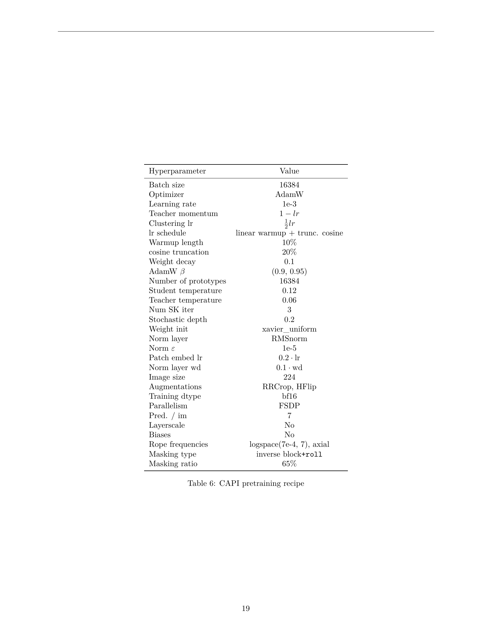
🔼 This table details the hyperparameters used for pre-training the CAPI model. It lists various settings, including batch size, optimizer, learning rate, weight decay, number of prototypes, temperature parameters, and more, providing a comprehensive overview of the training configuration.
read the caption
Table 6: CAPI pretraining recipe

		knn			logreg
model	standardization	ADE	Cityscapes	VOC2012	ADE	Cityscapes	VOC2012
CAPI	False	32.5	39.2	64.9	37.9	44.7	73.2
CAPI	True	33.0	39.2	65.2	37.7	44.3	73.3
aim 600M	False	14.3	27.8	38.5	7.1	28.3	61.3
aim 600M	True	nan	32.1	60.2	31.5	38.2	67.0
dinov2 vitg14+reg	False	33.8	42.0	63.1	38.9	46.8	72.9
dinov2 vitg14+reg	True	34.0	42.0	63.0	39.0	46.8	72.8
ijepa vith14 in1k	False	20.1	25.9	57.4	25.2	33.5	63.0
ijepa vith14 in1k	True	20.8	26.4	56.7	25.7	34.5	63.6
ijepa vith14 in22k	False	17.9	22.9	56.2	24.1	32.8	63.6
ijepa vith14 in22k	True	18.9	23.2	55.0	26.4	34.2	64.2
mae vitl16	False	7.8	25.3	17.3	27.4	38.4	61.5
mae vitl16	True	21.5	32.8	53.7	27.4	38.5	61.5

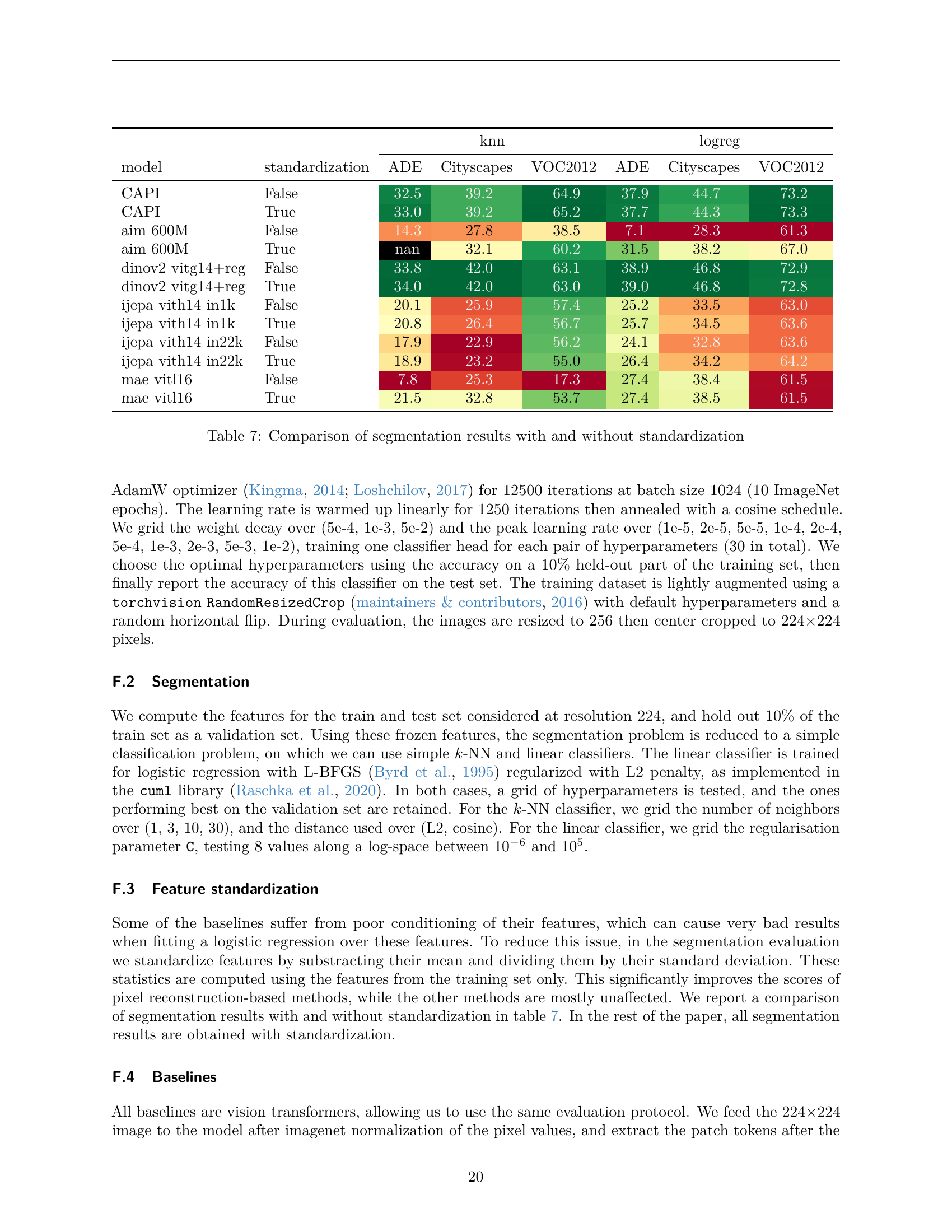
🔼 This table compares the performance of various masked image modeling methods on three semantic segmentation datasets: ADE20K, Pascal VOC 2012, and Cityscapes. The comparison is made with and without feature standardization (a preprocessing step to normalize the features). The table shows the mean Intersection over Union (mIoU) scores obtained using both k-NN and linear classifiers, providing a comprehensive assessment of how standardization affects performance across different models and datasets.
read the caption
Table 7: Comparison of segmentation results with and without standardization

uid

dataset

#iter

patch size

enc depth

pred depth

enc dim

pred dim

mom.

clust. lr

masking

ratio

roll

teacher head

student head

loss

pos. enc.

#reg.

crop scale

Meb2b

LVD-142M

500k

1024

1e-03

0.999

5e-04

inv. block

65%

True

clustering

Linear

rope

modified

[60%,100%]

Mc2dd

LVD-142M

500k

768

1e-03

0.999

5e-04

inv. block

65%

True

clustering

Linear

rope

modified

[60%,100%]

M8c4d

LVD-142M

500k

384

2e-03

0.998

1e-03

inv. block

65%

True

clustering

Linear

rope

modified

[60%,100%]

Adcab

IN22k

100k

1024

2e-03

0.996

1e-03

inv. block

65%

True

clustering

Linear

rope

modified

[60%,100%]

Ae3f9

IN22k

100k

1024

2e-03

0.996

1e-03

inv. block

65%

True

clustering

Linear

rope

modified

[60%,100%]

A0dd4

IN22k

100k

1024

2e-03

0.996

1e-03

random

90%

False

clustering

Linear

rope

modified

[60%,100%]

A9b4a

IN22k

100k

1024

2e-03

0.996

1e-03

block

65%

False

clustering

Linear

rope

modified

[60%,100%]

A7cc0

IN22k

100k

1024

2e-03

0.996

1e-03

inv. block

65%

False

clustering

Linear

rope

modified

[60%,100%]

A3bb3

IN22k

100k

1024

2e-03

0.996

1e-03

inv. block

65%

True

identity

Huber

rope

standard

[60%,100%]

A2fcb

IN22k

100k

1024

2e-03

0.996

1e-03

inv. block

65%

True

EMA

MLP

rope

modified

[60%,100%]

Aeb48

IN22k

100k

1024

2e-03

0.996

1e-03

inv. block

65%

True

clustering

MLP

rope

modified

[60%,100%]

A74f9

IN22k

100k

1024

2e-03

0.996

1e-03

inv. block

65%

True

clustering

Linear

rope

modified

[100%,100%]

Ae7b3

IN22k

100k

1024

2e-03

0.996

1e-03

inv. block

65%

True

clustering

Linear

rope

modified

[20%,100%]

A41b8

IN22k

100k

1024

2e-03

0.996

1e-03

inv. block

55%

True

clustering

Linear

rope

modified

[60%,100%]

Ac8bc

IN22k

100k

1024

2e-03

0.996

1e-03

inv. block

75%

True

clustering

Linear

rope

modified

[60%,100%]

Af989

IN22k

100k

1024

1536

2e-03

0.996

1e-03

inv. block

65%

True

clustering

Linear

rope

modified

[60%,100%]

A2da0

IN22k

100k

1024

768

2e-03

0.996

1e-03

inv. block

65%

True

clustering

Linear

rope

modified

[60%,100%]

A9ce8

IN22k

100k

1024

2e-03

0.996

1e-03

inv. block

65%

True

clustering

Linear

rope

modified

[60%,100%]

A1177

IN22k

100k

1024

2e-03

0.996

1e-03

inv. block

65%

True

clustering

Linear

learn.

modified

[60%,100%]

A72fb

IN22k

100k

1024

2e-03

0.996

1e-03

inv. block

65%

True

clustering

Linear

rope

standard

[60%,100%]

M5e2e

IN22k

500k

1024

1e-03

0.999

5e-04

inv. block

65%

True

clustering

Linear

rope

modified

[60%,100%]

M2d34

IN1k

500k

1024

1e-03

0.999

5e-04

inv. block

65%

True

clustering

Linear

rope

modified

[60%,100%]

M8319

P205

500k

1024

1e-03

0.999

5e-04

inv. block

65%

True

clustering

Linear

rope

modified

[60%,100%]

Abe05

IN22k

25k

1024

2e-03

0.996

1e-03

inv. block

65%

True

clustering

Linear

rope

modified

[60%,100%]

Acd44

IN22k

50k

1024

2e-03

0.996

1e-03

inv. block

65%

True

clustering

Linear

rope

modified

[60%,100%]

A2ca8

IN22k

200k

1024

2e-03

0.996

1e-03

inv. block

65%

True

clustering

Linear

rope

modified

[60%,100%]

Aab94

IN1k

100k

1024

2e-03

0.996

1e-03

inv. block

65%

True

clustering

Linear

rope

modified

[60%,100%]

Aa428

LVD-142M

100k

1024

2e-03

0.996

1e-03

inv. block

65%

True

clustering

Linear

rope

modified

[60%,100%]

🔼 This table summarizes the different model configurations used throughout the paper. Each model is assigned a unique identifier (‘uid’). The table details key hyperparameters that varied across the experiments, offering a comprehensive overview of the experimental setup and allowing readers to easily trace model variations discussed in the results.
read the caption
Table 8: Summary of all models mentioned in the paper. We associate to each a unique uid, and detail the hyperparameters which are not constant across all runs.

Fig	Models used
fig. 1	Meb2b, Mc2dd, M8c4d
table 1(a)	Adcab, Ae3f9, Aa5a3, A7d26
table 1(b)	Adcab, Ae3f9, A0dd4, A9b4a, A7cc0
table 1(c)	Adcab, Ae3f9, A3bb3, A2fcb, Aeb48
table 1(d)	Adcab, Ae3f9, A74f9, Ae7b3
table 1(e)	Adcab, Ae3f9, A41b8, Ac8bc
table 1(f)	Adcab, Ae3f9, Af989, A2da0
table 1(g)	Adcab, Ae3f9, A9ce8
table 1(h)	Adcab, Ae3f9, A1177
table 1(i)	Adcab, Ae3f9, A72fb
section 4.3	Meb2b, M5e2e, M2d34, M8319
section 4.3	Meb2b, M5e2e, M2d34, M8319
table 4	Meb2b
fig. 7	Meb2b
table 5	Meb2b
fig. 6	Adcab, Ae3f9, Abe05, Acd44, A2ca8, Adcab, Ae3f9, Aab94, Aa428
fig. 10	Meb2b
fig. 13	Meb2b
fig. 12	Meb2b

🔼 This table provides a cross-reference between the models used throughout the paper and their appearances in various figures and tables. It’s a helpful guide for navigating the different model configurations and their corresponding results presented in the paper. Each row identifies a model by a unique alphanumeric code, then lists the figures and/or tables in which that model’s results are shown.
read the caption
Table 9: Reference of models used in different figures and tables.

TL;DR#

Key Takeaways#

Why does it matter?#

Visual Insights#

In-depth insights#

MIM Enhancements#

CAPI Framework#

Clustering Loss#

Ablation Studies#

Future of MIM#

More visual insights#

Full paper#

TL;DR
#

Key Takeaways
#

Why does it matter?
#

Visual Insights
#

In-depth insights
#

MIM Enhancements
#

CAPI Framework
#

Clustering Loss
#

Ablation Studies
#

Future of MIM
#

More visual insights
#

Full paper
#