TL;DR#
Many real-world time series forecasting problems involve multiple interconnected variables, making it challenging to apply existing pre-trained models which typically work with only single variables. Also, quantifying the uncertainty associated with predictions is crucial for making informed decisions. This research tackles these challenges.
The researchers introduce AdaPTS, a novel framework that uses adapters to transform multivariate data into a format suitable for univariate models. It uses a family of adapters, including linear and probabilistic versions. Experiments show that this approach significantly improves the accuracy of forecasts and also provides better estimates of uncertainty. The modularity of AdaPTS makes it easily adaptable to different datasets and model architectures.
Key Takeaways#
Why does it matter?#
This paper is important because it presents AdaPTS, a novel and effective framework for adapting pre-trained univariate time series foundation models to multivariate forecasting tasks. This is highly relevant given the increasing popularity of foundation models and the challenges of applying them directly to multivariate data. The framework’s modularity and scalability make it widely applicable, and its probabilistic nature allows for improved uncertainty quantification, which is crucial in real-world forecasting scenarios. Further research can explore its application to other model architectures and optimization strategies.
Visual Insights#

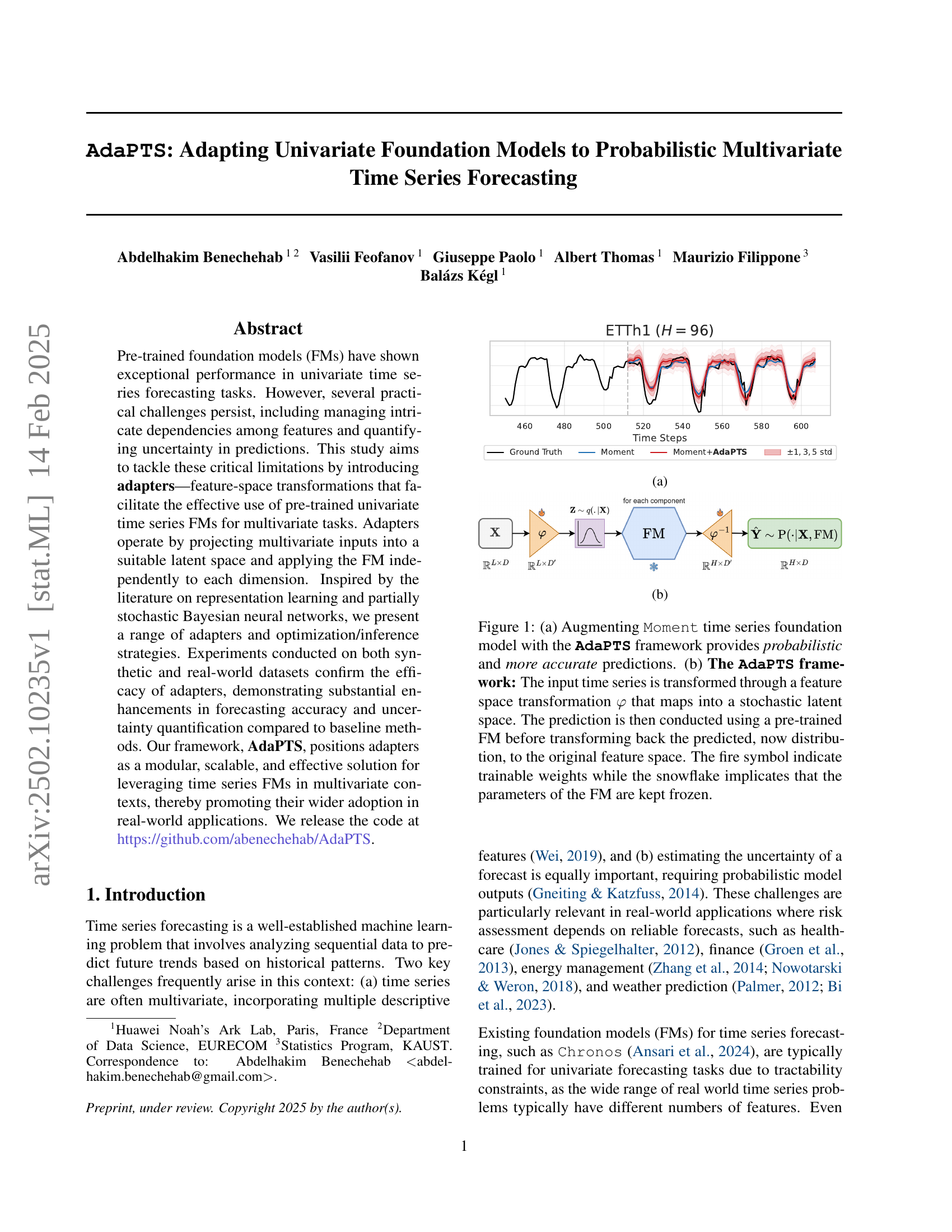
🔼 The figure shows how AdaPTS improves the accuracy of probabilistic predictions compared to ground truth. The plot displays the predictions (Moment+AdaPTS) and the ground truth for the ETTh1 dataset over time steps, clearly showing that AdaPTS improves accuracy over the Moment model alone. This is particularly evident because the prediction using AdaPTS closely follows the trends in the ground truth data.
read the caption
(a)
| Dataset | H | No adapter | with adapter | ||||
| Moment | PCA | LinearAE | dropoutLAE | LinearVAE | VAE | ||
| ETTh1 | 96 | ||||||
| 192 | |||||||
| Illness | 24 | ||||||
| 60 | |||||||
| Weather | 96 | ||||||
| 192 | |||||||
| ExchangeRate | 96 | ||||||
| 192 | |||||||
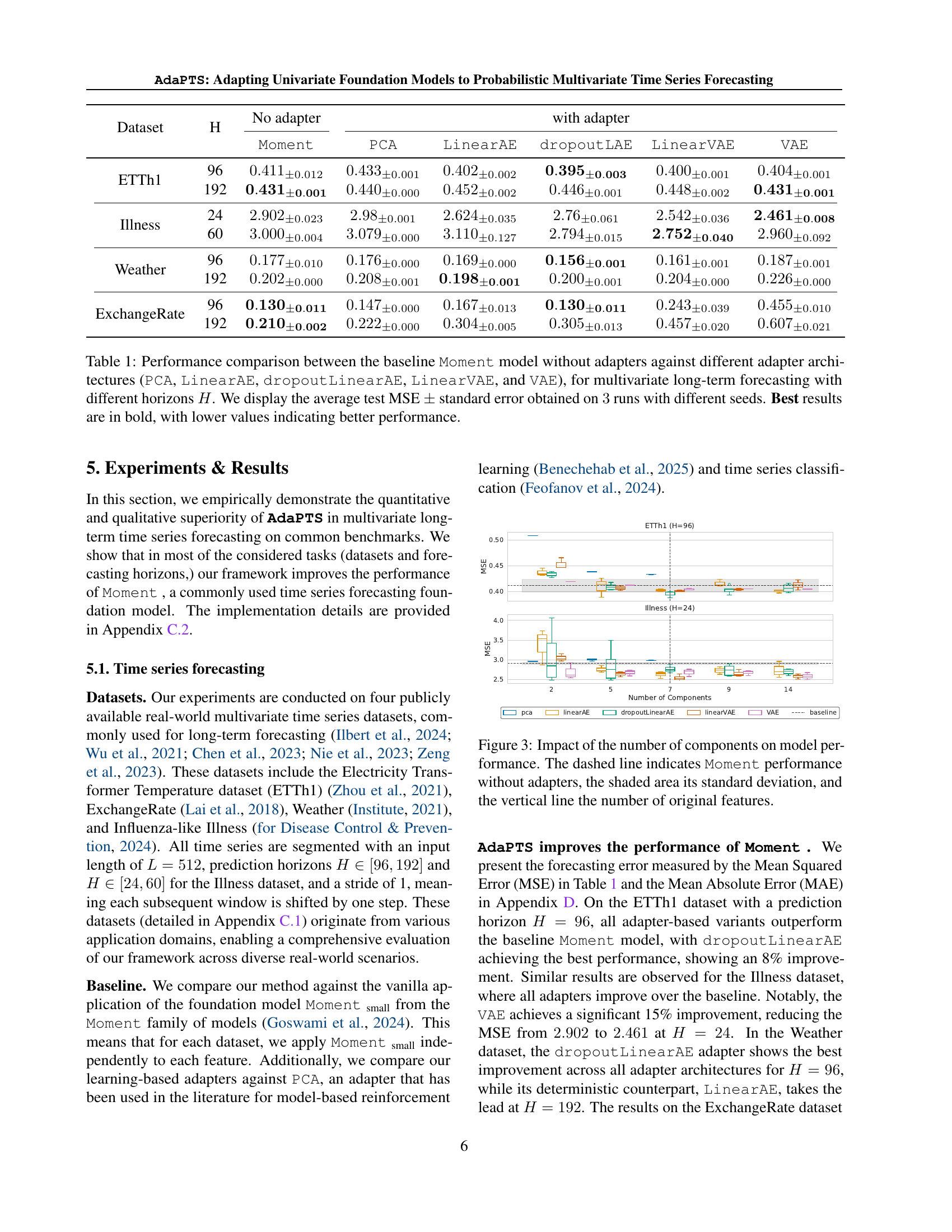
🔼 Table 1 compares the forecasting performance of the Moment model (a baseline univariate time series forecasting model) against variations of the AdaPTS framework on multiple multivariate time series datasets. AdaPTS adapts the Moment model for multivariate forecasting by incorporating several different adapter architectures: PCA (Principal Component Analysis), LinearAE (Linear AutoEncoder), dropoutLinearAE (Linear AutoEncoder with dropout), LinearVAE (Linear Variational AutoEncoder), and VAE (Variational AutoEncoder). The table shows the Mean Squared Error (MSE) achieved by each method, averaged over three independent runs with different random seeds, for various forecasting horizons (H). Lower MSE values indicate better performance.
read the caption
Table 1: Performance comparison between the baseline Moment model without adapters against different adapter architectures (PCA, LinearAE, dropoutLinearAE, LinearVAE, and VAE), for multivariate long-term forecasting with different horizons H𝐻Hitalic_H. We display the average test MSE ±plus-or-minus\pm± standard error obtained on 3333 runs with different seeds. Best results are in bold, with lower values indicating better performance.
In-depth insights#
Univariate FM Adapt#
The heading ‘Univariate FM Adapt’ suggests a section focusing on adapting univariate foundation models (FMs) to handle more complex tasks. Univariate FMs, by definition, excel at processing single-variable time series data. This section likely explores techniques to leverage the power and efficiency of these pre-trained models for situations involving multivariate data, where multiple intertwined variables influence the outcome. The adaptation process would involve designing and implementing transformation methods to effectively project multivariate data into a format suitable for processing by a univariate FM, or modifying the FM architecture itself. Key challenges likely addressed are handling dependencies between variables and maintaining model accuracy and efficiency. This adaptation is crucial for practicality as it allows leveraging the strength of efficient univariate models for real-world problems, which rarely contain only a single relevant variable. Successfully adapting univariate FMs would represent a significant advancement, promising cost-effectiveness, scalability, and improved performance compared to training entirely new multivariate models from scratch.
Adapter Theory#
Adapter theory, in the context of this research paper, would delve into the mathematical underpinnings and design principles behind the proposed adapter modules. A rigorous adapter theory would likely explore different adapter architectures (e.g., linear, non-linear, probabilistic), their mathematical properties (e.g., invertibility, capacity), and their effect on the overall model’s performance. Theoretical analysis of the adapter’s ability to capture and transform relevant features from multivariate time series into a format suitable for the univariate foundation model would be crucial. This analysis would likely involve comparing the adapter’s performance to simpler baselines, establishing theoretical guarantees on its effectiveness. The theory might also include a discussion of optimization strategies for training adapters, possibly exploring connections to Bayesian methods or other advanced techniques. The overall goal of such a theoretical framework would be to provide a clear understanding of when and why adapters work, paving the way for more principled design and efficient application of this technique in the field of multivariate time series forecasting.
Empirical Validations#
An ‘Empirical Validations’ section in a research paper would rigorously assess the proposed method’s performance. This would involve carefully selected datasets, both synthetic and real-world, to ensure generalizability and robustness. The evaluation metrics would be clearly defined and appropriate for the task (e.g., accuracy, precision, recall, F1-score for classification; MSE, RMSE, MAE for regression). Benchmark comparisons against existing state-of-the-art methods are crucial to demonstrate the novelty and superiority of the proposed approach. The results should be presented clearly, perhaps using tables and graphs, with statistical significance tests to ensure that observed differences are not due to chance. Importantly, the section should discuss potential limitations and areas for future work, demonstrating a balanced and critical perspective on the findings. Ablation studies, systematically removing components of the model to assess their individual contributions, would further strengthen the empirical validation. In short, a strong empirical validation section provides compelling evidence of the proposed method’s effectiveness and contributes substantially to the paper’s overall credibility and impact.
Probabilistic Ext.#
The heading ‘Probabilistic Ext.’ likely refers to a section detailing probabilistic extensions or methods within a larger research framework. This could involve several key aspects. First, it may address techniques for quantifying uncertainty in predictions, moving beyond point estimates to provide probability distributions or confidence intervals. Second, it might focus on model calibration, ensuring the model’s predicted probabilities accurately reflect the observed frequencies of events. Third, it could explore the use of Bayesian methods, which explicitly incorporate prior knowledge and update beliefs based on observed data. Probabilistic forecasting is another area this section may explore, particularly concerning time-series data. Finally, it might introduce novel probabilistic models or improvements on existing ones. A key consideration is how these probabilistic extensions impact the overall performance and reliability of the system, perhaps by examining metrics such as calibration error, sharpness, and prediction intervals.
Future Works#
Future work in probabilistic multivariate time series forecasting using adapted univariate foundation models could explore several promising avenues. Improving calibration of uncertainty estimates is crucial, potentially through advanced techniques like Bayesian model calibration or more sophisticated probabilistic modeling methods. Investigating alternative inference strategies, beyond variational inference, such as Markov Chain Monte Carlo (MCMC), could enhance accuracy and robustness but would require careful consideration of computational costs. Furthermore, extending AdaPTS to other univariate foundation models beyond Moment would demonstrate broader applicability and highlight its generalizability. Exploring different adapter architectures, such as those based on normalizing flows or more advanced deep learning techniques, could potentially lead to improved performance. Finally, thorough empirical evaluations on a broader range of real-world datasets, including those with diverse characteristics and complexities, would strengthen the validation of AdaPTS and unveil its limitations. A focus on interpretability and explainability of the latent space representations produced by adapters would enhance trust in the model’s predictions and increase its usability in sensitive applications.
More visual insights#
More on figures
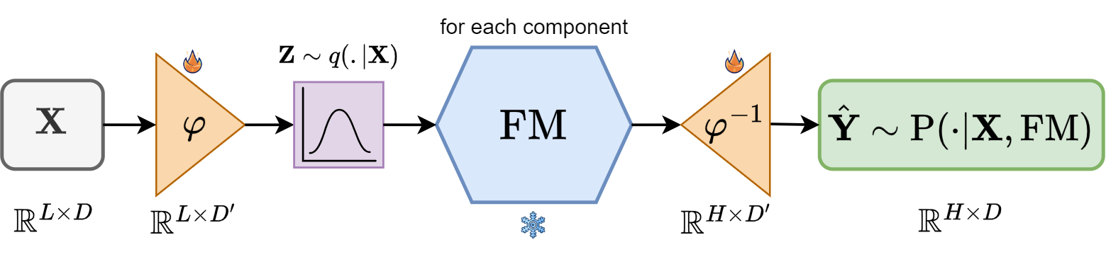
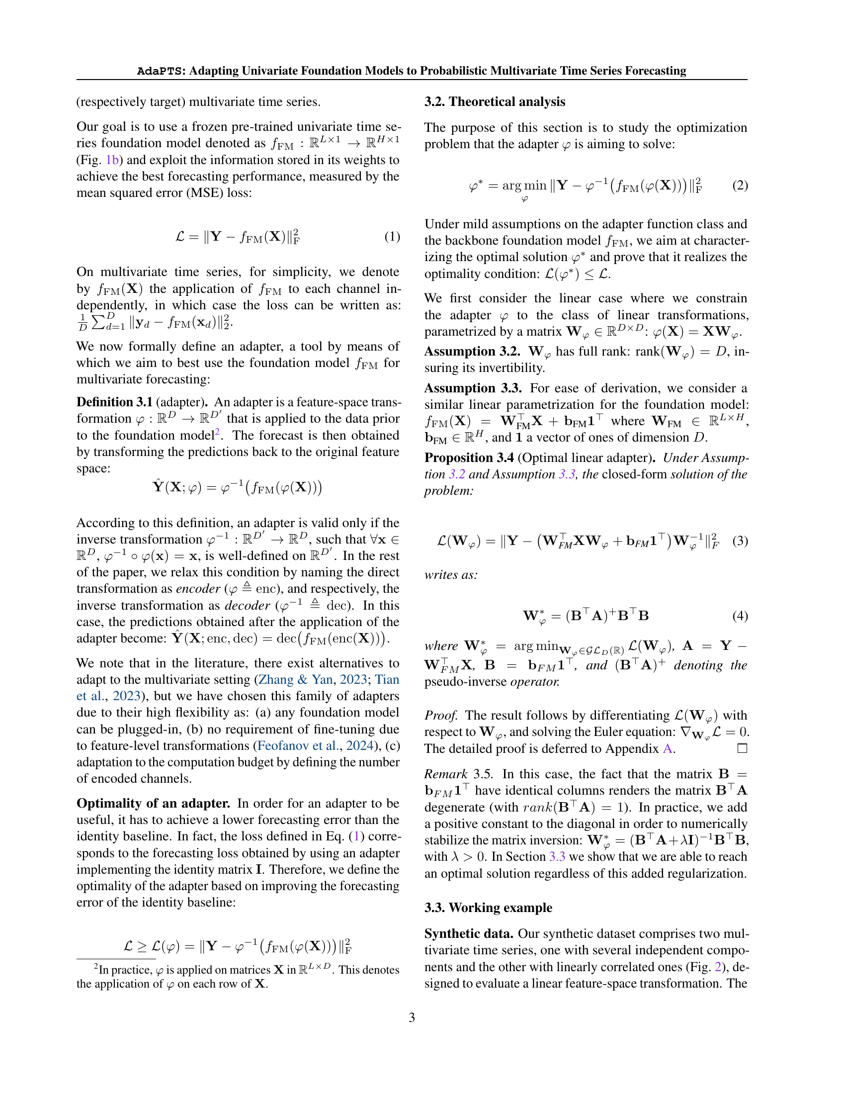
🔼 This figure shows the AdaPTS framework’s architecture. A multivariate time series (X) is input. An adapter (phi) projects it into a stochastic latent space (Z), which is then fed into a pre-trained univariate foundation model (FM). The model’s output in the latent space is then inversely projected by the adapter’s inverse function (phi^-1) to obtain a probabilistic prediction (Y) in the original feature space. The diagram uses a fire symbol to indicate trainable weights and a snowflake to indicate frozen parameters from the FM.
read the caption
(b)

🔼 Figure 1 illustrates the AdaPTS framework and its application. Panel (a) shows an example of how AdaPTS improves predictions by adding probability and accuracy compared to a standard model. Panel (b) details the framework’s architecture. A multivariate input time series is first transformed into a lower-dimensional stochastic latent space using a learnable feature transformation φ. Then, a pre-trained univariate foundation model (FM) processes each dimension independently in this latent space. Finally, an inverse transformation maps the predictions back into the original multivariate space, producing a probabilistic forecast. The figure uses visual cues to distinguish trainable parameters (fire symbol) from frozen parameters of the FM (snowflake).
read the caption
Figure 1: (a) Augmenting Moment time series foundation model with the AdaPTS framework provides probabilistic and more accurate predictions. (b) The AdaPTS framework: The input time series is transformed through a feature space transformation φ𝜑\varphiitalic_φ that maps into a stochastic latent space. The prediction is then conducted using a pre-trained FM before transforming back the predicted, now distribution, to the original feature space. The fire symbol indicate trainable weights while the snowflake implicates that the parameters of the FM are kept frozen.

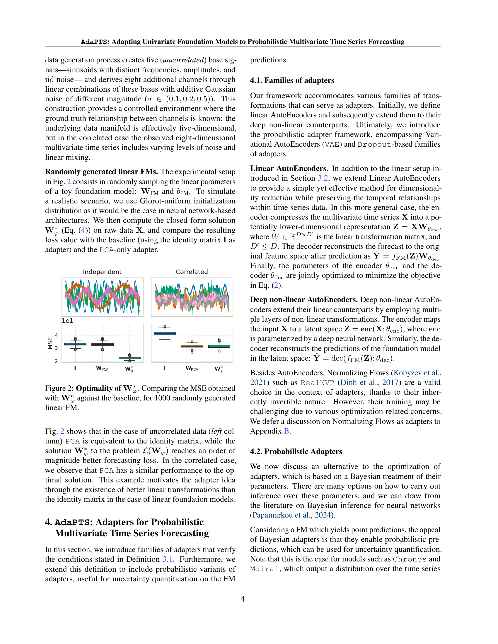
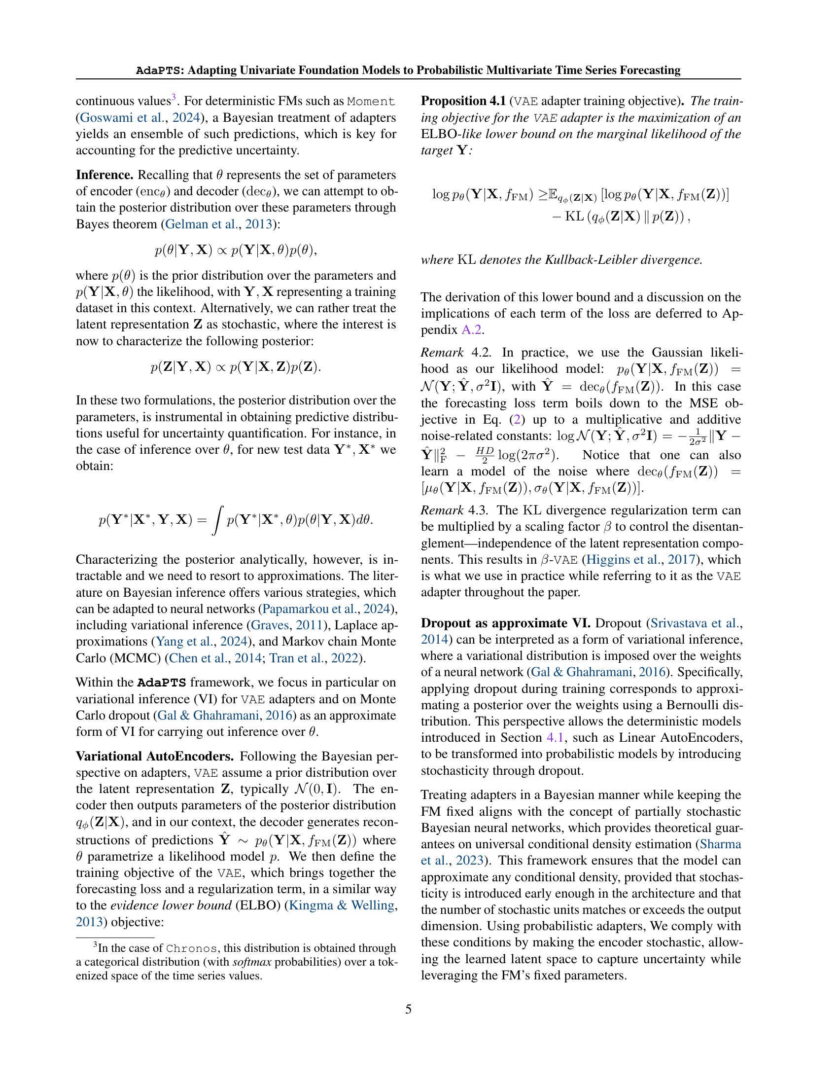
🔼 This figure demonstrates the superiority of the optimal linear adapter, represented as (\mathbf{W}{\varphi}^{*}), over a baseline approach for multivariate time series forecasting. 1000 linear foundation models (FMs) were randomly generated. For each FM, the mean squared error (MSE) was calculated using both the optimal adapter (\mathbf{W}{\varphi}^{}) and a baseline (identity matrix). The results show that (\mathbf{W}_{\varphi}^{}) consistently achieves lower MSE, indicating its effectiveness in improving forecasting accuracy compared to the baseline.
read the caption
Figure 2: Optimality of 𝐖φ∗superscriptsubscript𝐖𝜑\mathbf{W}_{\varphi}^{*}bold_W start_POSTSUBSCRIPT italic_φ end_POSTSUBSCRIPT start_POSTSUPERSCRIPT ∗ end_POSTSUPERSCRIPT. Comparing the MSE obtained with 𝐖φ∗superscriptsubscript𝐖𝜑\mathbf{W}_{\varphi}^{*}bold_W start_POSTSUBSCRIPT italic_φ end_POSTSUBSCRIPT start_POSTSUPERSCRIPT ∗ end_POSTSUPERSCRIPT against the baseline, for 1000 randomly generated linear FM.

🔼 This figure displays the effect of varying the number of components within the adapter on the model’s forecasting accuracy, using the Mean Squared Error (MSE) as a metric. The results are shown for four different datasets (ETTh1, Illness, Weather, and ExchangeRate) across various prediction horizons (H). The dashed line represents the baseline performance of the Moment model without any adapters. The shaded region surrounding this line indicates the standard deviation. The vertical line marks the number of original features in the input dataset. This visualization helps to understand the optimal number of components needed for each adapter to balance model complexity and predictive performance.
read the caption
Figure 3: Impact of the number of components on model performance. The dashed line indicates Moment performance without adapters, the shaded area its standard deviation, and the vertical line the number of original features.

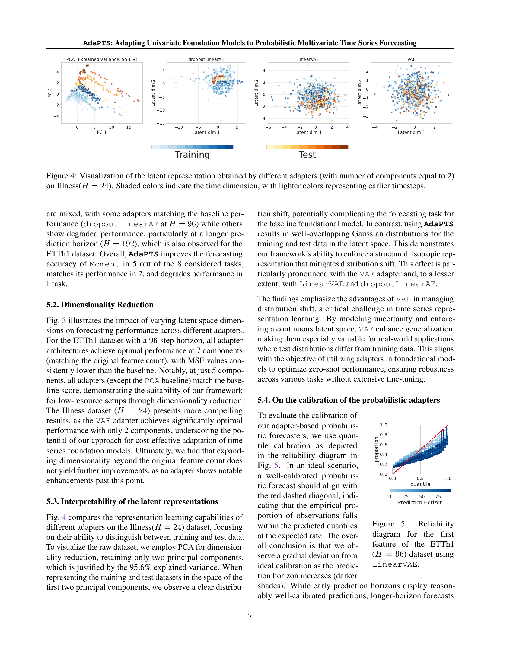
🔼 This figure visualizes the latent representations learned by different adapter types (PCA, dropoutLinearAE, LinearVAE, and VAE) when applied to the Illness dataset with a prediction horizon of 24 time steps. Each adapter reduces the dimensionality of the input data to two components. The plot shows a scatter plot of the latent representations, where the shading of each point indicates the time step within the sequence. Lighter colors correspond to earlier time points in the sequence, and darker colors to later time points. This visualization allows for the comparison of the distinct latent spaces generated by each adapter, highlighting the effects of each adapter on the data’s structure and distribution.
read the caption
Figure 4: Visualization of the latent representation obtained by different adapters (with number of components equal to 2) on Illness(H=24𝐻24H=24italic_H = 24). Shaded colors indicate the time dimension, with lighter colors representing earlier timesteps.

🔼 This reliability diagram visualizes the calibration of probabilistic forecasts generated by the LinearVAE adapter for the first feature of the ETTh1 dataset with a prediction horizon of 96 time steps. It plots the observed proportion of instances where the predicted quantile range contains the actual value against the predicted quantile. A perfectly calibrated model would show a diagonal line, indicating that predictions align with observed values. Deviations from this diagonal reveal over- or underestimation of uncertainty at different quantiles.
read the caption
Figure 5: Reliability diagram for the first feature of the ETTh1 (H=96𝐻96H=96italic_H = 96) dataset using LinearVAE.

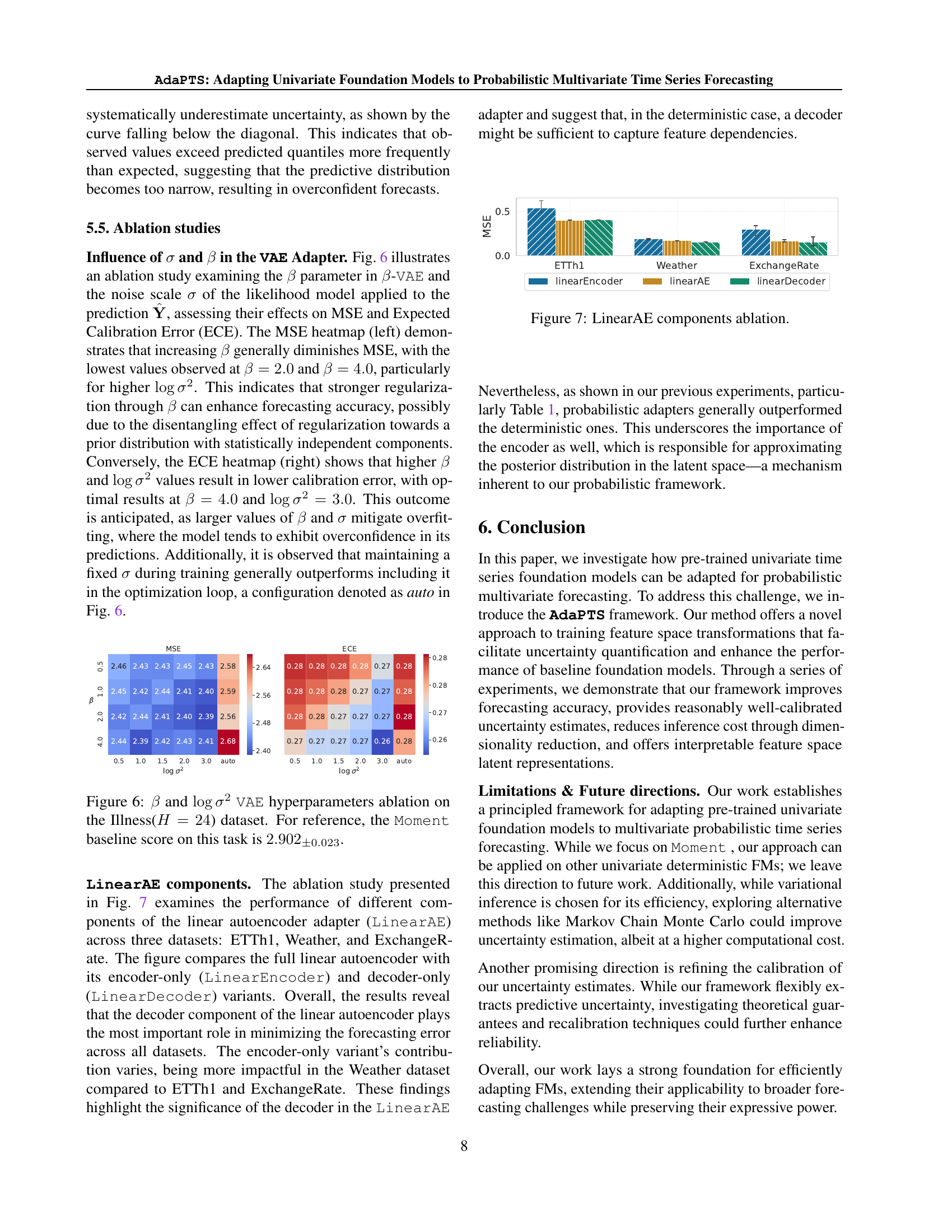
🔼 This figure shows the results of an ablation study on the VAE adapter’s hyperparameters: β (beta), which controls the disentanglement of the latent representation, and log σ² (log sigma squared), representing the noise scale in the likelihood model. The heatmaps illustrate how different combinations of β and log σ² affect the Mean Squared Error (MSE) and Expected Calibration Error (ECE) on the Illness dataset with a forecasting horizon of 24 time steps. Lower MSE values indicate better forecasting accuracy, and lower ECE values suggest better calibration (confidence matches accuracy). The study examines the impact of these hyperparameters on both MSE and ECE, providing insights into how their tuning affects performance and calibration. The baseline MSE score for the Illness dataset is also given as a reference.
read the caption
Figure 6: β𝛽\betaitalic_β and logσ2superscript𝜎2\log\sigma^{2}roman_log italic_σ start_POSTSUPERSCRIPT 2 end_POSTSUPERSCRIPT VAE hyperparameters ablation on the Illness(H=24𝐻24H=24italic_H = 24) dataset. For reference, the Moment baseline score on this task is 2.902±0.023subscript2.902plus-or-minus0.0232.902_{\pm 0.023}2.902 start_POSTSUBSCRIPT ± 0.023 end_POSTSUBSCRIPT.

🔼 This ablation study investigates the individual contributions of the encoder and decoder components within the Linear AutoEncoder (LinearAE) adapter architecture. The experiment compares the full LinearAE against versions using only the encoder (LinearEncoder) or only the decoder (LinearDecoder). The results show the impact of each component on forecasting accuracy across three datasets: ETTh1, Weather, and ExchangeRate. This helps to understand which part of the LinearAE plays the most crucial role in improving the forecasting performance and whether the inclusion of both encoder and decoder is necessary for optimal results.
read the caption
Figure 7: LinearAE components ablation.

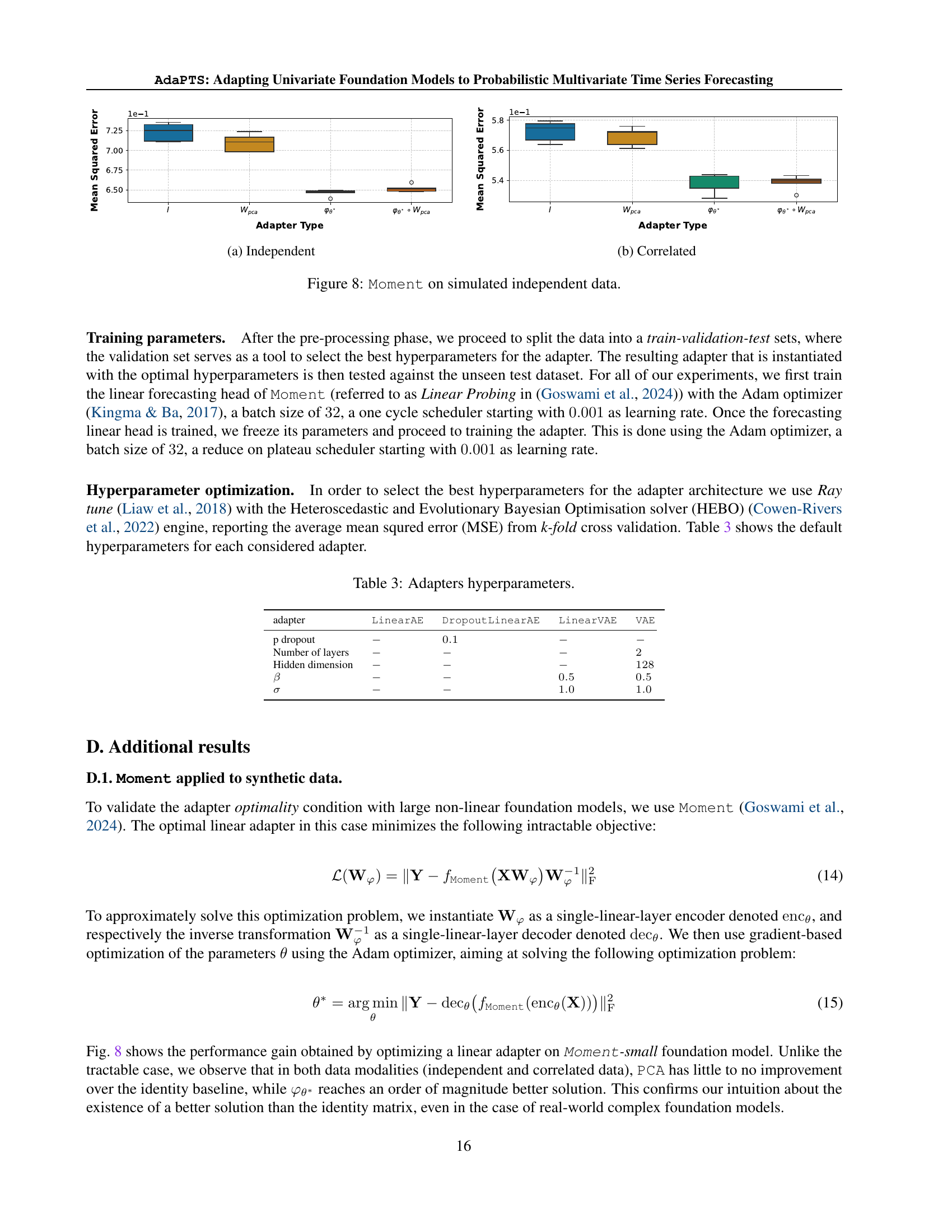
🔼 This figure displays the results of applying the Moment model to synthetic datasets, specifically focusing on the Mean Squared Error (MSE). Subfigure (a) showcases the MSE for a synthetic dataset with independent components. The comparison includes the results of using PCA as an adapter, the adapter with parameters learned directly (θ), and the composition of the learned parameters with PCA (θ* • Wpca). The x-axis represents the type of adapter used, while the y-axis shows the MSE. Subfigure (b) shows the same comparison but uses a correlated synthetic dataset.
read the caption
(a) Independent

🔼 This figure shows the mean squared error (MSE) achieved by different adapter methods on a synthetic dataset with correlated features. The x-axis represents different adapter types, including the baseline (PCA), and the proposed linear adapters. The y-axis represents the MSE values. The figure illustrates that the proposed linear adapter (Wφ) outperforms other methods, including PCA, in terms of MSE, indicating its effectiveness in improving forecasting accuracy in multivariate time series with complex inter-feature relationships.
read the caption
(b) Correlated

🔼 This figure displays the mean squared error (MSE) achieved by different adapter types when applied to the Moment model on simulated independent and correlated datasets. The x-axis represents the adapter type, including the baseline PCA (Principal Component Analysis) and the proposed methods. The y-axis represents the MSE. The plot visualizes a comparison between using only PCA, a standard linear adapter, and a combination of PCA and a learned linear adapter. The results illustrate the efficacy of the proposed adapters, showing that the combination of PCA and the learned adapter significantly reduces MSE compared to the baseline methods, particularly on the correlated dataset.
read the caption
Figure 8: Moment on simulated independent data.
More on tables
| Dataset | ETTh1 | Illness | ExchangeRate | Weather |
| # features | ||||
| # time steps | ||||
| Granularity | 1 hour | 1 week | 1 day | 10 minutes |
| (Train, Val, Test) | (8033, 2785, 2785) | (69, 2, 98) | (4704, 665, 1422) | (36280, 5175, 10444) |
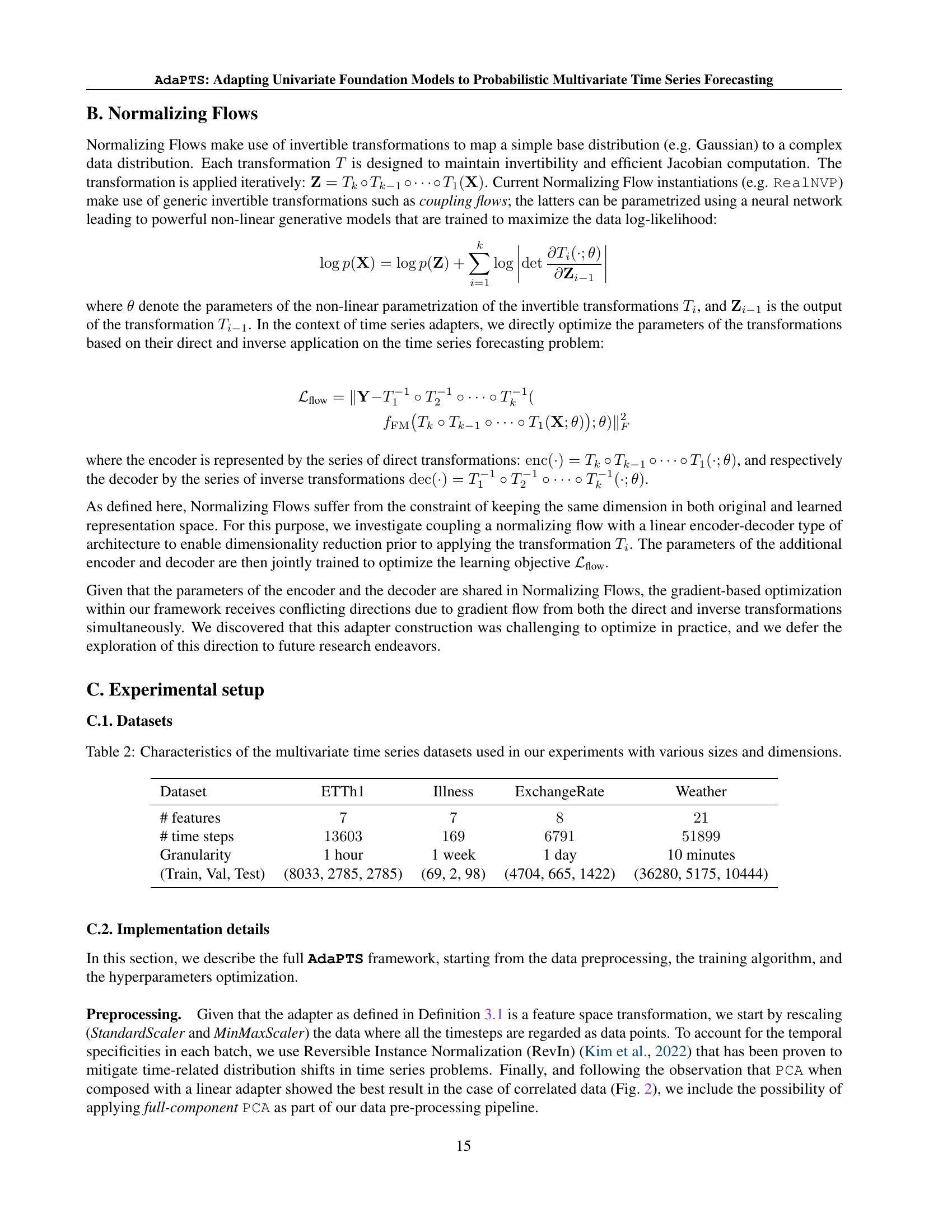
🔼 This table presents the characteristics of four multivariate time series datasets used in the paper’s experiments. For each dataset, it lists the number of features, the total number of time steps, the granularity of the time steps (e.g., hourly, daily), and the size of the training, validation, and test sets. This information is crucial for understanding the scale and nature of the data used in evaluating the proposed methodology.
read the caption
Table 2: Characteristics of the multivariate time series datasets used in our experiments with various sizes and dimensions.
| adapter | LinearAE | DropoutLinearAE | LinearVAE | VAE |
| p dropout | ||||
| Number of layers | ||||
| Hidden dimension | ||||
🔼 This table lists the hyperparameters used for each type of adapter in the AdaPTS framework. It shows the values used for the number of layers, hidden dimension, beta (β) for beta-VAE, and sigma (σ) for the VAE and LinearVAE adapters. These hyperparameters were tuned to optimize the performance of each adapter architecture.
read the caption
Table 3: Adapters hyperparameters.
| Dataset | H | No adapter | with adapter | ||||
| pca | linear | dropout | linear VAE | VAE | |||
| ETTh1 | 96 | ||||||
| 192 | |||||||
| Illness | 24 | ||||||
| 60 | |||||||
| Weather | 96 | ||||||
| 192 | |||||||
| ExchangeRate | 96 | ||||||
| 192 | |||||||
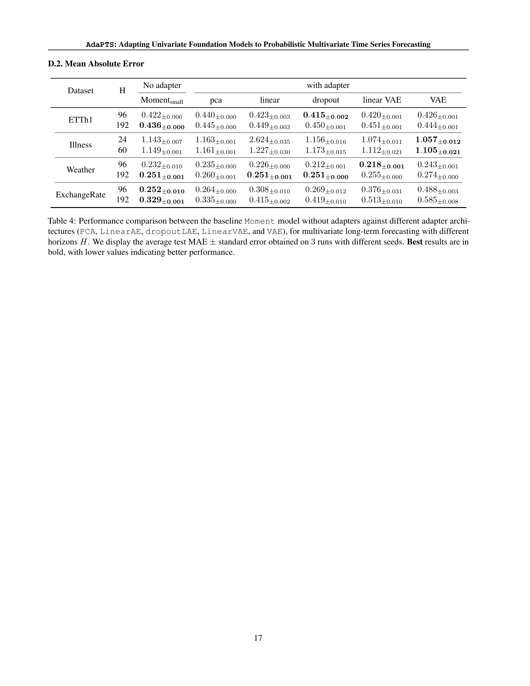
🔼 Table 4 presents a detailed comparison of the forecasting accuracy achieved by different methods on four real-world multivariate time series datasets. The results are broken down by dataset (ETTh1, Illness, Weather, ExchangeRate), prediction horizon (H), and forecasting method. The methods compared include Moment (a baseline model without adapters), PCA (principal component analysis as an adapter), LinearAE (linear autoencoder), dropoutLAE (linear autoencoder with dropout), LinearVAE (linear variational autoencoder), and VAE (variational autoencoder). The primary metric used for evaluation is Mean Absolute Error (MAE). For each dataset and horizon, the table provides the average MAE across three runs, each initialized with different random seeds, along with the associated standard error to show the reliability of the results. The best-performing method for each dataset and horizon is highlighted in bold, emphasizing the relative effectiveness of each adapter type.
read the caption
Table 4: Performance comparison between the baseline Moment model without adapters against different adapter architectures (PCA, LinearAE, dropoutLAE, LinearVAE, and VAE), for multivariate long-term forecasting with different horizons H𝐻Hitalic_H. We display the average test MAE ±plus-or-minus\pm± standard error obtained on 3333 runs with different seeds. Best results are in bold, with lower values indicating better performance.
Full paper#