TL;DR#
Creating realistic animations from 3D models traditionally requires manually adding skeletons and skinning weights, a time-consuming and labor-intensive process. The lack of large-scale datasets has also hindered the development of automated solutions. This paper presents significant challenges in current 3D animation pipelines.
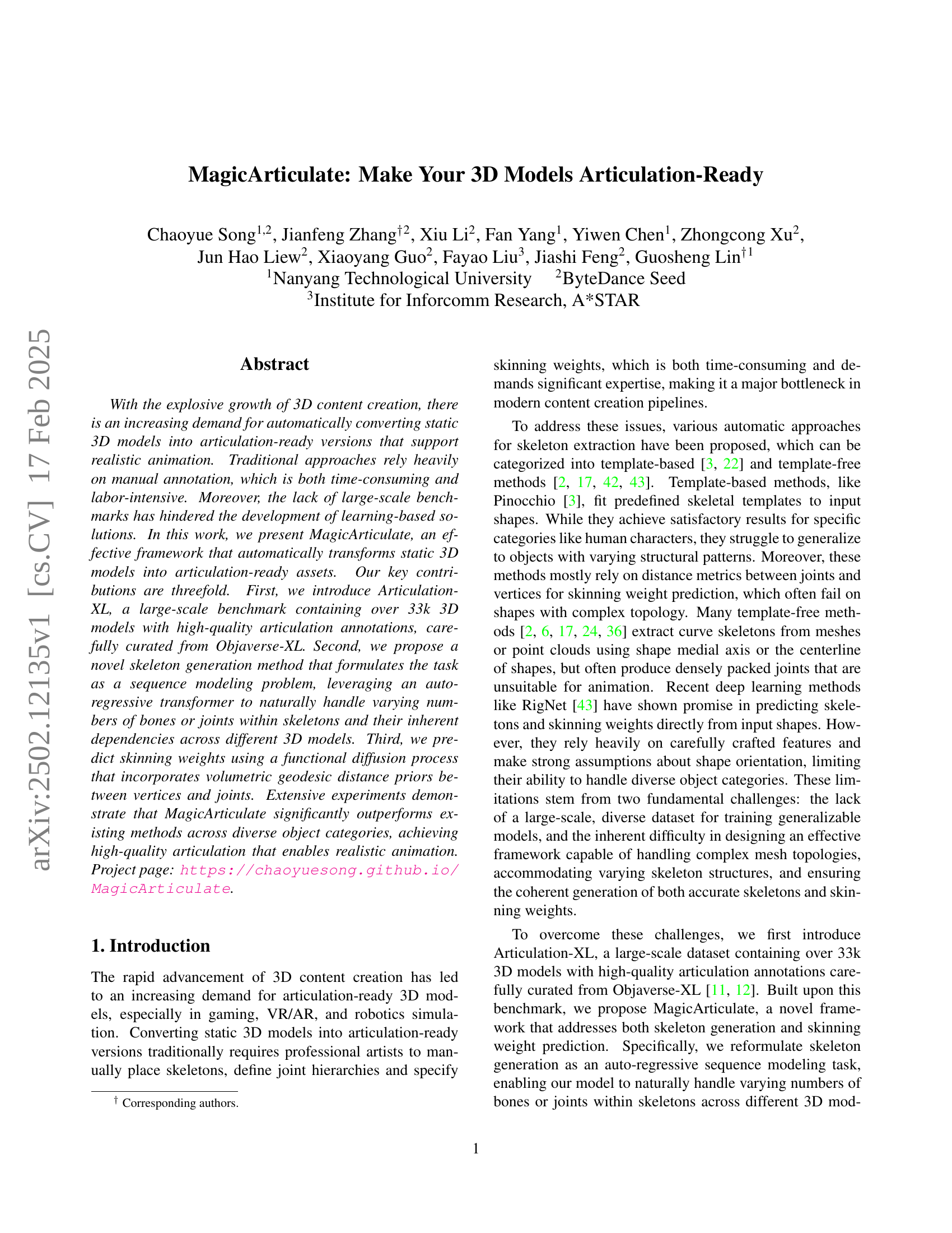
The paper introduces MagicArticulate, a novel framework that addresses these challenges. It uses an auto-regressive transformer for skeleton generation, handling varying bone numbers efficiently. Skinning weights are predicted using a functional diffusion process that incorporates volumetric geodesic distance priors, improving accuracy on complex topologies. MagicArticulate significantly outperforms existing methods across diverse object categories, achieving high-quality articulation for realistic animation. The paper also introduces Articulation-XL, a substantial benchmark dataset to facilitate future research.
Key Takeaways#
Why does it matter?#
This paper is crucial because it addresses a critical bottleneck in 3D content creation: the time-consuming manual process of making 3D models animation-ready. By introducing a novel automated framework and a large-scale benchmark dataset, it significantly accelerates the workflow and opens exciting avenues for research in computer graphics and animation. This will benefit researchers across diverse fields utilizing 3D models, including gaming, VR/AR, and robotics.
Visual Insights#

🔼 This figure showcases the capabilities of MagicArticulate. Given three different 3D models (a boy, a giraffe, and a dog), the system automatically generates a corresponding skeleton and computes skinning weights, which are necessary for realistic animation. The input 3D models themselves were created using Rodin Gen-1 and Tripo 2.0, and the resulting images were produced using the Maya Software Renderer. This demonstrates the system’s ability to prepare 3D models for animation without manual intervention.
read the caption
Figure 1: Given a 3D model, MagicArticulate can automatically generate the skeleton and skinning weights, making the model articulation-ready without further manual refinement. The input meshes are generated by Rodin Gen-1 [50] and Tripo 2.0 [1]. The meshes and skeletons are rendered using Maya Software Renderer [19].
| Dataset | CD-J2J | CD-J2B | CD-B2B | |
| RigNet* | ModelsRes. | 7.132 | 5.486 | 4.640 |
| Pinocchio | 6.852 | 4.824 | 4.089 | |
| Ours-hier* | 4.451 | 3.454 | 2.998 | |
| RigNet | 4.143 | 2.961 | 2.675 | |
| Ours-spatial* | 4.103 | 3.101 | 2.672 | |
| Ours-hier | 3.654 | 2.775 | 2.412 | |
| Ours-spatial | 3.343 | 2.455 | 2.140 | |
| Pinocchio | Arti-XL | 8.360 | 6.677 | 5.689 |
| RigNet | 7.478 | 5.892 | 4.932 | |
| Ours-hier | 3.025 | 2.408 | 2.083 | |
| Ours-spatial | 2.586 | 1.959 | 1.661 |
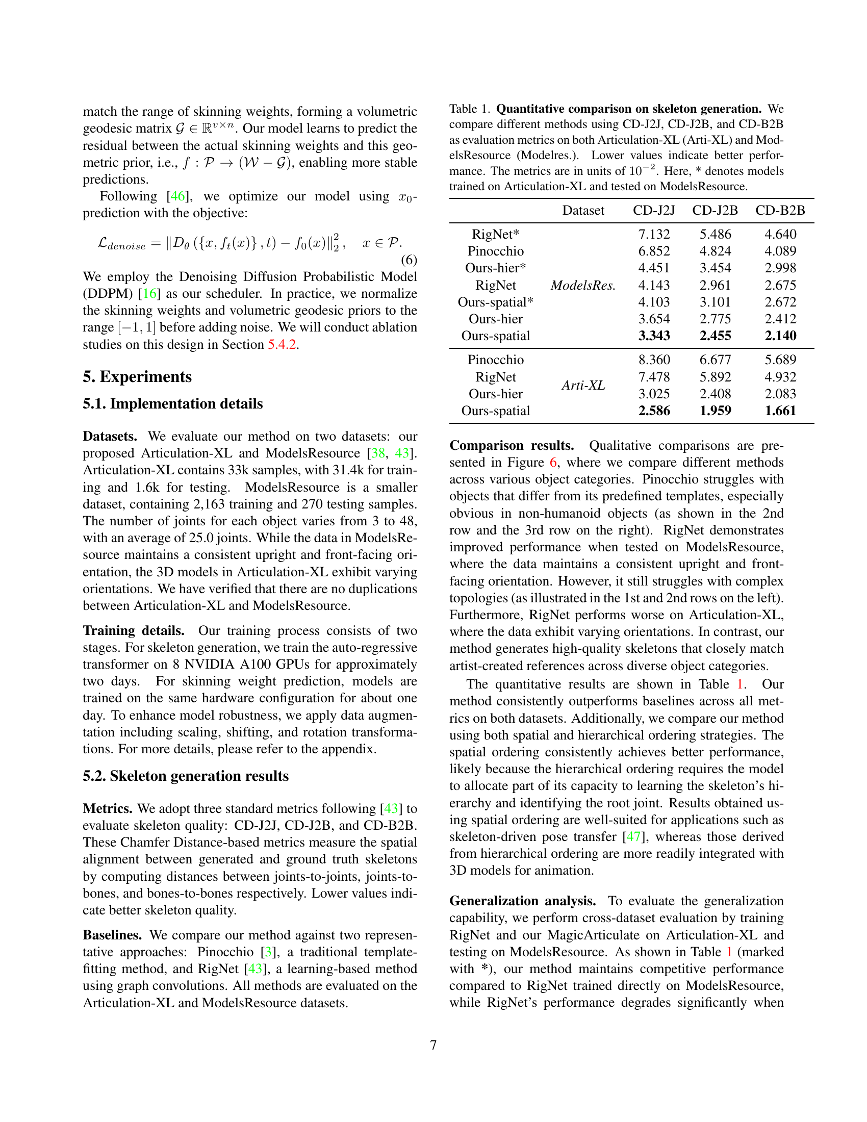
🔼 This table presents a quantitative comparison of different methods for skeleton generation. The comparison uses three Chamfer distance metrics (CD-J2J, CD-J2B, and CD-B2B) to evaluate the accuracy of generated skeletons against ground truth skeletons. Results are shown for two datasets: Articulation-XL and ModelsResource. Lower values for each metric indicate better performance. The table also notes that some models were trained on Articulation-XL and then tested on ModelsResource, indicated by an asterisk (*).
read the caption
Table 1: Quantitative comparison on skeleton generation. We compare different methods using CD-J2J, CD-J2B, and CD-B2B as evaluation metrics on both Articulation-XL (Arti-XL) and ModelsResource (Modelres.). Lower values indicate better performance. The metrics are in units of 10−2superscript10210^{-2}10 start_POSTSUPERSCRIPT - 2 end_POSTSUPERSCRIPT. Here, * denotes models trained on Articulation-XL and tested on ModelsResource.
In-depth insights#
Articulation-XL Dataset#
The Articulation-XL dataset represents a significant contribution to the field of 3D model articulation. Its large scale, exceeding 33,000 3D models, addresses a critical limitation in previous research, namely the scarcity of sufficiently large and diverse datasets for training robust learning-based methods. The high-quality articulation annotations included, carefully curated from Objaverse-XL, are crucial for model evaluation and ensure reliable training data. The dataset’s diversity, encompassing various object categories with different bone counts and joint structures, enables the development of truly generalizable models that can handle the complexity and variations inherent in real-world 3D objects. Further, its comprehensive metadata and readily available format should ease reproducibility and accelerate future research in articulated object generation and animation. The inclusion of category labels, obtained through VLM annotation, adds further value, facilitating analysis and enabling researchers to explore specific object types and articulation patterns. Articulation-XL’s impact is far-reaching, providing a robust benchmark for evaluating progress in automatic skeleton generation, skinning weight prediction, and ultimately, realistic 3D animation.
Autoregressive Skeletons#
The concept of “Autoregressive Skeletons” in 3D model articulation presents a novel approach to skeletal generation. Instead of relying on predefined templates or heuristic methods, an autoregressive model learns to predict the skeletal structure sequentially, bone by bone. This allows for handling the variability in the number and arrangement of bones across different object categories. The autoregressive nature naturally captures the dependencies between bones, creating more realistic and coherent skeletons. This approach is particularly advantageous when dealing with complex, diverse shapes where traditional methods struggle. Furthermore, using an autoregressive approach enables the model to adapt dynamically to each object’s unique structure, providing flexibility and scalability. By learning the bone connectivity and spatial relationships in a sequential manner, the model implicitly learns an understanding of skeletal topology and articulation, leading to improved accuracy and generalization capability. A key aspect is the integration of shape information, potentially through a shape encoder, to condition the autoregressive generation, thus ensuring the skeleton aligns well with the 3D model’s geometry. Overall, Autoregressive Skeletons offers a powerful and flexible method for 3D skeletal modeling, overcoming limitations of previous template-based and heuristic approaches.
Diffusion Skinning#
Diffusion models, known for their prowess in image generation, offer a novel approach to skinning weight prediction in 3D models. Instead of directly regressing weights, a diffusion process adds noise to the weight function, gradually transforming it into pure noise. A neural network is then trained to reverse this process, denoising the weights step-by-step to recover the original, smoothly varying skinning weights. This approach offers several advantages. Firstly, it naturally handles complex mesh topologies, unlike traditional methods which often struggle with intricate geometries. Secondly, it elegantly addresses varying skeleton structures, adapting to different numbers of bones and joints. Finally, the functional diffusion framework allows for smooth and coherent weight generation, improving the realism and quality of animation. The incorporation of volumetric geodesic distance priors further enhances the method’s accuracy, guiding the weight prediction towards biologically plausible results. While this approach is promising, further exploration is needed to fully understand the computational cost and the method’s scalability for extremely high-resolution models. Nevertheless, diffusion skinning presents a powerful, data-driven alternative to traditional methods, offering significant potential for advancing the field of 3D character animation.
Method Limitations#
The research paper’s methodology, while innovative, presents several limitations. Data limitations are significant; the Articulation-XL dataset, though large, may not fully represent the vast diversity of 3D model types and articulation styles encountered in real-world applications. Generalization to unseen data is another concern. While the model performs well on the training data, its ability to accurately generate skeletons and skinning weights for completely novel, unseen object types remains uncertain. Computational cost is also a factor; the autoregressive approach, while effective, is computationally expensive, potentially hindering its scalability to larger and more complex datasets. Finally, mesh quality significantly impacts the method’s performance; the model struggles with low-resolution or noisy meshes, highlighting the need for improved robustness to imperfect input data. These limitations suggest future research should focus on addressing these challenges through expanding the dataset’s scope, developing more efficient algorithms, and enhancing robustness to noisy input.
Future Directions#
The research paper’s ‘Future Directions’ section could explore several promising avenues. Improving robustness to diverse object categories is crucial; the current method struggles with complex topologies and unusual shapes. Addressing this requires exploring more sophisticated shape representations and potentially incorporating physics-based modeling into the skeleton generation process. Expanding the dataset to include a wider variety of objects and articulation types is also vital, particularly encompassing those with subtle or highly specific joint structures and behaviors, such as soft robotics or flexible materials. Exploring alternative sequence modeling techniques such as hierarchical or graph-based methods could enhance the model’s capability in capturing complex skeletal structures and interdependencies between joints. Finally, combining the model with other AI techniques, such as text-to-3D generation and physics simulations, would open up new possibilities for creative and realistic animation, streamlining the entire 3D content creation pipeline. Addressing the coarse mesh issue is also paramount; research into more robust mesh processing and input methods is needed. The ultimate goal is a fully automated and highly generalizable system for creating high-fidelity articulation-ready 3D models.
More visual insights#
More on figures

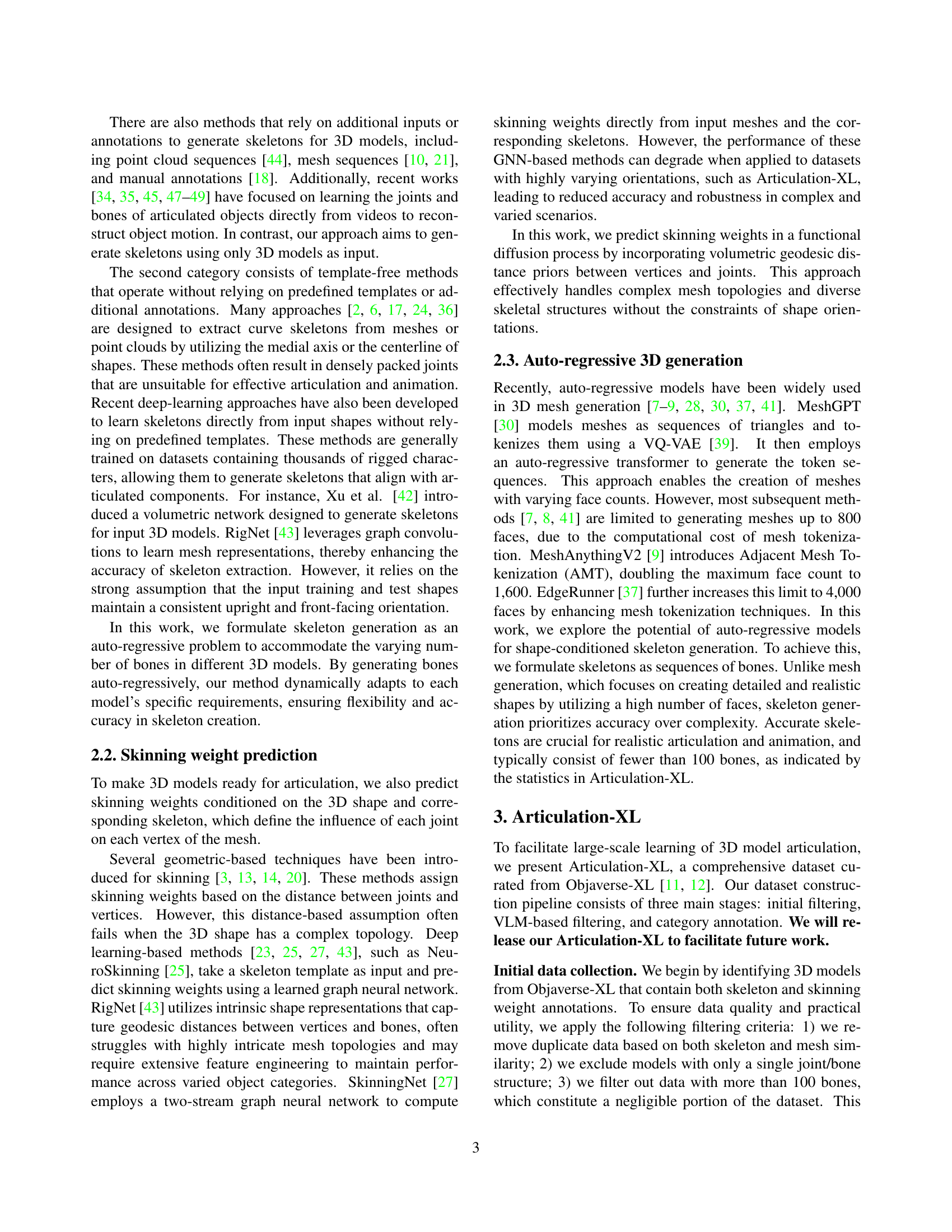
🔼 This figure visualizes the categories of 3D models included in the Articulation-XL dataset using a word cloud. The size of each word is proportional to the frequency of its corresponding category in the dataset. This provides a quick overview of the types of 3D models represented, highlighting the prevalence of certain categories over others.
read the caption
(a) Word cloud of Articulation-XL categories.

🔼 This pie chart shows the distribution of 3D models across different categories in the Articulation-XL dataset. The categories represent the types of objects included in the dataset, such as animals, characters, vehicles, and more. The size of each slice corresponds to the relative proportion of models belonging to that category within the dataset.
read the caption
(b) Breakdown of Articulation-XL categories.

🔼 The figure shows the distribution of the number of bones present in the 3D models within the Articulation-XL dataset. The x-axis represents the number of bones, and the y-axis represents the frequency or count of models with that specific number of bones. This histogram visually illustrates the range and concentration of bone counts across the dataset, providing insights into the complexity and diversity of the 3D model skeletons.
read the caption
(c) Bone number distributions of Articulation-XL.

🔼 This figure presents a statistical overview of the Articulation-XL dataset. It includes a word cloud summarizing the categories of 3D models in the dataset, a pie chart showing the distribution of these categories, and a histogram illustrating the distribution of bone numbers per model. This provides insights into the diversity and complexity of the data.
read the caption
Figure 2: Articulation-XL statistics.

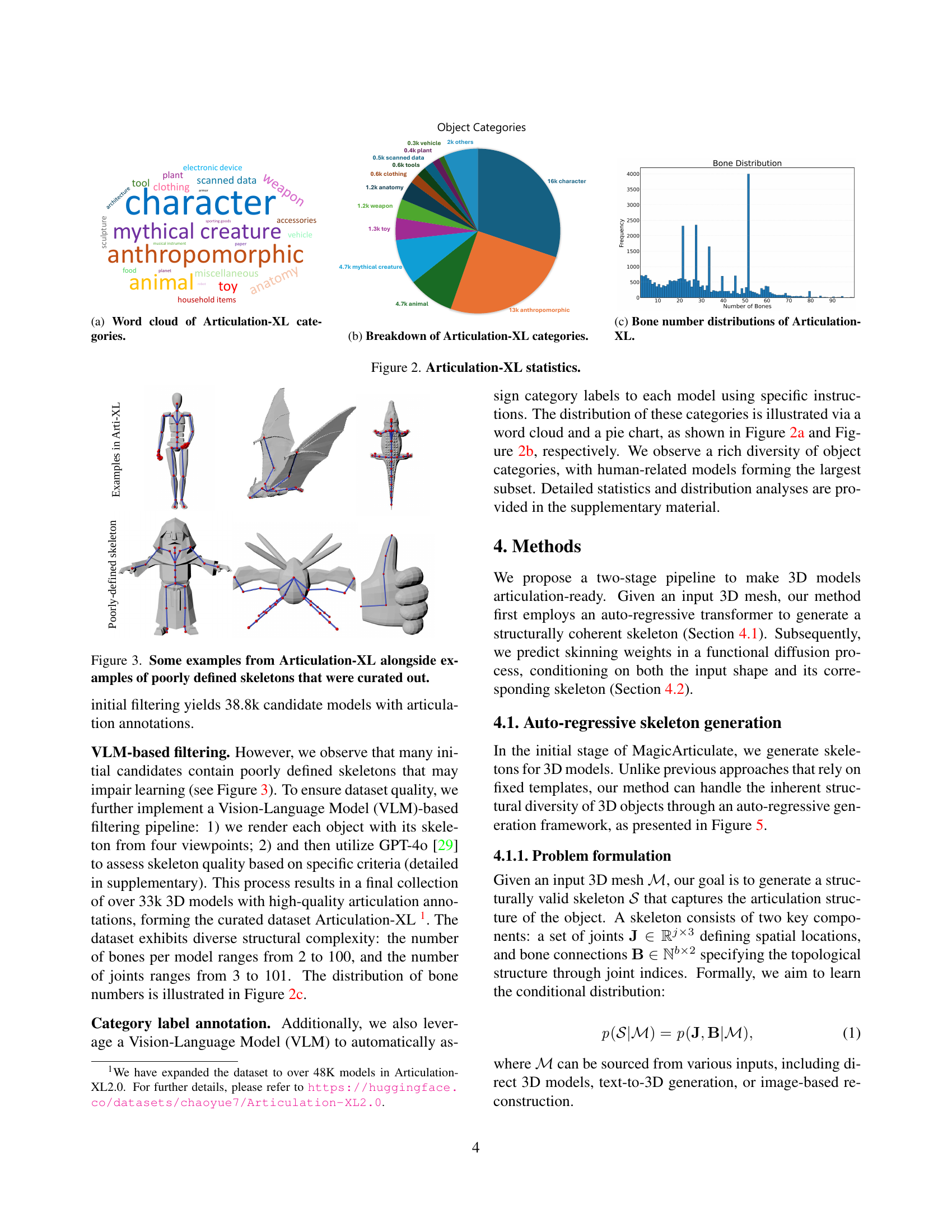
🔼 This figure showcases examples of high-quality 3D models with their corresponding skeletons from the Articulation-XL dataset. It also displays examples of 3D models that were excluded from the dataset due to poorly defined or inaccurate skeletal annotations. This visual comparison highlights the standards for quality control applied in creating the Articulation-XL benchmark.
read the caption
Figure 3: Some examples from Articulation-XL alongside examples of poorly defined skeletons that were curated out.

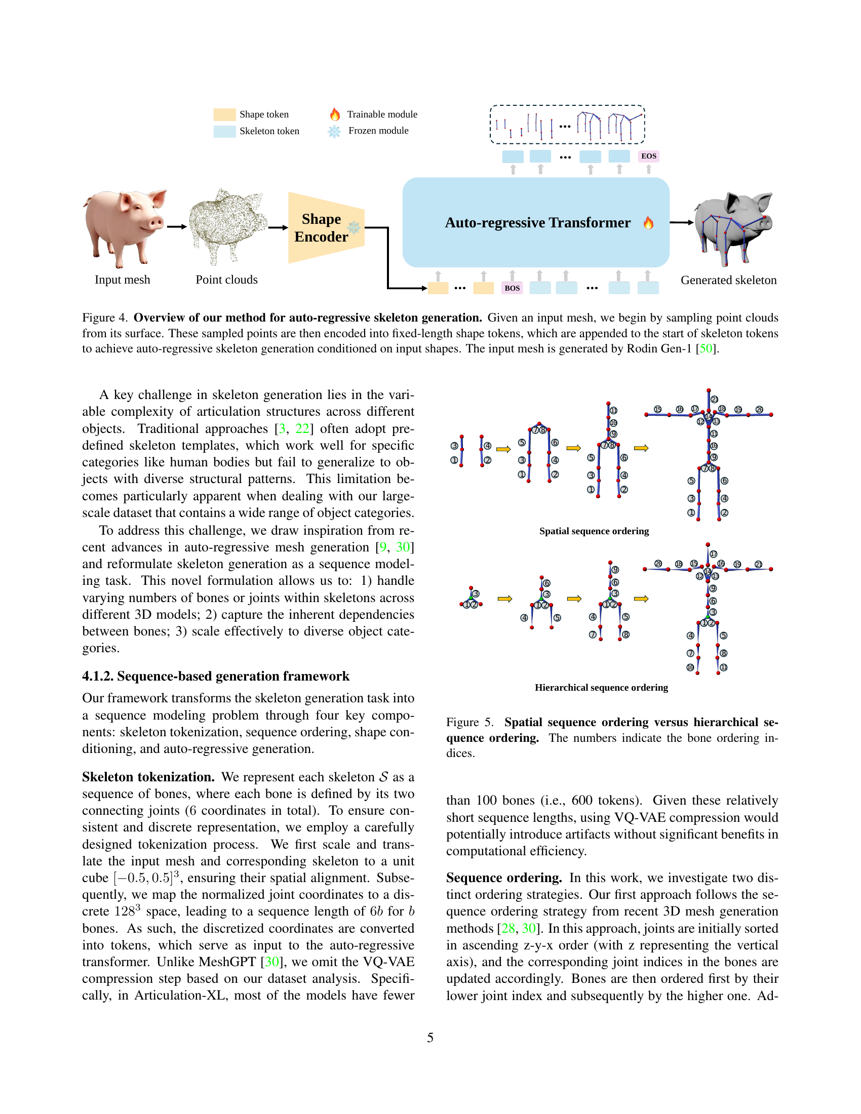
🔼 This figure illustrates the process of autoregressive skeleton generation, a key component of the MagicArticulate framework. The process begins with an input 3D mesh, from which point cloud samples are extracted from the mesh surface. These points are then fed into a shape encoder that generates fixed-length shape tokens. These tokens are concatenated with skeleton tokens, forming the input to an autoregressive transformer. The transformer predicts the skeleton, conditioned on the input shape, generating a sequence of bones and joints that represent the object’s skeletal structure. The output is then a complete articulated skeleton. The input mesh shown in the figure is generated using Rodin Gen-1 [50].
read the caption
Figure 4: Overview of our method for auto-regressive skeleton generation. Given an input mesh, we begin by sampling point clouds from its surface. These sampled points are then encoded into fixed-length shape tokens, which are appended to the start of skeleton tokens to achieve auto-regressive skeleton generation conditioned on input shapes. The input mesh is generated by Rodin Gen-1 [50].

🔼 This figure illustrates two different approaches for ordering bones during skeleton generation: spatial sequence ordering and hierarchical sequence ordering. In spatial ordering, bones are ordered based on the spatial coordinates of their joints, prioritizing z, then y, and finally x coordinates. This approach results in a sequence that doesn’t necessarily reflect the hierarchical relationships within the skeleton. In contrast, hierarchical ordering leverages the bone hierarchy, starting with the root bone and recursively processing child bones layer by layer. This ensures that the ordering respects the parent-child relationships within the skeletal structure. The numbers in the figure represent the bone ordering indices for each method, highlighting the difference in sequencing.
read the caption
Figure 5: Spatial sequence ordering versus hierarchical sequence ordering. The numbers indicate the bone ordering indices.

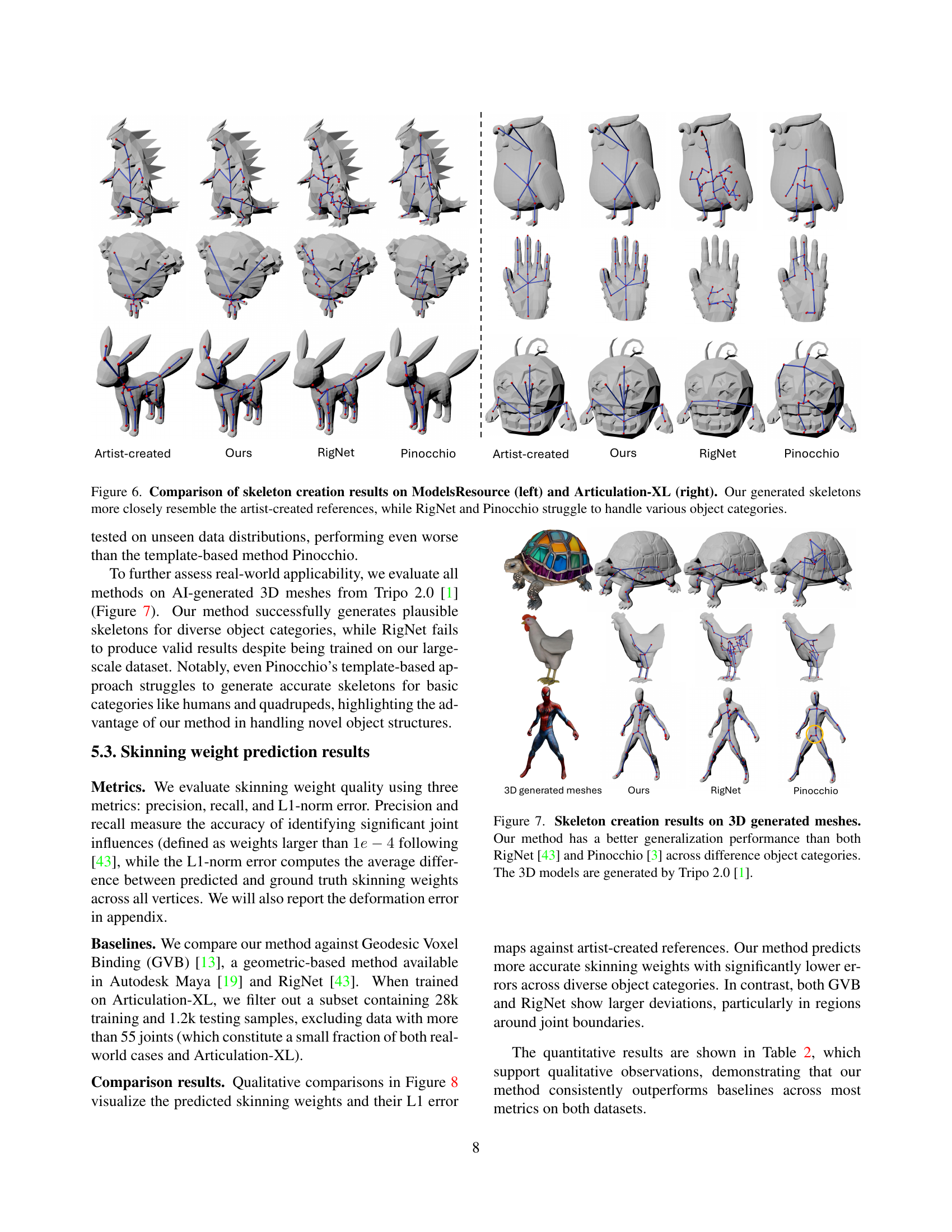
🔼 Figure 6 presents a comparative analysis of skeleton generation results obtained using three different methods: the proposed method (Ours), RigNet, and Pinocchio. The comparison is shown for two datasets: ModelsResource (left column) and Articulation-XL (right column). For each dataset and method, several examples are displayed, showing the automatically generated skeletons alongside the corresponding artist-created reference skeletons. The figure highlights that the proposed method produces skeletons that more accurately reflect the artist-created references, demonstrating improved performance in handling the diverse object categories within the datasets. In contrast, RigNet and Pinocchio exhibit difficulties in generating accurate skeletons, especially for object categories that deviate significantly from the datasets they were trained on.
read the caption
Figure 6: Comparison of skeleton creation results on ModelsResource (left) and Articulation-XL (right). Our generated skeletons more closely resemble the artist-created references, while RigNet and Pinocchio struggle to handle various object categories.

🔼 Figure 7 showcases a comparison of skeleton generation results across various object categories using three different methods: the proposed method, RigNet [43], and Pinocchio [3]. The input 3D models were generated using Tripo 2.0 [1]. The figure demonstrates that the proposed method exhibits superior generalization capabilities compared to RigNet and Pinocchio, producing more accurate and realistic skeletons for a wider variety of object types.
read the caption
Figure 7: Skeleton creation results on 3D generated meshes. Our method has a better generalization performance than both RigNet [43] and Pinocchio [3] across difference object categories. The 3D models are generated by Tripo 2.0 [1].
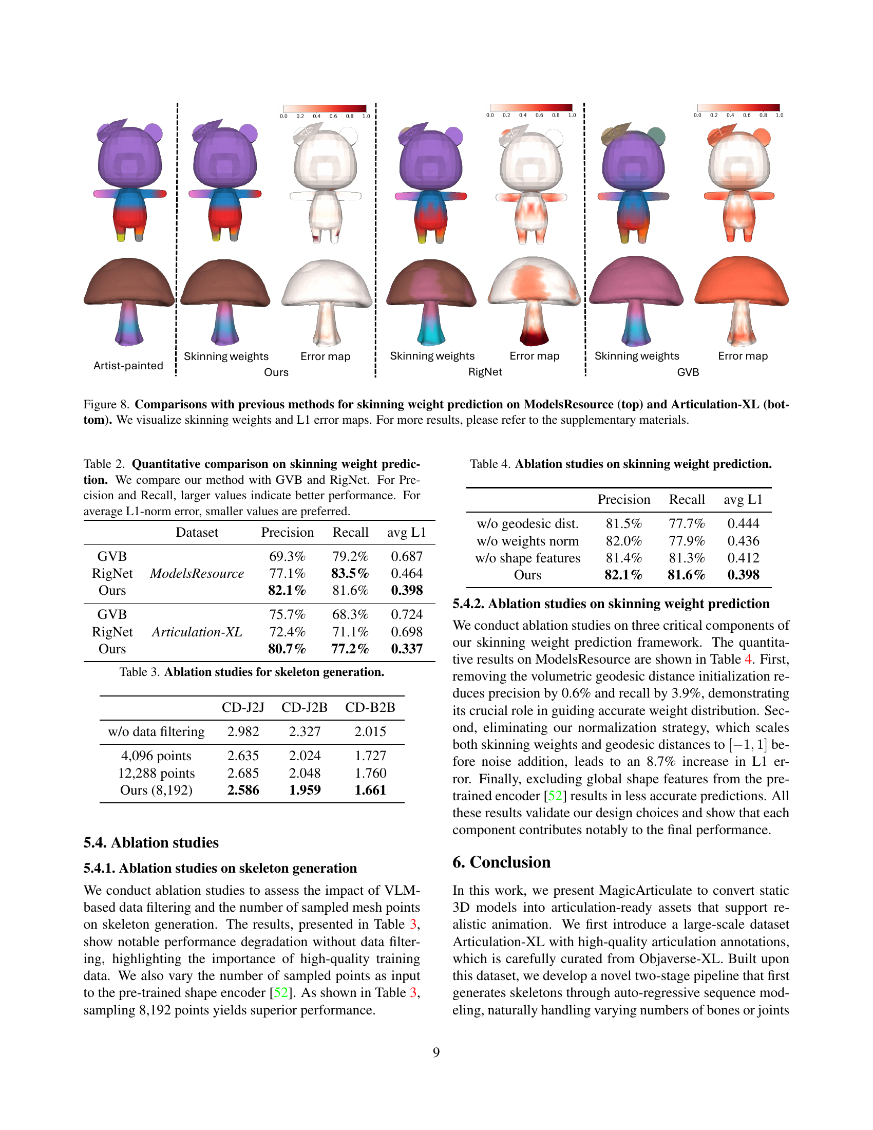
🔼 This figure shows a comparison of skinning weight prediction results between the proposed method and two baseline methods (GVB and RigNet) on two datasets: ModelsResource and Articulation-XL. For each dataset, several example 3D models are displayed. Each model shows the artist-created ground truth skinning weights, along with the skinning weights generated by each method. The accompanying L1 error maps visually represent the difference between the predicted and ground truth skinning weights, with lower values indicating higher accuracy. The figure highlights the superior performance of the proposed method in generating more accurate and realistic skinning weights.
read the caption
Figure 8: Comparisons with previous methods for skinning weight prediction on ModelsResource (top) and Articulation-XL (bottom). We visualize skinning weights and L1 error maps. For more results, please refer to the supplementary materials.

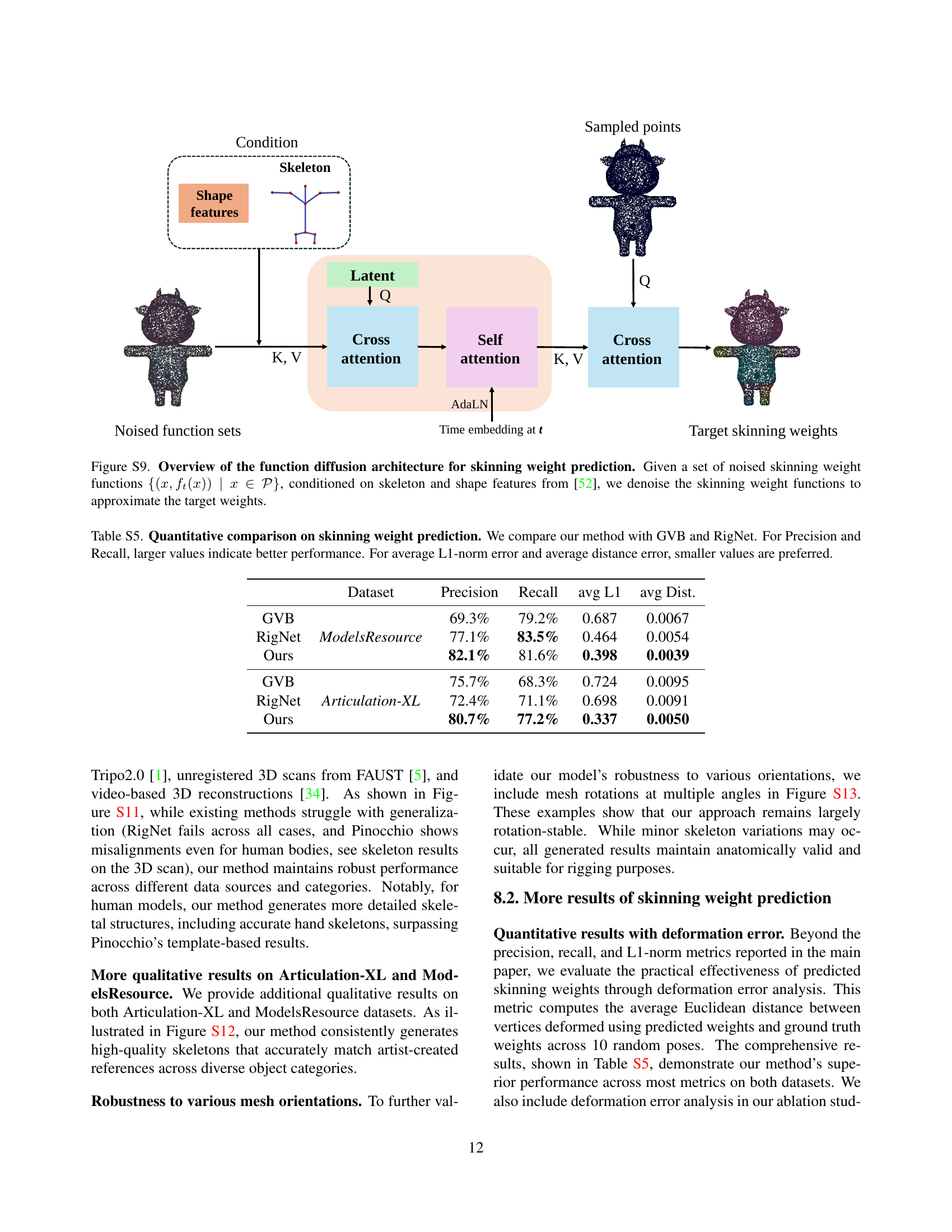
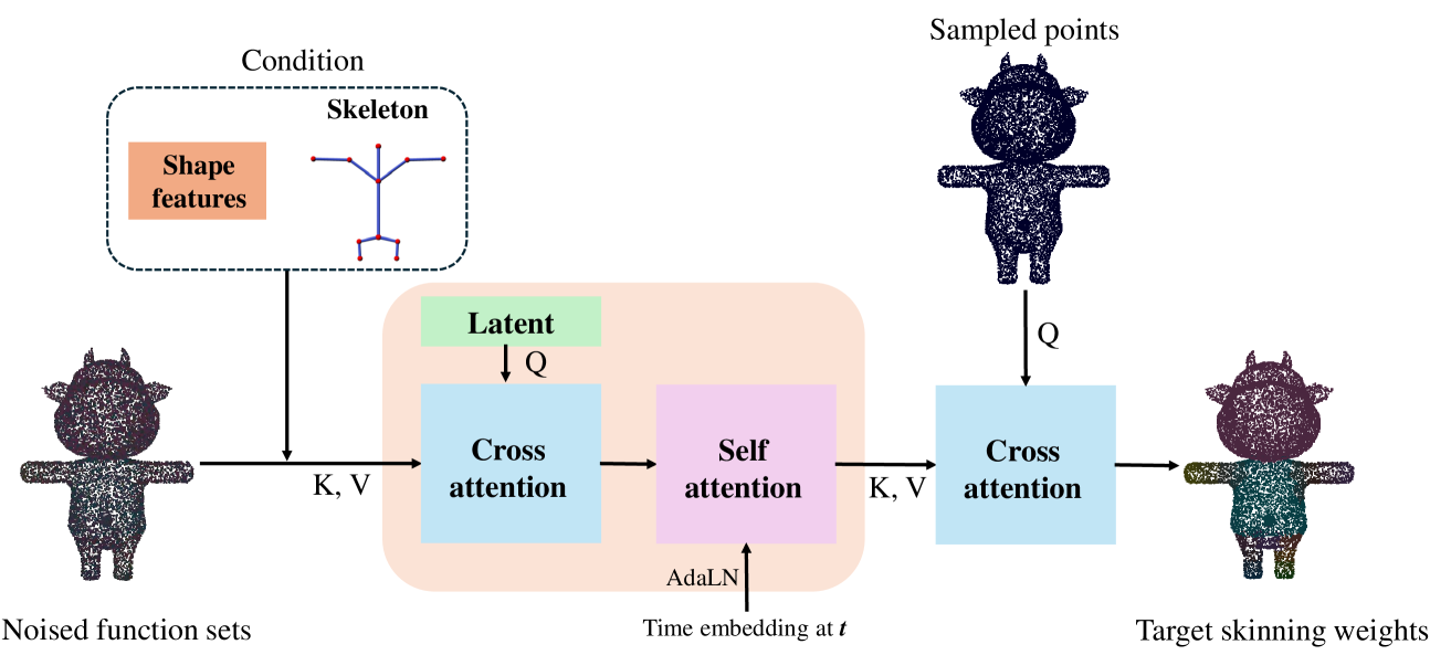
🔼 Figure S9 illustrates the architecture of the functional diffusion model used for skinning weight prediction in MagicArticulate. The model takes as input a set of noisy skinning weight functions, represented as {(x, ft(x)) | x ∈ 𝒫}, where x represents a vertex on the 3D mesh and ft(x) is the noisy skinning weight at that vertex at time step t. Crucially, the model also incorporates both the skeleton and shape features (from a pre-trained encoder, reference [52] in the paper) as conditioning information, which guides the denoising process. The model utilizes cross-attention and self-attention mechanisms to process this combined input and generate a refined set of skinning weights that approximate the target weights.
read the caption
Figure S9: Overview of the function diffusion architecture for skinning weight prediction. Given a set of noised skinning weight functions {(x,ft(x))∣x∈𝒫}conditional-set𝑥subscript𝑓𝑡𝑥𝑥𝒫\{(x,f_{t}(x))\mid x\in\mathcal{P}\}{ ( italic_x , italic_f start_POSTSUBSCRIPT italic_t end_POSTSUBSCRIPT ( italic_x ) ) ∣ italic_x ∈ caligraphic_P }, conditioned on skeleton and shape features from [52], we denoise the skinning weight functions to approximate the target weights.

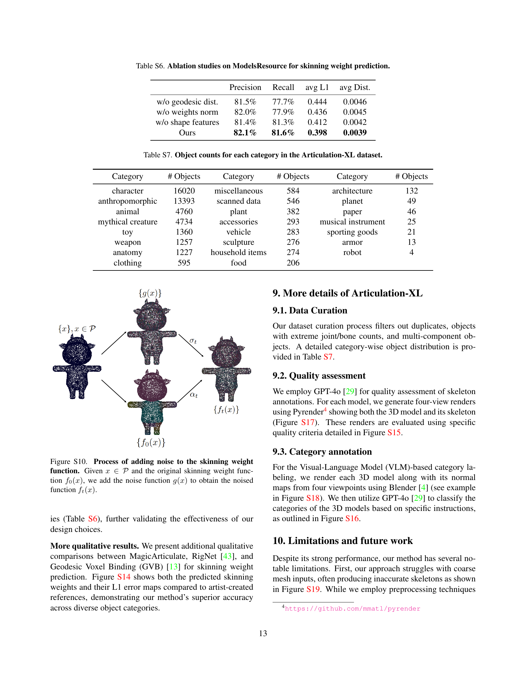
🔼 This figure illustrates the process of adding noise to the skinning weight function during the functional diffusion process for skinning weight prediction. It shows how the original skinning weight function, f₀(x), is modified by adding noise, g(x), to produce the noised function, fₜ(x). The noise level is controlled by the parameter t, which ranges from 0 to 1. This process is a key step in the functional diffusion framework used to predict skinning weights efficiently and accurately for 3D models with complex topologies.
read the caption
Figure S10: Process of adding noise to the skinning weight function. Given x∈𝒫𝑥𝒫x\in\mathcal{P}italic_x ∈ caligraphic_P and the original skinning weight function f0(x)subscript𝑓0𝑥f_{0}(x)italic_f start_POSTSUBSCRIPT 0 end_POSTSUBSCRIPT ( italic_x ), we add the noise function g(x)𝑔𝑥g(x)italic_g ( italic_x ) to obtain the noised function ft(x)subscript𝑓𝑡𝑥f_{t}(x)italic_f start_POSTSUBSCRIPT italic_t end_POSTSUBSCRIPT ( italic_x ).

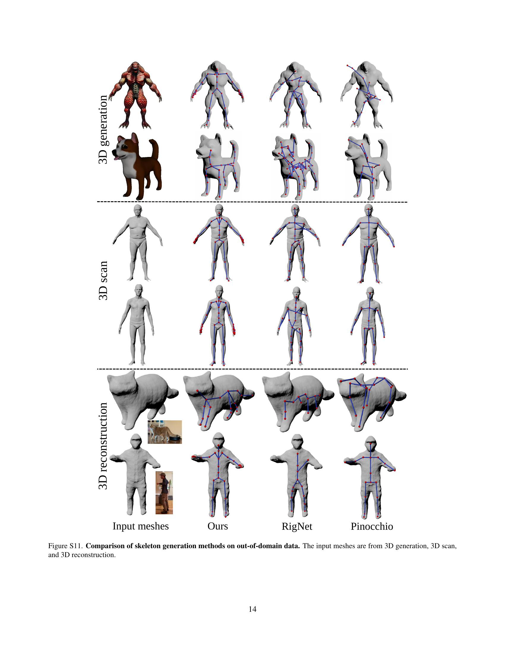
🔼 This figure compares the performance of different skeleton generation methods on 3D models from various sources. The input meshes are obtained from three distinct methods: 3D model generation, 3D scanning, and 3D reconstruction. The comparison showcases how well each method generalizes to different data types and the resulting diversity in 3D model quality, highlighting the strengths and weaknesses of each approach in terms of generating accurate and usable skeletons.
read the caption
Figure S11: Comparison of skeleton generation methods on out-of-domain data. The input meshes are from 3D generation, 3D scan, and 3D reconstruction.

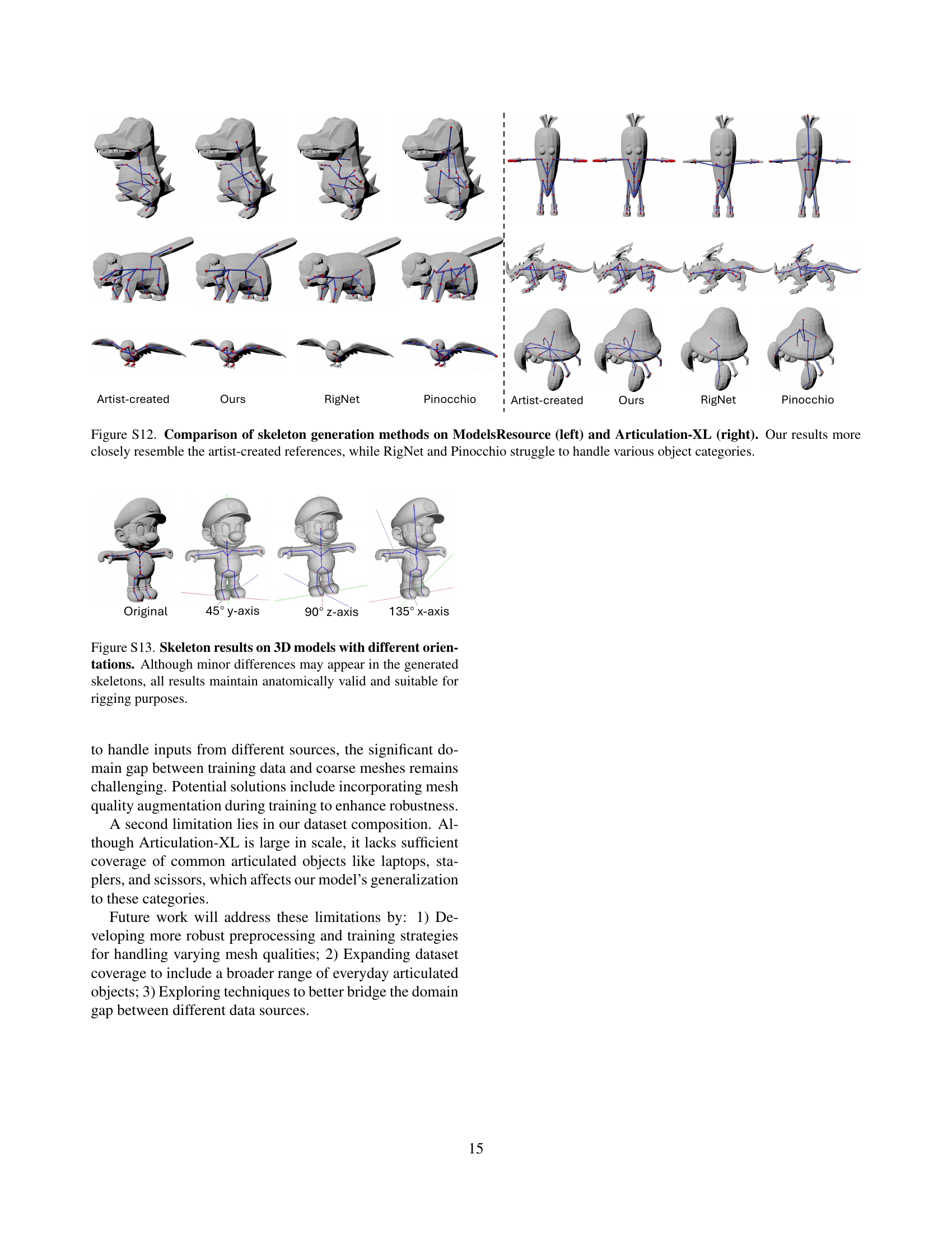
🔼 This figure showcases a qualitative comparison of skeleton generation methods. The left side presents results on the ModelsResource dataset, while the right shows results from the larger, more diverse Articulation-XL dataset. For each dataset, results are displayed for three methods: artist-created skeletons (ground truth), results from the authors’ proposed MagicArticulate method, and results from the RigNet and Pinocchio baseline methods. The visual comparison demonstrates that MagicArticulate produces skeletons that more accurately match the artist-created references, especially when dealing with diverse and complex object shapes. RigNet and Pinocchio, relying on pre-defined templates or less adaptable approaches, struggle to generate skeletons of the same quality, especially for objects outside their usual category.
read the caption
Figure S12: Comparison of skeleton generation methods on ModelsResource (left) and Articulation-XL (right). Our results more closely resemble the artist-created references, while RigNet and Pinocchio struggle to handle various object categories.

🔼 This figure demonstrates the robustness of the proposed skeleton generation method to variations in object orientation. Four views of the same 3D model are shown, each rotated along a different axis (original, 45 degrees along the y-axis, 90 degrees along the z-axis, and 135 degrees along the x-axis). Despite the changes in viewpoint, the generated skeletons in each orientation maintain anatomical correctness and are suitable for rigging, showcasing the method’s adaptability and reliability.
read the caption
Figure S13: Skeleton results on 3D models with different orientations. Although minor differences may appear in the generated skeletons, all results maintain anatomically valid and suitable for rigging purposes.

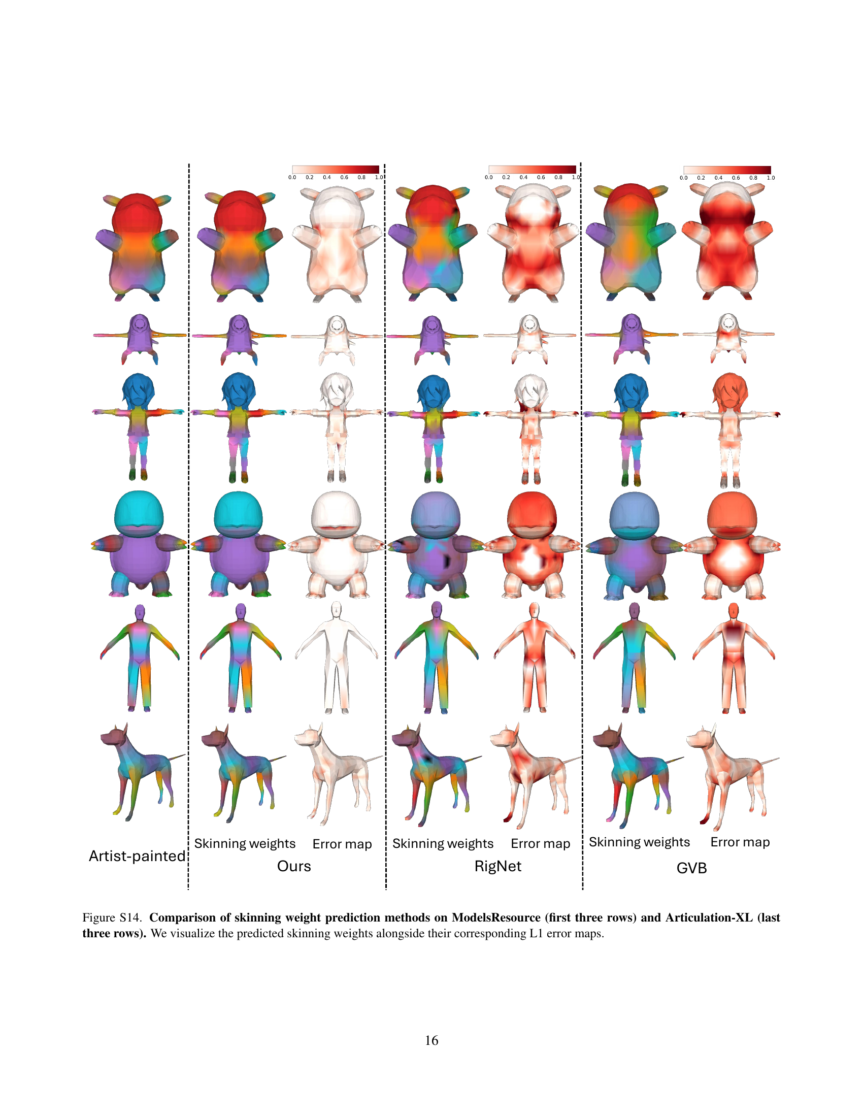
🔼 This figure compares the performance of different skinning weight prediction methods. The top three rows show results from the ModelsResource dataset, and the bottom three rows display results from the Articulation-XL dataset. For each method (Ours, RigNet, GVB), the figure visualizes both the predicted skinning weights and their corresponding L1 error maps, enabling a direct comparison of accuracy. The error maps highlight discrepancies between predicted and ground truth weights, indicating areas where the method’s performance is better or worse.
read the caption
Figure S14: Comparison of skinning weight prediction methods on ModelsResource (first three rows) and Articulation-XL (last three rows). We visualize the predicted skinning weights alongside their corresponding L1 error maps.

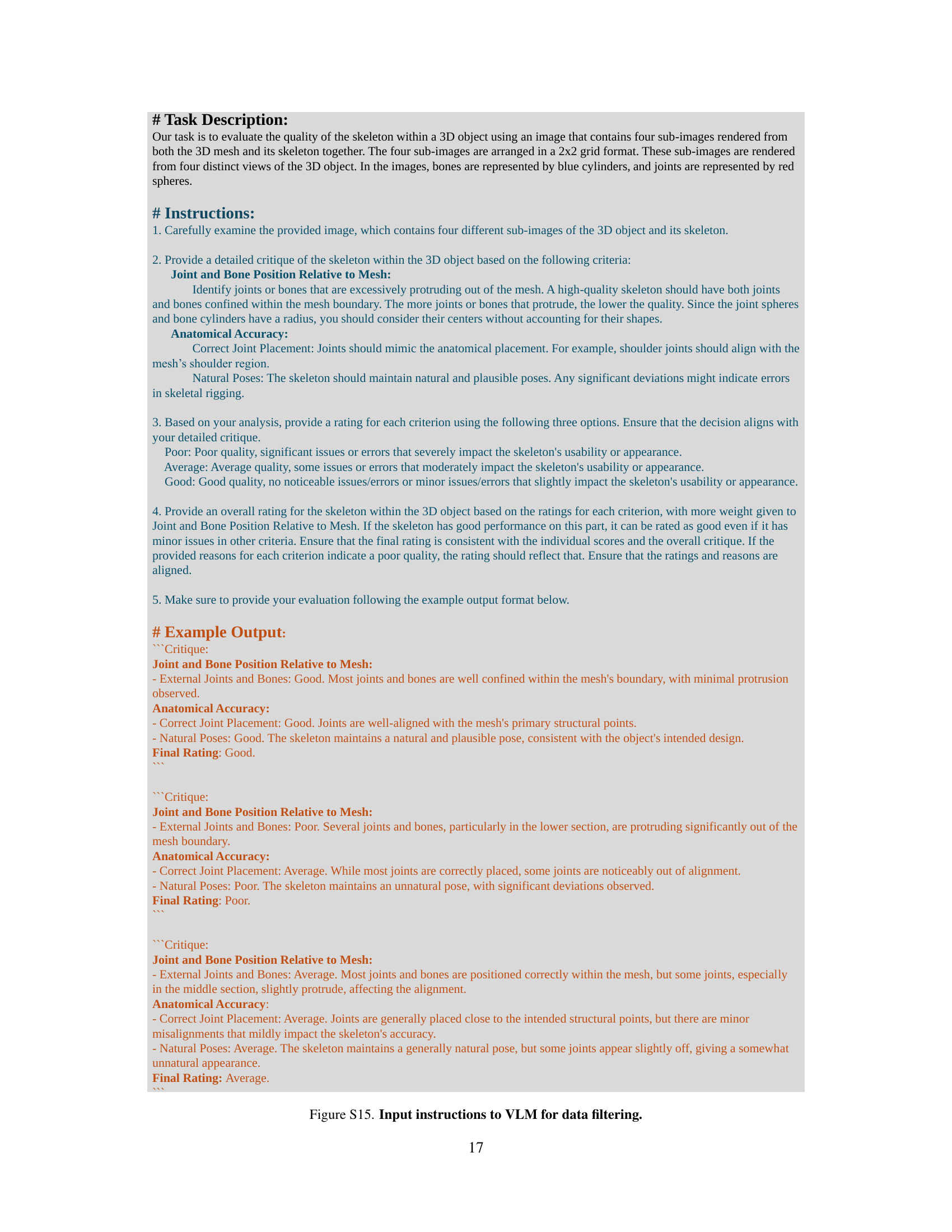
🔼 This figure shows the detailed instructions given to the Vision-Language Model (VLM) for the task of data filtering. The instructions guide the VLM on how to assess the quality of a skeleton within a 3D model using four rendered views of both the 3D mesh and the skeleton. The VLM evaluates based on criteria like whether joints and bones extend beyond the mesh’s boundaries and how well the skeleton’s pose aligns with the model’s anatomy. The instructions also outline a three-point rating system (Poor, Average, Good) and provide example evaluations demonstrating the process.
read the caption
Figure S15: Input instructions to VLM for data filtering.

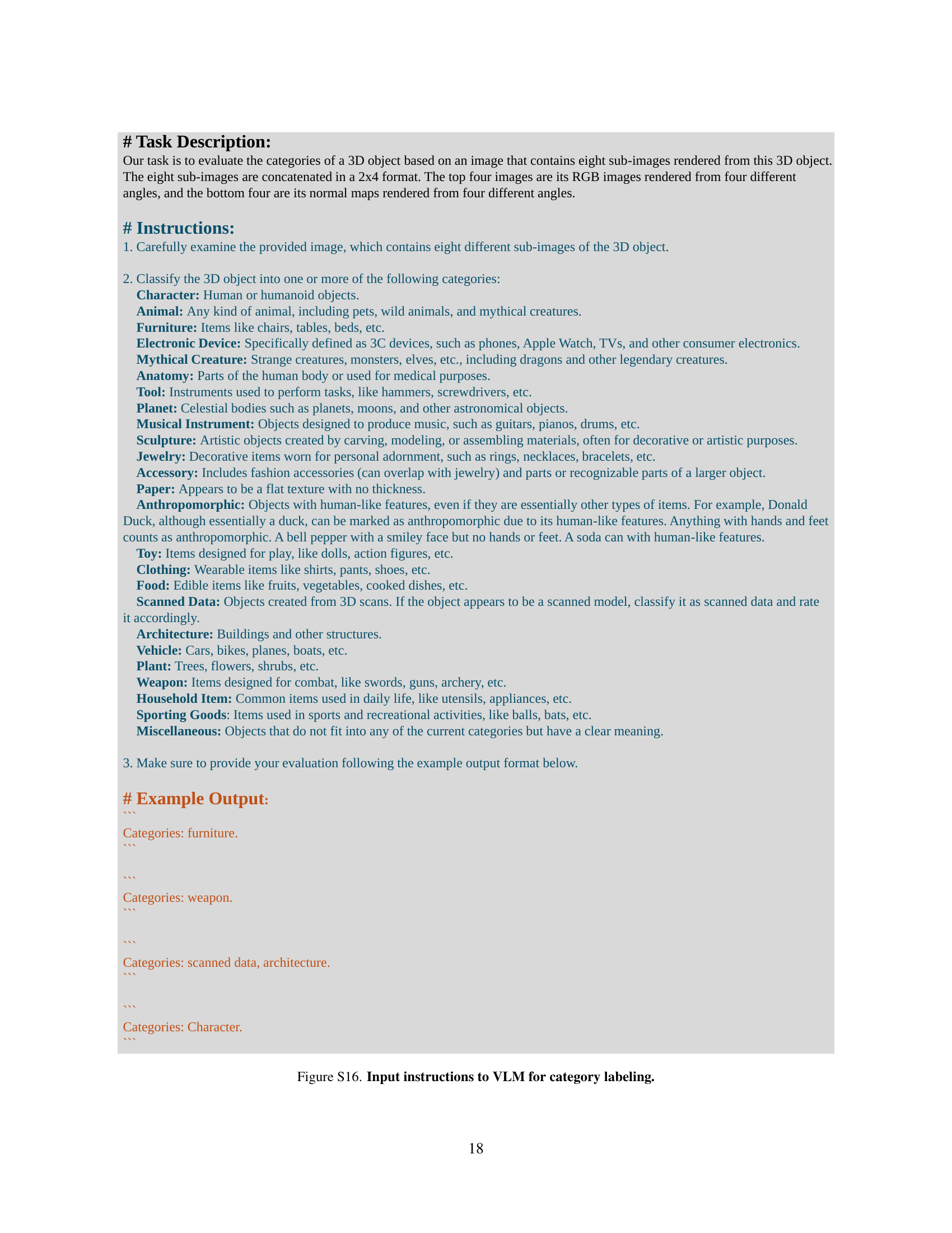
🔼 The figure shows the detailed instructions given to the Vision-Language Model (VLM) for the task of automatically assigning categories to 3D objects. The instructions emphasize the importance of carefully examining eight sub-images of each 3D object (four RGB images and four normal maps, each from a different angle) before assigning categories. A comprehensive list of categories is provided, including character, animal, furniture, electronic device, mythical creature, anatomy, tool, planet, musical instrument, sculpture, jewelry, accessory, paper, anthropomorphic object, toy, clothing, food, scanned data, architecture, vehicle, plant, weapon, household item, and miscellaneous. The instructions also include an example of the expected output format.
read the caption
Figure S16: Input instructions to VLM for category labeling.

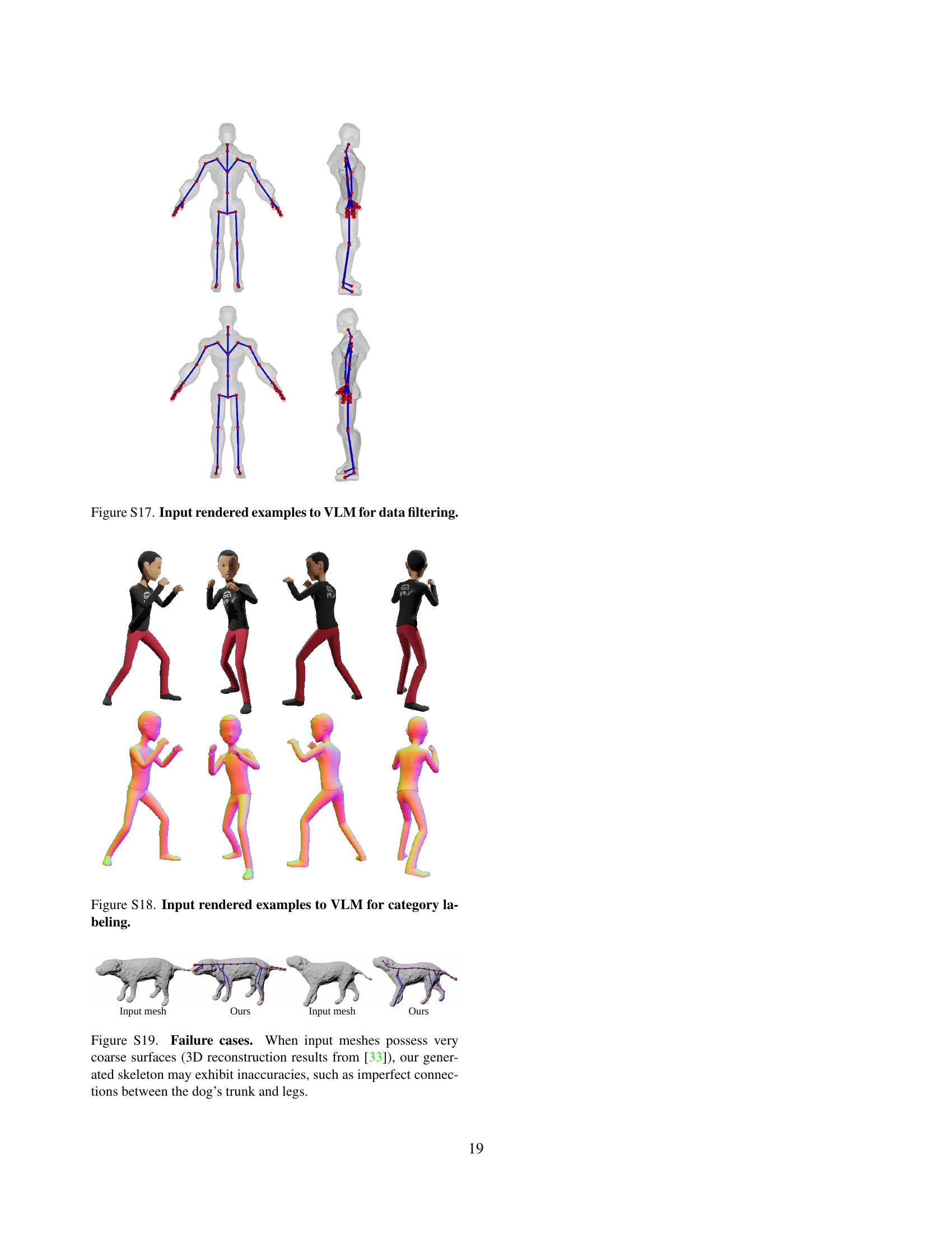
🔼 This figure shows example images used to train a Vision-Language Model (VLM) for filtering low-quality 3D models and skeletons from the dataset. The images consist of four views of the same 3D object, rendered with its skeleton. The VLM is trained to assess the quality of the skeleton based on its alignment with the mesh and its overall anatomical plausibility. This process ensures that only high-quality articulation data is used for training the MagicArticulate model.
read the caption
Figure S17: Input rendered examples to VLM for data filtering.

🔼 This figure shows example images used to train a Vision-Language Model (VLM) for automatically assigning category labels to 3D models in the Articulation-XL dataset. Each image contains eight sub-images: four RGB images and four corresponding normal maps, each from a different viewpoint. These images serve as input to the VLM, which learns to associate visual features with specific object categories.
read the caption
Figure S18: Input rendered examples to VLM for category labeling.
More on tables
| Dataset | Precision | Recall | avg L1 | |
|---|---|---|---|---|
| GVB | ModelsResource | 69.3% | 79.2% | 0.687 |
| RigNet | 77.1% | 83.5% | 0.464 | |
| Ours | 82.1% | 81.6% | 0.398 | |
| GVB | Articulation-XL | 75.7% | 68.3% | 0.724 |
| RigNet | 72.4% | 71.1% | 0.698 | |
| Ours | 80.7% | 77.2% | 0.337 |
🔼 This table presents a quantitative comparison of skinning weight prediction performance between three methods: the proposed method, Geodesic Voxel Binding (GVB), and RigNet. The comparison uses three metrics: Precision, Recall, and the average L1-norm error. Higher precision and recall values indicate better performance in accurately identifying the influence of joints on vertices. A lower average L1-norm error signifies better accuracy in predicting the skinning weights themselves.
read the caption
Table 2: Quantitative comparison on skinning weight prediction. We compare our method with GVB and RigNet. For Precision and Recall, larger values indicate better performance. For average L1-norm error, smaller values are preferred.
| CD-J2J | CD-J2B | CD-B2B | |
|---|---|---|---|
| w/o data filtering | 2.982 | 2.327 | 2.015 |
| 4,096 points | 2.635 | 2.024 | 1.727 |
| 12,288 points | 2.685 | 2.048 | 1.760 |
| Ours (8,192) | 2.586 | 1.959 | 1.661 |
🔼 This table presents the results of ablation studies conducted on the skeleton generation aspect of the MagicArticulate model. It shows how different choices in the model’s design impact its performance. Specifically, it examines the effect of data filtering, and the number of sampled points used as input, on the model’s accuracy in generating skeletons for 3D models. The performance is evaluated using three Chamfer Distance metrics: CD-J2J, CD-J2B, and CD-B2B, measuring the distances between the generated skeleton and ground truth skeleton joints and bones. Lower values indicate better performance.
read the caption
Table 3: Ablation studies for skeleton generation.
| Precision | Recall | avg L1 | |
|---|---|---|---|
| w/o geodesic dist. | 81.5% | 77.7% | 0.444 |
| w/o weights norm | 82.0% | 77.9% | 0.436 |
| w/o shape features | 81.4% | 81.3% | 0.412 |
| Ours | 82.1% | 81.6% | 0.398 |
🔼 This table presents the results of ablation studies conducted to evaluate the impact of different components within the skinning weight prediction framework. It shows how the performance metrics (Precision, Recall, and average L1) change when specific components are removed or altered, thus revealing the contribution of each component to the overall accuracy of the skinning weight prediction.
read the caption
Table 4: Ablation studies on skinning weight prediction.
| Dataset | Precision | Recall | avg L1 | avg Dist. | |
|---|---|---|---|---|---|
| GVB | ModelsResource | 69.3% | 79.2% | 0.687 | 0.0067 |
| RigNet | 77.1% | 83.5% | 0.464 | 0.0054 | |
| Ours | 82.1% | 81.6% | 0.398 | 0.0039 | |
| GVB | Articulation-XL | 75.7% | 68.3% | 0.724 | 0.0095 |
| RigNet | 72.4% | 71.1% | 0.698 | 0.0091 | |
| Ours | 80.7% | 77.2% | 0.337 | 0.0050 |
🔼 Table S5 presents a quantitative comparison of skinning weight prediction methods, specifically comparing the proposed method against Geodesic Voxel Binding (GVB) and RigNet. The evaluation metrics include precision, recall (higher values are better), average L1-norm error, and average distance error (lower values are better). This allows for a comprehensive assessment of the accuracy and effectiveness of each method in predicting skinning weights.
read the caption
Table S5: Quantitative comparison on skinning weight prediction. We compare our method with GVB and RigNet. For Precision and Recall, larger values indicate better performance. For average L1-norm error and average distance error, smaller values are preferred.
| Precision | Recall | avg L1 | avg Dist. | |
|---|---|---|---|---|
| w/o geodesic dist. | 81.5% | 77.7% | 0.444 | 0.0046 |
| w/o weights norm | 82.0% | 77.9% | 0.436 | 0.0045 |
| w/o shape features | 81.4% | 81.3% | 0.412 | 0.0042 |
| Ours | 82.1% | 81.6% | 0.398 | 0.0039 |
🔼 This table presents the results of ablation studies conducted on the ModelsResource dataset to evaluate the impact of different components on skinning weight prediction. The ablation studies remove or modify key parts of the proposed method (e.g., geodesic distance, weight normalization, shape features) to isolate their contribution to the overall prediction accuracy. The table shows the precision, recall, average L1-norm error, and average distance error for each ablation experiment, allowing for a quantitative analysis of the importance of each component.
read the caption
Table S6: Ablation studies on ModelsResource for skinning weight prediction.
| Category | # Objects | Category | # Objects | Category | # Objects |
|---|---|---|---|---|---|
| character | 16020 | miscellaneous | 584 | architecture | 132 |
| anthropomorphic | 13393 | scanned data | 546 | planet | 49 |
| animal | 4760 | plant | 382 | paper | 46 |
| mythical creature | 4734 | accessories | 293 | musical instrument | 25 |
| toy | 1360 | vehicle | 283 | sporting goods | 21 |
| weapon | 1257 | sculpture | 276 | armor | 13 |
| anatomy | 1227 | household items | 274 | robot | 4 |
| clothing | 595 | food | 206 |
🔼 This table presents a detailed breakdown of the object categories included in the Articulation-XL dataset. It shows the number of 3D models belonging to each category, providing a quantitative overview of the dataset’s composition and diversity across various object types.
read the caption
Table S7: Object counts for each category in the Articulation-XL dataset.
Full paper#