The snake in the Brownian sphere

↗ arXiv ↗ Hugging Face

TL;DR

#

Key Takeaways

#

Why does it matter?

#

This paper is important because it establishes a fundamental link between the Brownian sphere and the Brownian snake. The methods in this study can potentially extend to other Brownian surfaces, offering new perspectives on random geometry and its connections to quantum gravity.

Visual Insights

#

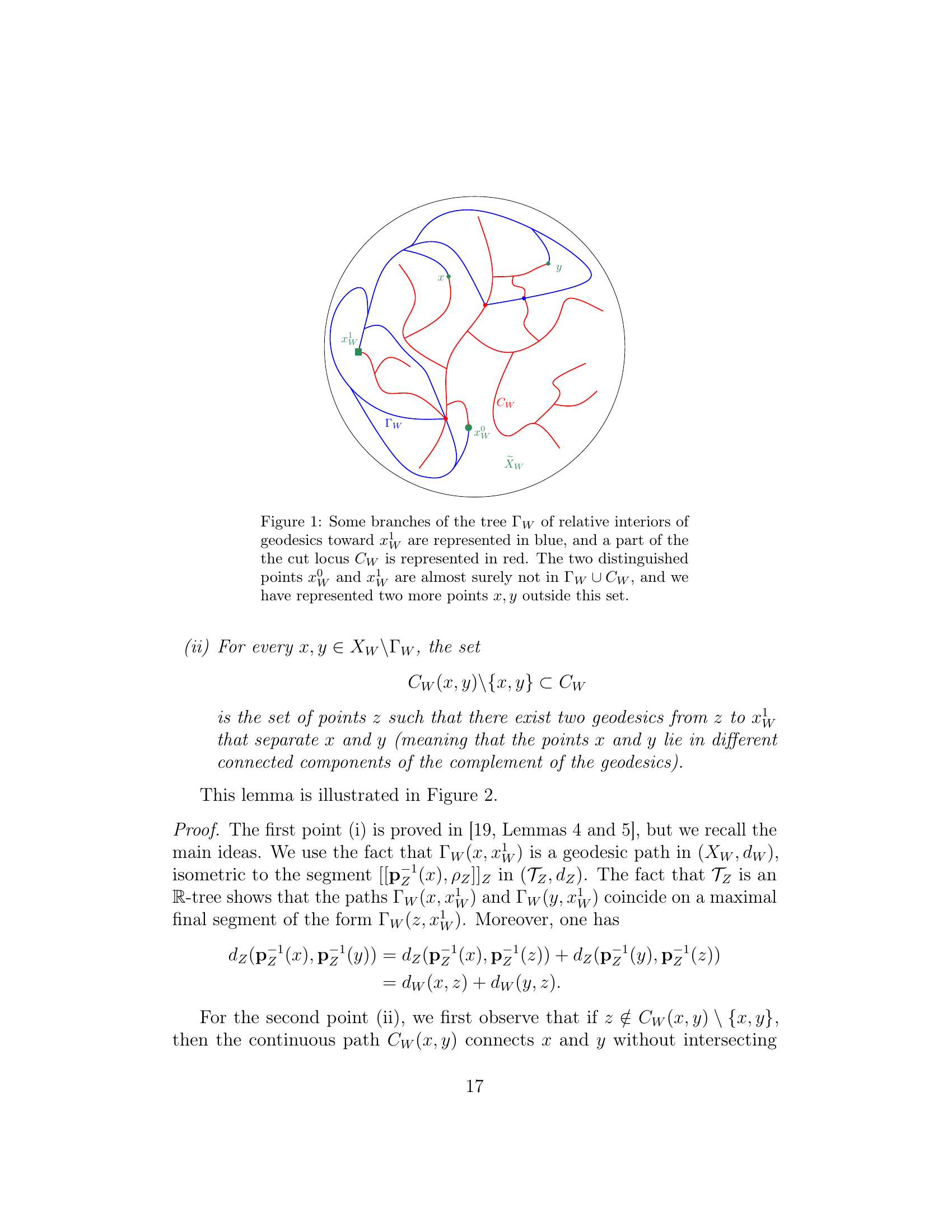
🔼 The figure illustrates key components of the Brownian sphere, highlighting the relationship between the Brownian tree and the sphere’s geometry. Specifically, it shows the cut locus (in red), which is the set of points in the sphere with multiple shortest paths to a reference point (xW⁰), and the relative interiors of geodesics (in blue), which are paths in the tree that connect to the reference point. The two distinguished points (xW⁰ and xW¹), along with two additional points (x and y), are also shown to illustrate the relationships. This visualization aids in understanding the inverse continuum CVS mapping process.

read the caption

Figure 1: Some branches of the tree ΓWsubscriptΓ𝑊\Gamma_{W}roman_Γ start_POSTSUBSCRIPT italic_W end_POSTSUBSCRIPT of relative interiors of geodesics toward xW1superscriptsubscript𝑥𝑊1x_{W}^{1}italic_x start_POSTSUBSCRIPT italic_W end_POSTSUBSCRIPT start_POSTSUPERSCRIPT 1 end_POSTSUPERSCRIPT are represented in blue, and a part of the the cut locus CWsubscript𝐶𝑊C_{W}italic_C start_POSTSUBSCRIPT italic_W end_POSTSUBSCRIPT is represented in red. The two distinguished points xW0superscriptsubscript𝑥𝑊0x_{W}^{0}italic_x start_POSTSUBSCRIPT italic_W end_POSTSUBSCRIPT start_POSTSUPERSCRIPT 0 end_POSTSUPERSCRIPT and xW1superscriptsubscript𝑥𝑊1x_{W}^{1}italic_x start_POSTSUBSCRIPT italic_W end_POSTSUBSCRIPT start_POSTSUPERSCRIPT 1 end_POSTSUPERSCRIPT are almost surely not in ΓW∪CWsubscriptΓ𝑊subscript𝐶𝑊\Gamma_{W}\cup C_{W}roman_Γ start_POSTSUBSCRIPT italic_W end_POSTSUBSCRIPT ∪ italic_C start_POSTSUBSCRIPT italic_W end_POSTSUBSCRIPT, and we have represented two more points x,y𝑥𝑦x,yitalic_x , italic_y outside this set.

In-depth insights

#

Brownian Snake

#

The “Brownian snake” refers to a continuous Markov process that encodes the trajectory of a labeled tree. This process arises as the limit of discrete snake-like explorations on random trees, mirroring how Brownian motion arises from random walks. The snake’s head, represented by a process Z indexed by the tree’s contour, carries the Brownian label. The lifetime process is denoted as ’e’. In the context of the Brownian sphere, the Brownian snake plays a fundamental role in inverting the CVS bijection, which maps between random trees with labels and random metric spaces homeomorphic to the sphere. The snake’s properties, particularly its continuous path and the independent increments of its labels along disjoint paths in the tree, are crucial for reconstructing the underlying tree structure from the sphere’s metric.

CVS Inverse Map

#

The paper delves into inverting the continuous Cori-Vauquelin-Schaeffer (CVS) bijection, a crucial step in understanding the relationship between random trees and the Brownian sphere. The inverse map aims to reconstruct the Brownian snake, the core element in the sphere’s construction, directly from the sphere itself. Constructing the inverse is challenging because the CVS bijection is not injective, requiring the introduction of an orientation to resolve ambiguities. The approach uses the cut locus of a point on the Brownian sphere and constructs an R-tree whose Brownian labels represent the snake. Measurability issues are handled carefully, ensuring the inverse map is well-defined. The inverse function hinges on recovering an orientation parameter, along with utilizing geometric features like cut loci to reconstruct tree structures and their labels.

Orientation Choice

#

The orientation choice in the context of the Brownian sphere is a subtle but crucial aspect. Unlike smooth manifolds where standard definitions of orientation readily apply, the Brownian sphere, arising as a scaling limit of random planar maps, presents challenges due to its singular nature. Previous works often circumvented explicit discussion of orientation, yet it plays a significant role in inverting the CVS bijection. The paper highlights that there are two possible orientations for the Brownian sphere, reversing which corresponds to reflecting the CRT. The authors propose addressing this by considering the Brownian sphere as a metric space and assigning a random orientation based on a variable, accounting for the two possibilities. This approach introduces measurability issues that need careful handling, contrasting with defining the Brownian sphere directly as an oriented metric space, which would necessitate revisiting existing constructions. Ultimately, handling the orientation is vital for constructing a measurable inverse of the CVS bijection.

CRT Recovery

#

While the input text doesn’t explicitly have a ‘CRT Recovery’ section, inferring from the context, it would likely discuss how to reconstruct the Continuum Random Tree (CRT) from the Brownian sphere. It may involve inverting the CVS bijection. Key aspects would involve using the cut locus and understanding the roles of the marked points and orientation. The recovery process would need to measurably map features of the Brownian sphere (distances, area measure) back to the tree structure and Brownian labels of the snake. The challenge lies in dealing with the non-uniqueness due to orientation and ensuring measurability of the inverse mapping, and the use of metric measure space to achieve that.

Measure’s Role

#

The paper emphasizes the crucial role of the area measure (μ) in characterizing the Brownian sphere. While the metric structure (d) largely defines the sphere, the area measure provides additional information, enabling a more complete description. Le Gall’s work [15] indicates that the measure is almost surely determined by the metric. The paper also explores the connection between the Gromov-Hausdorff space and the measure by defining mappings and emphasizing that these are invariant under the specific isometries used, and that the measure could be defined using them. This hints at a deeper interplay between metric and measure, suggesting that measure-theoretic properties are intrinsic to the geometric structure of the Brownian sphere and can be characterized by the geometry.

More visual insights

#

More on figures

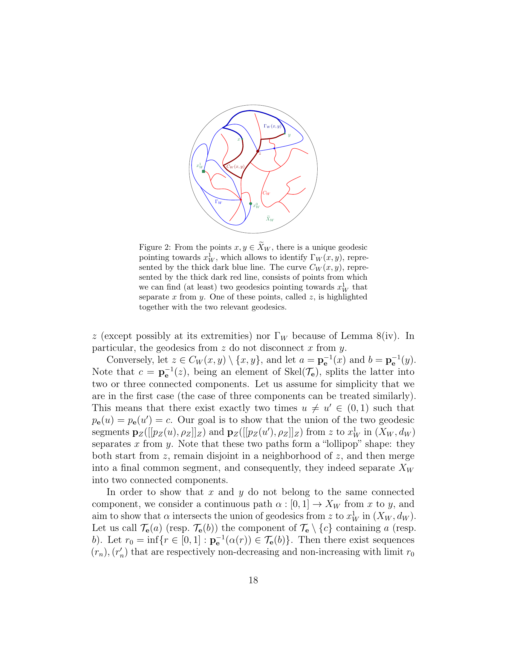
🔼 Figure 2 illustrates key properties of the Brownian sphere. Two points, x and y, are selected outside of the cut locus (Cw) and the set of relative interiors of geodesics to x¹w (Fw). A unique geodesic connects each point to x¹w. The union of these geodesics up to their intersection at a point z is represented by a thick blue line and denoted as Γw(x, y). The thick red curve Cw(x, y) shows the set of points that have at least two geodesics connecting them to x¹w and that these geodesics separate x from y. Point z is highlighted to emphasize its role in this separation.

read the caption

Figure 2: From the points x,y∈X~W𝑥𝑦subscript~𝑋𝑊x,y\in\widetilde{X}_{W}italic_x , italic_y ∈ over~ start_ARG italic_X end_ARG start_POSTSUBSCRIPT italic_W end_POSTSUBSCRIPT, there is a unique geodesic pointing towards xW1subscriptsuperscript𝑥1𝑊x^{1}_{W}italic_x start_POSTSUPERSCRIPT 1 end_POSTSUPERSCRIPT start_POSTSUBSCRIPT italic_W end_POSTSUBSCRIPT, which allows to identify ΓW⁢(x,y)subscriptΓ𝑊𝑥𝑦\Gamma_{W}(x,y)roman_Γ start_POSTSUBSCRIPT italic_W end_POSTSUBSCRIPT ( italic_x , italic_y ), represented by the thick dark blue line. The curve CW⁢(x,y)subscript𝐶𝑊𝑥𝑦C_{W}(x,y)italic_C start_POSTSUBSCRIPT italic_W end_POSTSUBSCRIPT ( italic_x , italic_y ), represented by the thick dark red line, consists of points from which we can find (at least) two geodesics pointing towards xW1subscriptsuperscript𝑥1𝑊x^{1}_{W}italic_x start_POSTSUPERSCRIPT 1 end_POSTSUPERSCRIPT start_POSTSUBSCRIPT italic_W end_POSTSUBSCRIPT that separate x𝑥xitalic_x from y𝑦yitalic_y. One of these points, called z𝑧zitalic_z, is highlighted together with the two relevant geodesics.

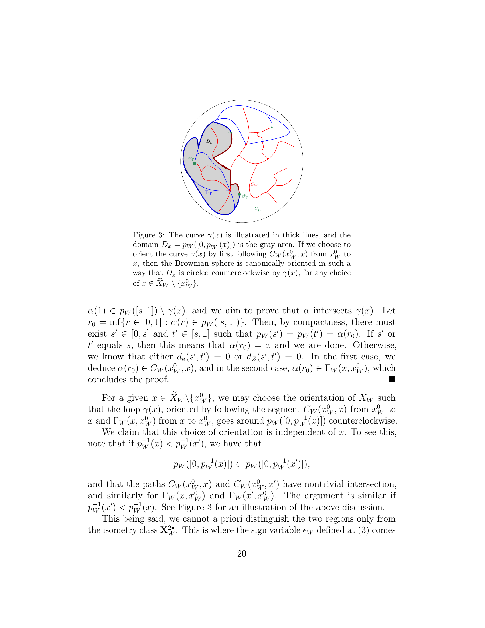
🔼 Figure 3 illustrates how the Brownian sphere is canonically oriented using a simple closed loop γ(x), formed by the union of two geodesics. The loop γ(x) separates the sphere into two regions, Dx and its complement. The orientation is determined such that the loop circles Dx counterclockwise, based on a specific ordering of the geodesics, ensuring a consistent orientation regardless of the choice of point x. The gray shaded area represents Dx.

read the caption

Figure 3: The curve γ⁢(x)𝛾𝑥\gamma(x)italic_γ ( italic_x ) is illustrated in thick lines, and the domain Dx=pW⁢([0,pW−1⁢(x)])subscript𝐷𝑥subscript𝑝𝑊0superscriptsubscript𝑝𝑊1𝑥D_{x}=p_{W}([0,p_{W}^{-1}(x)])italic_D start_POSTSUBSCRIPT italic_x end_POSTSUBSCRIPT = italic_p start_POSTSUBSCRIPT italic_W end_POSTSUBSCRIPT ( [ 0 , italic_p start_POSTSUBSCRIPT italic_W end_POSTSUBSCRIPT start_POSTSUPERSCRIPT - 1 end_POSTSUPERSCRIPT ( italic_x ) ] ) is the gray area. If we choose to orient the curve γ⁢(x)𝛾𝑥\gamma(x)italic_γ ( italic_x ) by first following CW⁢(xW0,x)subscript𝐶𝑊superscriptsubscript𝑥𝑊0𝑥C_{W}(x_{W}^{0},x)italic_C start_POSTSUBSCRIPT italic_W end_POSTSUBSCRIPT ( italic_x start_POSTSUBSCRIPT italic_W end_POSTSUBSCRIPT start_POSTSUPERSCRIPT 0 end_POSTSUPERSCRIPT , italic_x ) from xW0superscriptsubscript𝑥𝑊0x_{W}^{0}italic_x start_POSTSUBSCRIPT italic_W end_POSTSUBSCRIPT start_POSTSUPERSCRIPT 0 end_POSTSUPERSCRIPT to x𝑥xitalic_x, then the Brownian sphere is canonically oriented in such a way that Dxsubscript𝐷𝑥D_{x}italic_D start_POSTSUBSCRIPT italic_x end_POSTSUBSCRIPT is circled counterclockwise by γ⁢(x)𝛾𝑥\gamma(x)italic_γ ( italic_x ), for any choice of x∈X~W∖{xW0}𝑥subscript~𝑋𝑊superscriptsubscript𝑥𝑊0x\in\widetilde{X}_{W}\setminus\{x_{W}^{0}\}italic_x ∈ over~ start_ARG italic_X end_ARG start_POSTSUBSCRIPT italic_W end_POSTSUBSCRIPT ∖ { italic_x start_POSTSUBSCRIPT italic_W end_POSTSUBSCRIPT start_POSTSUPERSCRIPT 0 end_POSTSUPERSCRIPT }.

Full paper

#