ReQFlow: Rectified Quaternion Flow for Efficient and High-Quality Protein Backbone Generation

2502.14637

Angxiao Yue et el.

🤗 2025-02-24

TL;DR
#

Protein backbone generation is a critical step in de novo protein design. Existing diffusion and flow-based generative models often produce proteins with poor designability and suffer from computational inefficiency. This limits their practical use in large-scale applications. To solve these issues, the paper introduces rectified quaternion flow.

Key Takeaways
#

Why does it matter?
#

This paper introduces ReQFlow, a novel method for generating high-quality protein backbones efficiently. It is important because it addresses the limitations of current generative models, offering faster computation without compromising designability. It opens new avenues for protein design, facilitating the development of novel enzymes and drugs.

Visual Insights
#

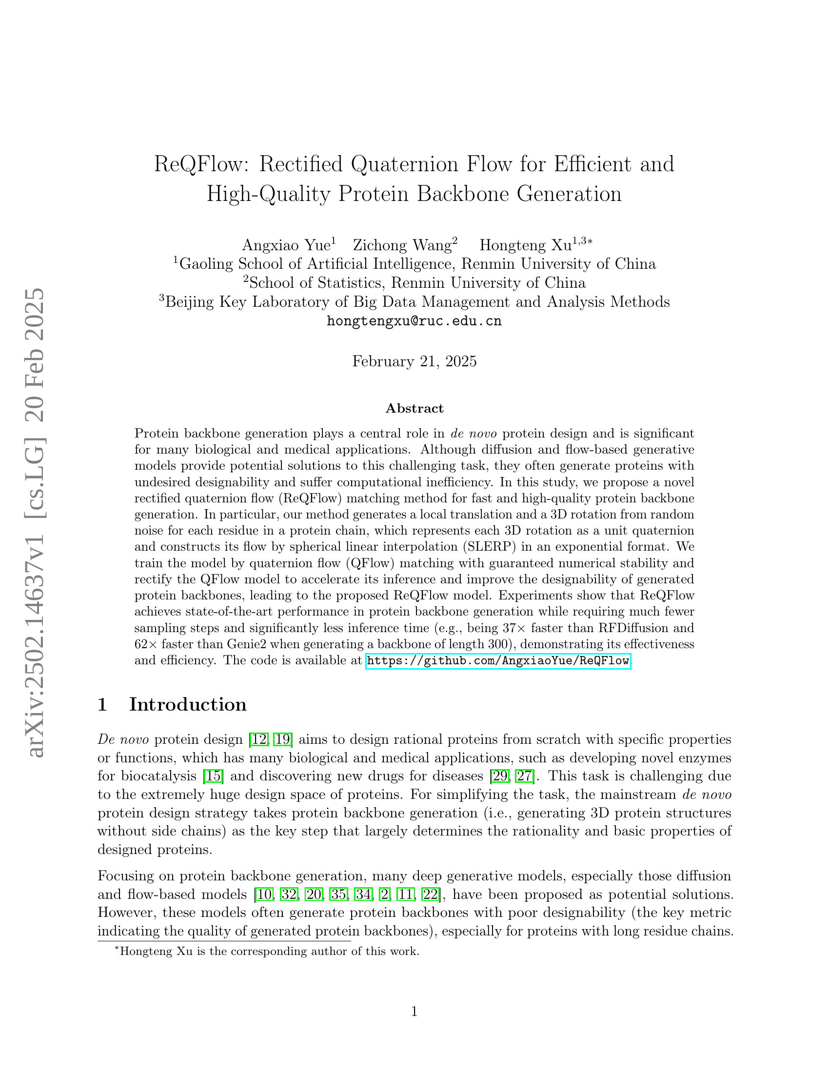
🔼 This figure illustrates the ReQFlow method for protein backbone generation. Each residue in the protein backbone is represented as a frame, which is a rigid transformation in 3D space. This transformation consists of a local 3D translation and a 3D rotation represented as a unit quaternion. The figure shows how random noise is converted into a quaternion flow using spherical linear interpolation (SLERP) to produce a protein backbone. The process involves rectifying the flow to improve designability and efficiency. The final output is a protein backbone.
read the caption
Figure 1: An illustration of our rectified quaternion flow matching method, in which each residue is represented as a frame associated with a local transformation.

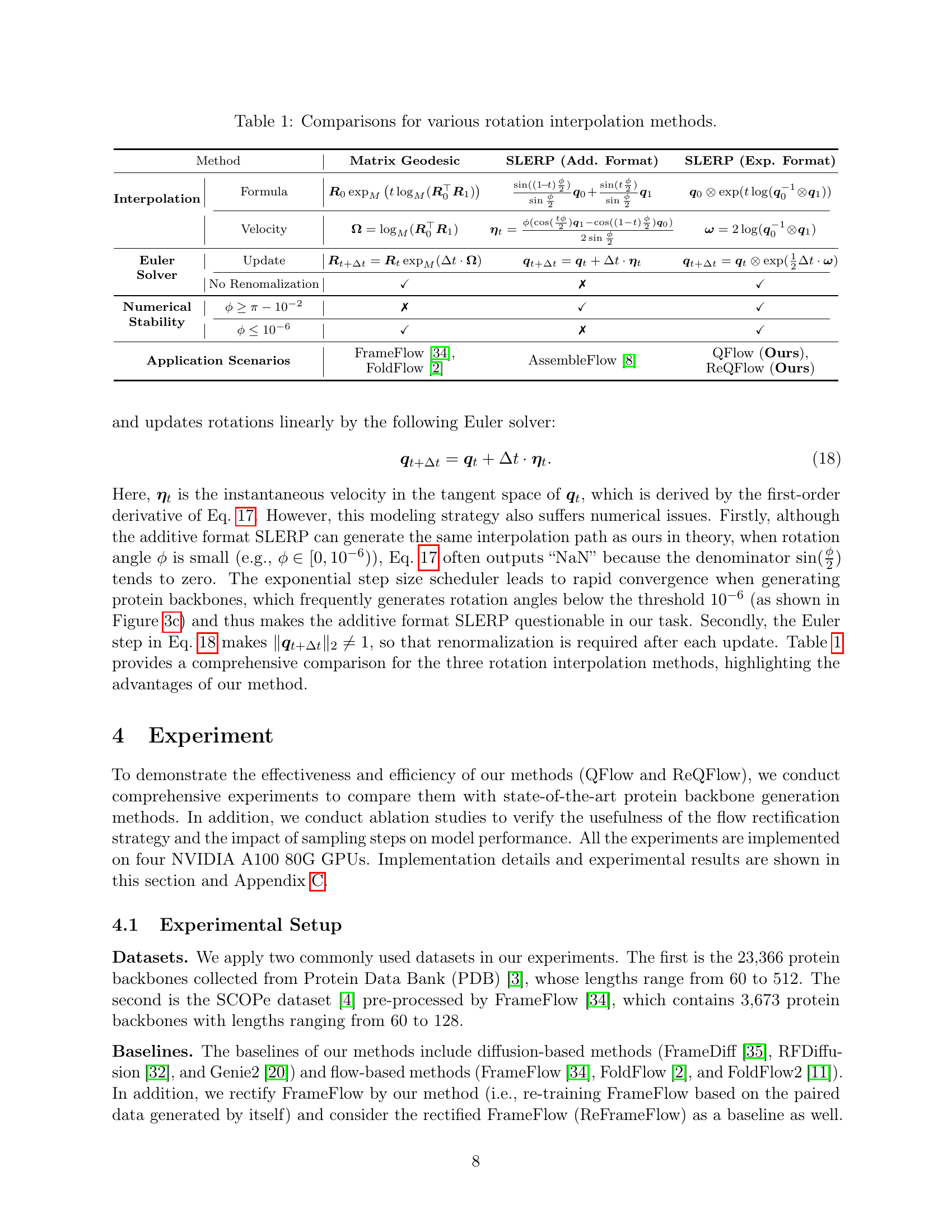
Method		Matrix Geodesic	SLERP (Add. Format)	SLERP (Exp. Format)
Interpolation	Formula	$\bm{R}_{0}\exp_{M}\left(t\log_{M}(\bm{R}_{0}^{\top}\bm{R}_{1})\right)$	$\frac{\sin((1\!-\!t)\frac{\phi}{2})}{\sin\frac{\phi}{2}}\bm{q}_{0}\!+\!\frac{% \sin(t\frac{\phi}{2})}{\sin\frac{\phi}{2}}\bm{q}_{1}$	$\bm{q}_{0}\otimes\exp(t\log(\bm{q}_{0}^{-1}\!\otimes\!\bm{q}_{1}))$
Interpolation	Velocity	$\bm{\Omega}=\log_{M}(\bm{R}_{0}^{\top}\bm{R}_{1})$	$\bm{\eta}_{t}=\frac{\phi(\cos(\frac{t\phi}{2})\bm{q}_{1}-\cos((1-t)\frac{\phi}% {2})\bm{q}_{0})}{2\sin\frac{\phi}{2}}$	$\bm{\omega}=2\log(\bm{q}_{0}^{-1}\!\otimes\!\bm{q}_{1})$
Euler Solver	Update	$\bm{R}_{t+\Delta t}=\bm{R}_{t}\exp_{M}(\Delta t\cdot\bm{\Omega})$	$\bm{q}_{t+\Delta t}=\bm{q}_{t}+\Delta t\cdot\bm{\eta}_{t}$	$\bm{q}_{t+\Delta t}=\bm{q}_{t}\otimes\exp(\frac{1}{2}\Delta t\cdot\bm{\omega})$
Euler Solver	No Renomalization	✓	✗	✓
Numerical Stability	$\phi\geq\pi-10^{-2}$	✗	✓	✓
Numerical Stability	$\phi\leq 10^{-6}$	✓	✗	✓
Application Scenarios		FrameFlow [34], FoldFlow [2]	AssembleFlow [8]	QFlow (Ours), ReQFlow (Ours)

🔼 This table compares different methods for interpolating rotations, a key operation in generating protein backbones. It shows the formula used for each method, the velocity calculation, the type of Euler solver used (if any), whether renormalization is needed, and the numerical stability. It also highlights the methods’ application scenarios in relevant papers. This allows comparison of the methods’ properties and suitability for various applications in protein backbone generation.
read the caption
Table 1: Comparisons for various rotation interpolation methods.

In-depth insights
#

Quaternion Flows
#

Quaternion flows offer a compact, computationally efficient, and gimbal lock-free representation for 3D rotations, crucial in protein backbone generation. Leveraging the exponential SLERP format guarantees numerical stability, particularly advantageous when dealing with large rotation angles, often encountered in protein structures. By training the model with quaternion flow matching, the method ensures consistent effectiveness in generating protein backbones and addresses the limitations of matrix-based approaches prone to numerical instability, enhancing overall efficiency and generation quality.

Rectified Flows
#

Rectified flows, a concept gaining traction in generative modeling, present a compelling approach to enhancing the efficiency and quality of data generation. Unlike traditional generative models that rely on complex iterative processes, rectified flows aim to streamline the transformation from a simple noise distribution to the desired data distribution. This is achieved by learning a smooth, deterministic flow that directly maps noise to data, effectively ‘rectifying’ the initially disordered noise into an organized structure. The core idea is to minimize the distance between the generated samples and the true data distribution, guiding the flow towards a more direct and accurate mapping. This approach holds significant promise for accelerating the generation process, reducing computational costs, and improving the fidelity of generated samples. However, challenges remain in designing effective architectures and training strategies to ensure the flow remains smooth and invertible, particularly for high-dimensional and complex data distributions. Furthermore, exploring the theoretical properties of rectified flows, such as their convergence behavior and generalization capabilities, is crucial for establishing their robustness and reliability.

Protein Design
#

De novo protein design is a powerful tool with biological and medical applications, like novel enzymes or new drugs, but the vast design space poses challenges. The mainstream strategy involves generating protein backbones (3D structures without side chains), as rationality and properties are determined. Deep generative models, such as diffusion and flow-based models, show potential. However, they often produce proteins with poor designability, especially for long residue chains, limiting practical use.

Long Chains
#

The paper tackles the challenge of generating long protein chains, a known issue in protein design. Many existing methods struggle to maintain designability (quality) when the residue count increases. This work seems to address this limitation, potentially by using a novel approach (ReQFlow) that is more robust to the complexities introduced by longer sequences. Overcoming this hurdle is significant as it unlocks the possibility of designing more complex and functional proteins for various applications. This issue is also a crucial element of the generalization ability, because the models are expected to work out of their original size limitations. Based on high-quality data from the start is the most reliable option for producing more accurate results.

Future Protein
#

Future protein research will likely focus on improving generation quality for long-chain proteins through enhanced training datasets, refined model architectures, and pre-training techniques. The goal is to create controllable protein designs for side chain and full-atom generation, expanding applications in diverse fields. Additionaly, computational efficiency of existing models such as ReQFlow has to be enhanced further for practical application.

More visual insights
#

More on figures

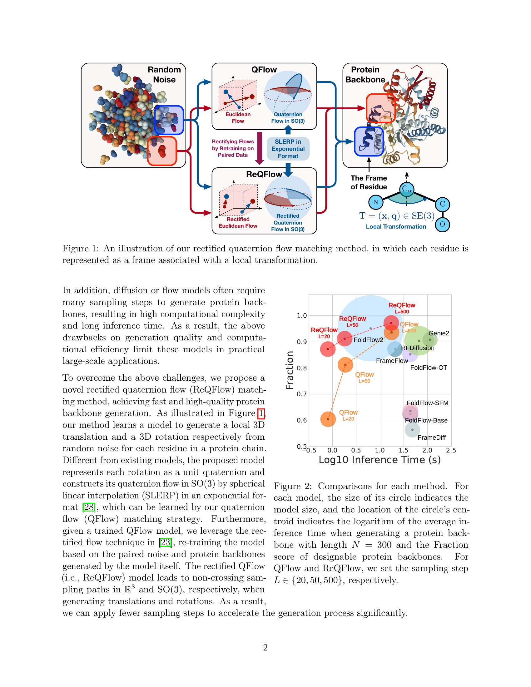
🔼 Figure 2 is a scatter plot visualizing the performance of various protein backbone generation methods. Each method is represented by a circle, with the circle’s size corresponding to the model’s size and its position determined by two factors: average inference time (log scale) and fraction score of successfully generated backbones (designable backbones with scRMSD <2Å) when generating a protein backbone of length 300. Different sampling steps (L) were used for QFlow and ReQFlow (20, 50, and 500 steps), showing the trade-off between speed and quality. This plot helps compare the efficiency and designability of different methods in generating long protein chains.
read the caption
Figure 2: Comparisons for each method. For each model, the size of its circle indicates the model size, and the location of the circle’s centroid indicates the logarithm of the average inference time when generating a protein backbone with length N=300𝑁300N=300italic_N = 300 and the Fraction score of designable protein backbones. For QFlow and ReQFlow, we set the sampling step L∈{20,50,500}𝐿2050500L\in\{20,50,500\}italic_L ∈ { 20 , 50 , 500 }, respectively.

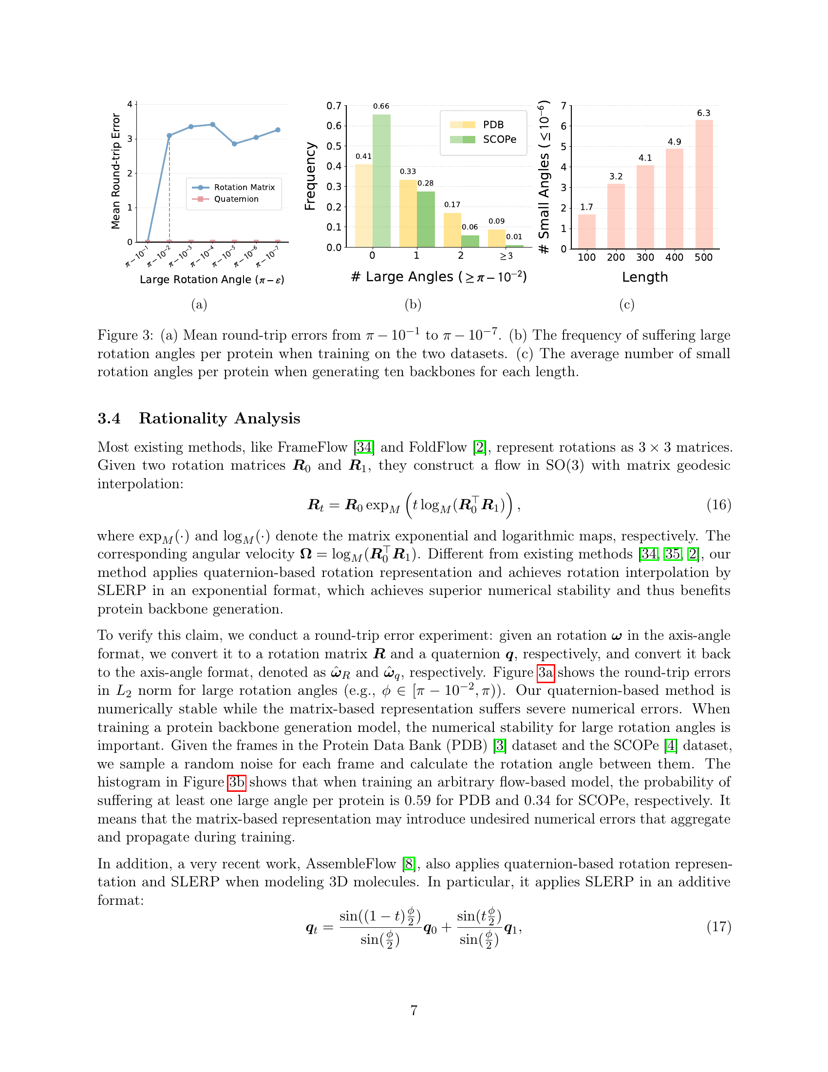
🔼 The figure shows the mean round-trip errors for different rotation angles, ranging from π−10⁻¹ to π−10⁻⁷, comparing two methods: using rotation matrices and using quaternions. The results illustrate the superior numerical stability of the quaternion-based rotation representation, especially for large rotation angles close to π, which is crucial for protein backbone generation models’ accuracy and efficiency.
read the caption
(a)

🔼 The figure shows the frequency of large rotation angles (≥ π - 10⁻²) per protein when training on two datasets: PDB and SCOPe. The x-axis represents the size of the rotation angle, ranging from π - 10⁻¹ to 0, with a logarithmic scale. The y-axis represents the frequency, showing how often a protein in the dataset contains a rotation angle of a given size. The figure illustrates the numerical stability of using quaternions for representing rotations, as the quaternion-based approach is less sensitive to large rotation angles than the matrix-based representation. This is significant because large rotation angles can lead to instability and error in model training.
read the caption
(b)

🔼 This figure visualizes protein backbones generated by ReQFlow for various lengths (100, 200, 300, 400, 500, 600). It showcases the model’s capability to generate high-quality protein backbones of varying lengths, demonstrating its ability to generate longer sequences while maintaining structural integrity.
read the caption
(c)

🔼 This figure demonstrates the numerical stability of using quaternions to represent rotations in protein backbone generation. Panel (a) shows that the mean round-trip error when converting between axis-angle representation and quaternion representation is consistently lower for quaternions, especially for large rotation angles close to π. Panel (b) illustrates the frequency of encountering large rotation angles (close to π) during the training process of protein backbone generation models, which highlights the importance of numerical stability for large rotation angles in practical applications. Panel (c) displays the average number of small rotation angles observed in generated protein backbones, illustrating that the number of small rotation angles increases with the length of the protein backbone. This shows the robustness of the quaternion representation for various backbone length.
read the caption
Figure 3: (a) Mean round-trip errors from π−10−1𝜋superscript101\pi-10^{-1}italic_π - 10 start_POSTSUPERSCRIPT - 1 end_POSTSUPERSCRIPT to π−10−7𝜋superscript107\pi-10^{-7}italic_π - 10 start_POSTSUPERSCRIPT - 7 end_POSTSUPERSCRIPT. (b) The frequency of suffering large rotation angles per protein when training on the two datasets. (c) The average number of small rotation angles per protein when generating ten backbones for each length.

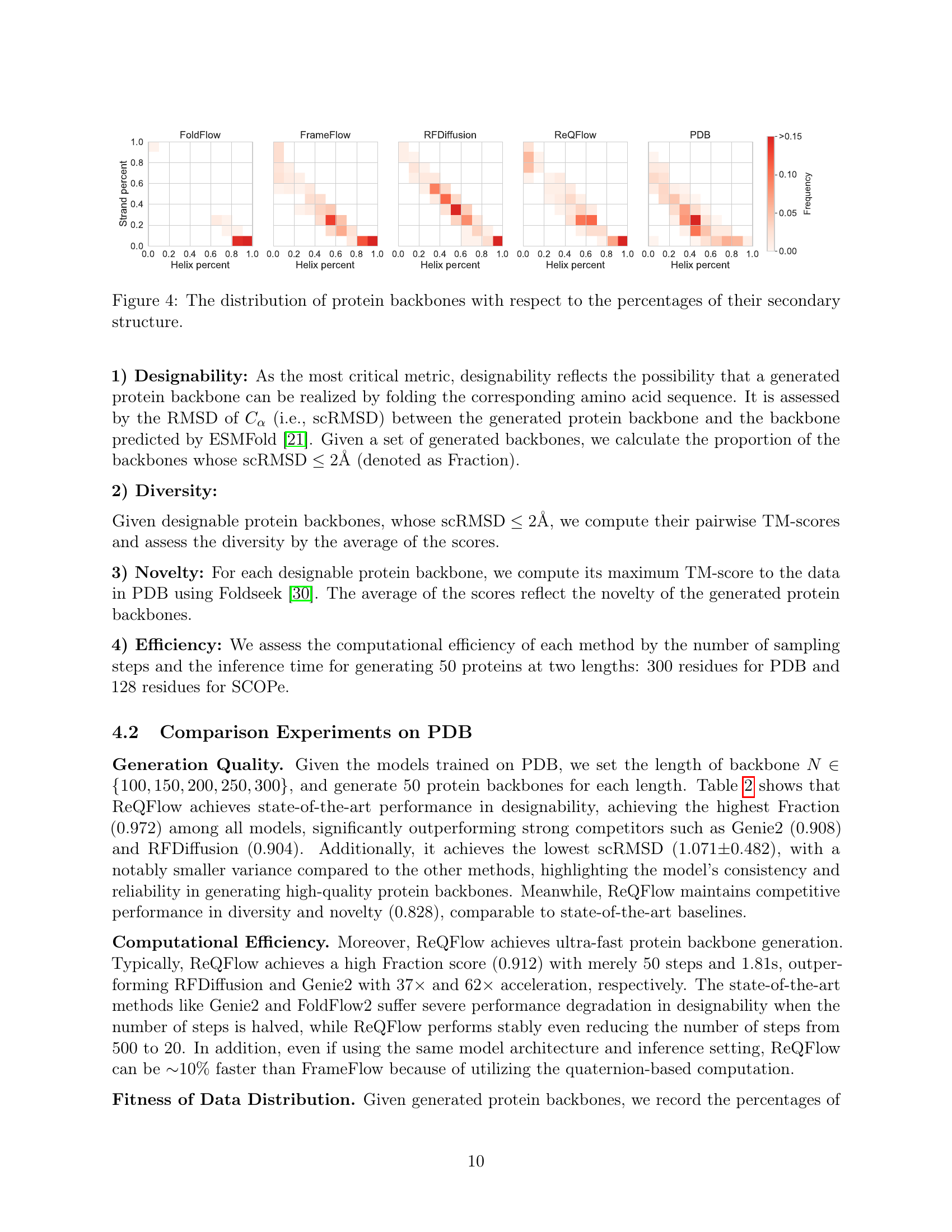
🔼 Figure 4 visualizes the distribution of generated protein backbones concerning the proportions of their secondary structures (helix and strand). It allows for a comparison of the distribution generated by different models (ReQFlow, FrameFlow, RFDiffusion, and FoldFlow) against the distribution observed in the Protein Data Bank (PDB) dataset. The goal is to assess how well the generated backbones match the natural distribution of secondary structures found in real proteins, indicating the models’ ability to capture realistic structural features.
read the caption
Figure 4: The distribution of protein backbones with respect to the percentages of their secondary structure.

🔼 The figure shows the designability of generated protein backbones for various methods across different lengths. Designability, measured by Fraction, represents the proportion of generated backbones with scRMSD (self-consistency RMSD) below 2Å. Higher Fraction indicates better designability. The plot visually compares the performance of different methods in generating designable protein backbones of varying lengths. The x-axis represents the length of the protein backbone, and the y-axis represents the Fraction score indicating designability.
read the caption
(a) Fraction

🔼 The figure shows the self-consistency root mean square deviation (scRMSD) for various protein backbone generation methods across different protein lengths. scRMSD measures the structural similarity between a generated protein backbone and the backbone predicted using a protein structure prediction method. Lower scRMSD values indicate better agreement between the generated and predicted structures, suggesting higher designability of the generated protein backbone. The graph likely displays scRMSD values as a function of protein length, allowing comparison of different methods’ performance in generating accurate and designable backbones across different protein lengths.
read the caption
(b) scRMSD

🔼 This figure shows six protein backbone structures generated by the ReQFlow model. Each structure corresponds to a different length protein: 100, 200, 300, 400, 500, and 600 amino acids. The visualization helps illustrate the model’s capability to generate long chains while maintaining structural integrity.
read the caption
(c) Samples generated by ReQFlow

🔼 Figure 5 presents a comparison of different methods for generating long-chain protein backbones, focusing on their designability. Panel (a) shows the fraction of designable proteins (scRMSD < 2Å) generated by each method as the length of the protein backbone increases. Panel (b) shows the average scRMSD for each method across various protein lengths. Panel (c) provides visual examples of protein backbones generated by ReQFlow for different lengths, illustrating the quality of the generated structures.
read the caption
Figure 5: The comparison for various methods on the designability of generated long-chain protein backbones.

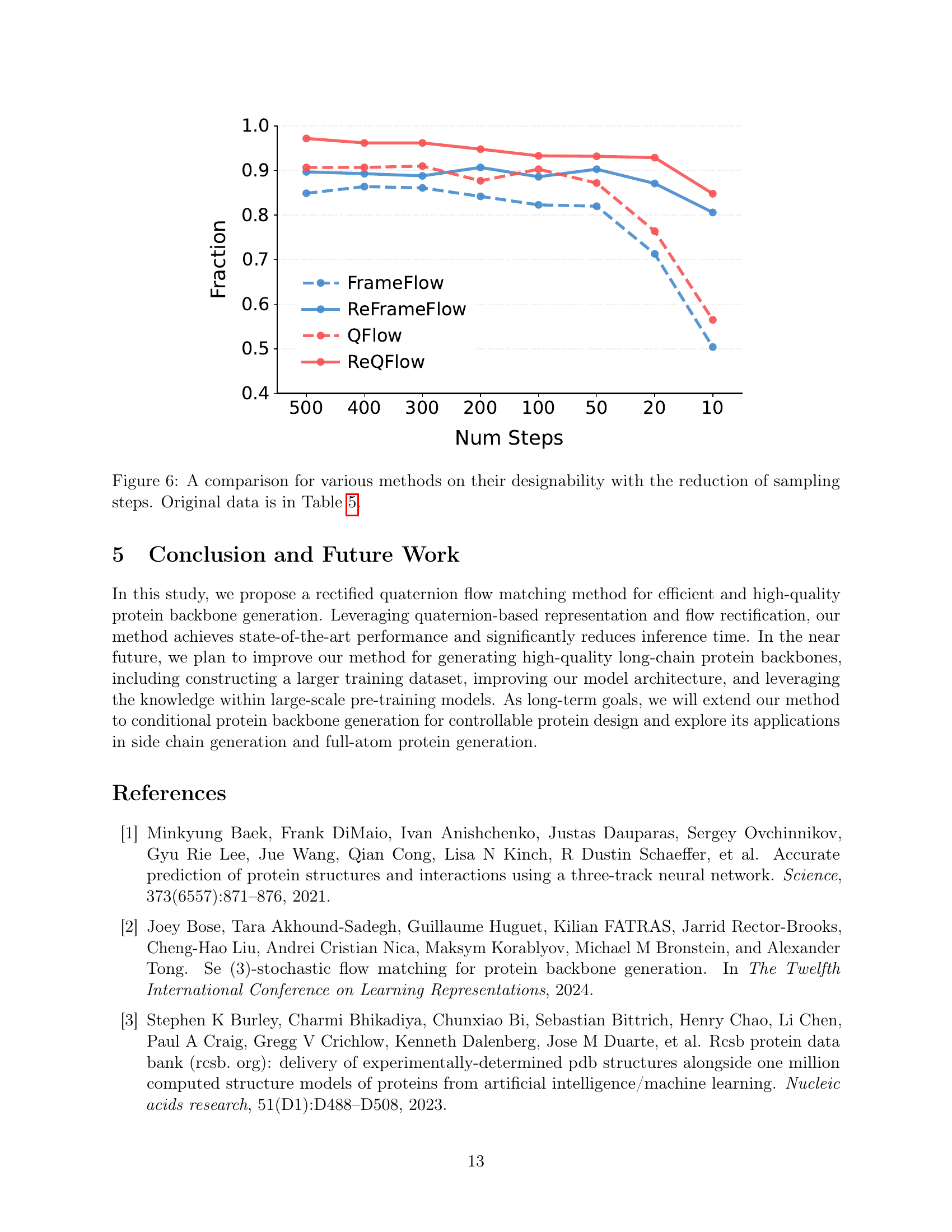
🔼 Figure 6 illustrates the impact of reducing the number of sampling steps on the designability of protein backbones generated by different methods. Designability, a key metric representing the likelihood that a generated backbone can fold into a stable protein structure, is measured as the fraction of backbones with a Ca RMSD (scRMSD) below 2Å from a reference structure. The figure shows that as the number of sampling steps decreases, the designability of protein backbones generated by most methods deteriorates. However, ReQFlow demonstrates superior robustness, maintaining high designability even with significantly fewer sampling steps. This highlights the effectiveness and efficiency of ReQFlow in protein backbone generation. The specific values of Fraction scores are provided in Table 5.
read the caption
Figure 6: A comparison for various methods on their designability with the reduction of sampling steps. Original data is in Table 5.

🔼 This figure shows the distribution of protein lengths in the PDB and SCOPe datasets used for training the model. The x-axis represents the protein length, and the y-axis represents the frequency or count of proteins with that length. Two separate histograms are shown, one for the PDB dataset and one for the SCOPe dataset. The distributions help to illustrate the range of protein lengths present in each dataset and provides context for the model’s performance on proteins of various sizes.
read the caption
Figure 7: The length distribution of PDB and SCOPe dataset we use for training.

More on tables

Method	Efficiency		Designability		Diversity	Novelty
Method	Step	Time(s)	Fraction $\uparrow$	scRMSD $\downarrow$	TM $\downarrow$	TM $\downarrow$
RFDiffusion	50	66.23	0.904	1.102 ${}_{\pm\text{1.617}}$	0.382	0.822
Genie2	1000	112.93	0.908	1.132 ${}_{\pm\text{1.389}}$	0.370	0.759
	500	55.86	0.000	18.169 ${}_{\pm\text{5.963}}$	-	0.115
FrameDiff	500	48.12	0.564	2.936 ${}_{\pm\text{3.093}}$	0.441	0.799
FoldFlow ${}_{\text{Base}}$	500	43.52	0.624	3.080 ${}_{\pm\text{3.449}}$	0.469	0.870
FoldFlow ${}_{\text{SFM}}$	500	43.63	0.636	3.031 ${}_{\pm\text{3.589}}$	0.411	0.848
FoldFlow ${}_{\text{OT}}$	500	43.35	0.852	1.760 ${}_{\pm\text{2.593}}$	0.434	0.857
FoldFlow2	50	6.35	0.952	1.083 ${}_{\pm\text{1.308}}$	0.373	0.813
	20	2.63	0.644	3.060 ${}_{\pm\text{3.210}}$	0.339	0.736
FrameFlow	500	20.72	0.872	1.380 ${}_{\pm\text{1.392}}$	0.346	0.803
	200	8.69	0.864	1.542 ${}_{\pm\text{1.889}}$	0.348	0.809
	100	4.20	0.708	2.167 ${}_{\pm\text{2.373}}$	0.332	0.806
	50	2.23	0.704	2.639 ${}_{\pm\text{3.079}}$	0.334	0.791
	20	0.84	0.436	4.652 ${}_{\pm\text{4.390}}$	0.319	0.772
	10	0.47	0.180	7.343 ${}_{\pm\text{5.125}}$	0.317	0.762
QFlow	500	17.52	0.936	1.163 ${}_{\pm\text{0.938}}$	0.356	0.821
	200	6.85	0.864	1.400 ${}_{\pm\text{1.259}}$	0.344	0.807
	100	3.45	0.916	1.342 ${}_{\pm\text{1.364}}$	0.348	0.809
	50	1.87	0.812	1.785 ${}_{\pm\text{2.151}}$	0.344	0.784
	20	0.81	0.604	3.090 ${}_{\pm\text{3.374}}$	0.325	0.758
	10	0.45	0.332	5.032 ${}_{\pm\text{4.303}}$	0.313	0.715
ReQFlow	500	17.29	0.972	1.071 ${}_{\pm\text{0.482}}$	0.377	0.828
	200	7.44	0.932	1.160 ${}_{\pm\text{0.782}}$	0.384	0.826
	100	3.62	0.928	1.245 ${}_{\pm\text{1.059}}$	0.369	0.819
	50	1.81	0.912	1.254 ${}_{\pm\text{0.915}}$	0.369	0.810
	20	0.80	0.872	1.418 ${}_{\pm\text{0.998}}$	0.355	0.791
	10	0.45	0.676	2.443 ${}_{\pm\text{2.382}}$	0.337	0.760

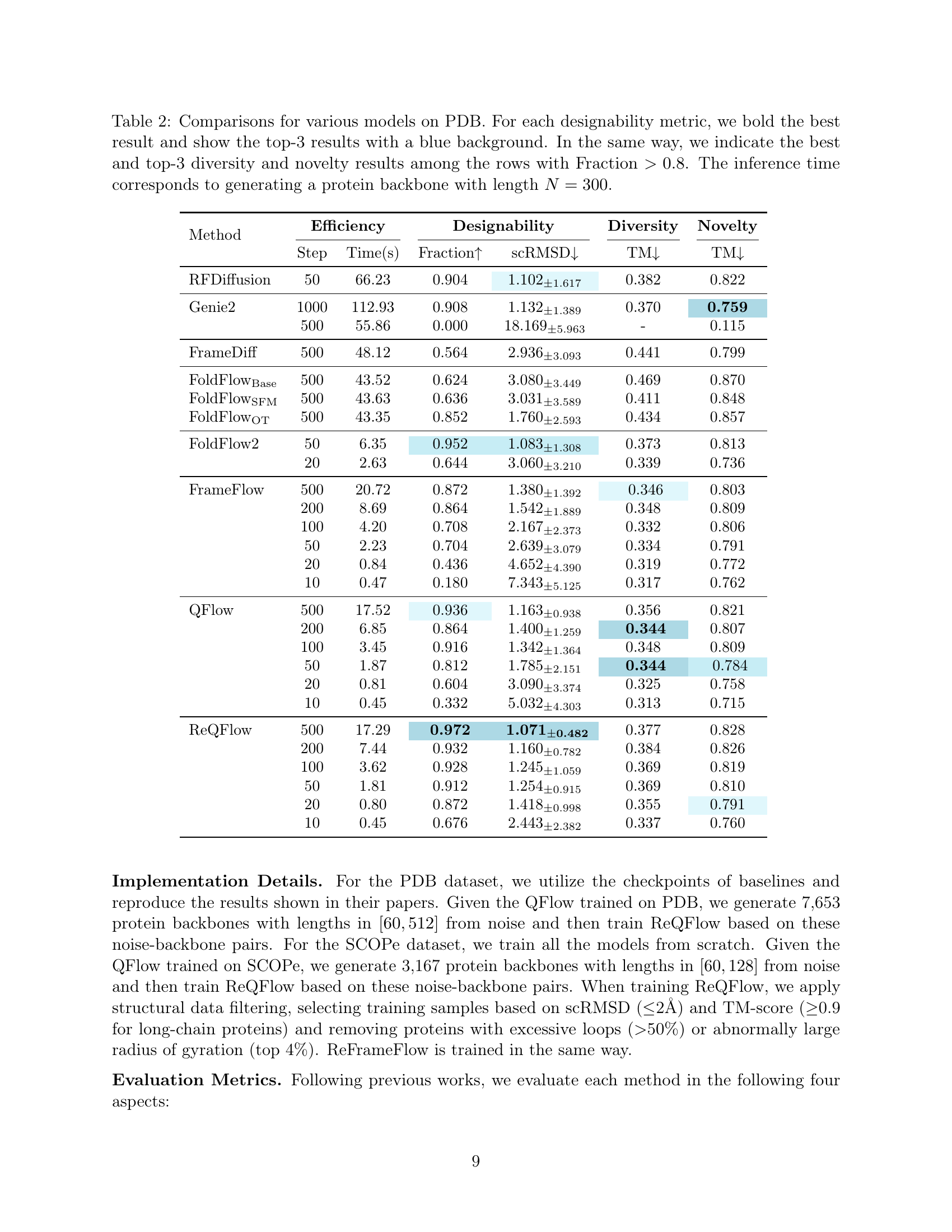
🔼 Table 2 presents a comparison of various protein backbone generation models on the PDB dataset. The table evaluates models based on several key metrics: efficiency (inference time and number of sampling steps), designability (Fraction score and scRMSD), diversity (TM score), and novelty (maximum TM-score to PDB). For each metric, the best-performing models are highlighted in bold, with the top three models for each metric indicated by a blue background. The focus on models with a Fraction score above 0.8 is to highlight the models that generate high-quality backbones (those with high designability, meaning the generated backbone is likely to be produced from a real protein). Inference time is standardized to a backbone length of 300 residues for fair comparison.
read the caption
Table 2: Comparisons for various models on PDB. For each designability metric, we bold the best result and show the top-3 results with a blue background. In the same way, we indicate the best and top-3 diversity and novelty results among the rows with Fraction >0.8absent0.8>0.8> 0.8. The inference time corresponds to generating a protein backbone with length N=300𝑁300N=300italic_N = 300.

Exponential	Flow	Data	Sampling Steps
Scheduler	Rectification	Filtering	500	50	10
✗	✗	✗	0.040	0.004	0.004
✓	✗	✗	0.936	0.812	0.332
✓	✓	✗	0.716	0.704	0.624
✓	✓	✓	0.972	0.912	0.676

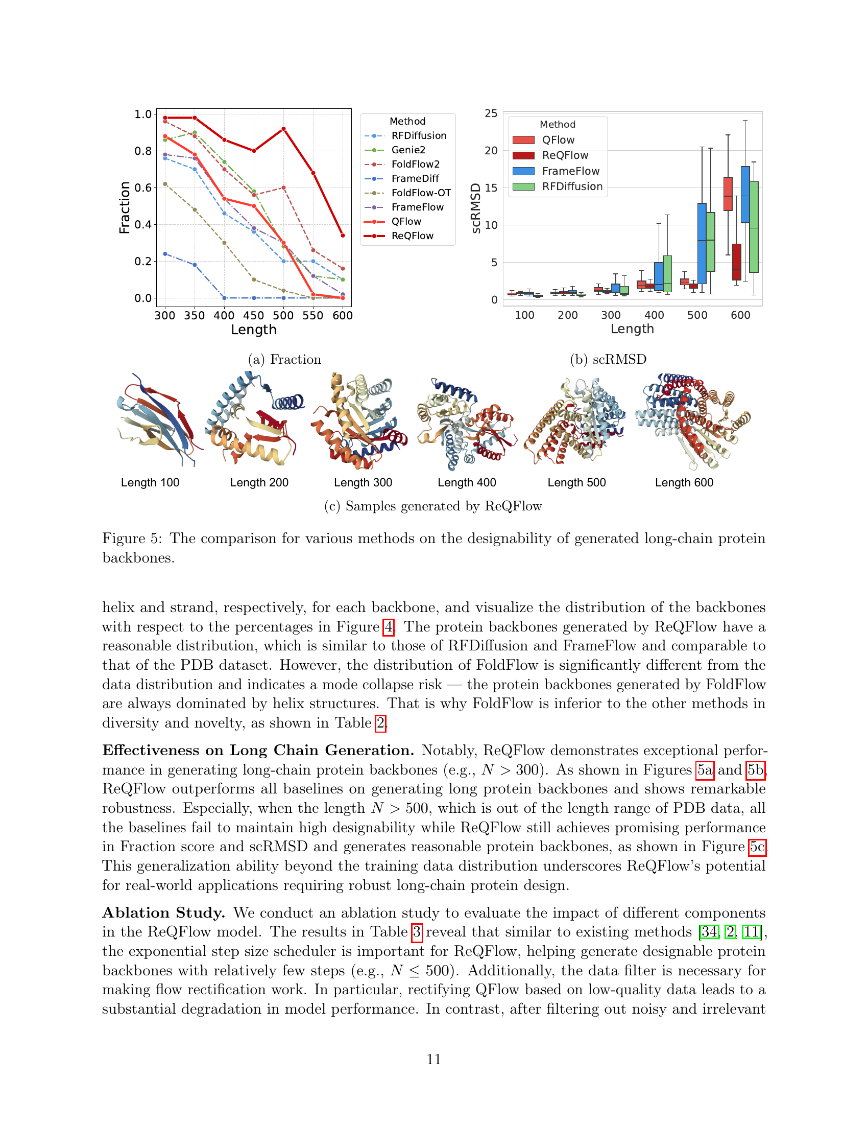
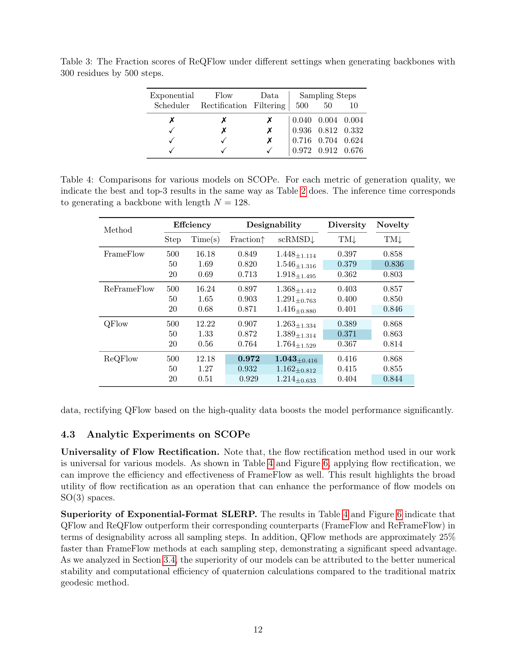
🔼 This table shows the impact of different settings on the performance of the ReQFlow model. Specifically, it shows how using an exponential scheduler, applying flow rectification, and filtering noisy data affect the fraction of designable protein backbones generated, with a fixed backbone length of 300 residues and 500 sampling steps. This helps to understand the relative contributions of each model component.
read the caption
Table 3: The Fraction scores of ReQFlow under different settings when generating backbones with 300 residues by 500 steps.

Method	Effciency		Designability		Diversity	Novelty
Method	Step	Time(s)	Fraction $\uparrow$	scRMSD $\downarrow$	TM $\downarrow$	TM $\downarrow$
FrameFlow	500	16.18	0.849	1.448 ${}_{\pm\text{1.114}}$	0.397	0.858
	50	1.69	0.820	1.546 ${}_{\pm\text{1.316}}$	0.379	0.836
	20	0.69	0.713	1.918 ${}_{\pm\text{1.495}}$	0.362	0.803
ReFrameFlow	500	16.24	0.897	1.368 ${}_{\pm\text{1.412}}$	0.403	0.857
	50	1.65	0.903	1.291 ${}_{\pm\text{0.763}}$	0.400	0.850
	20	0.68	0.871	1.416 ${}_{\pm\text{0.880}}$	0.401	0.846
QFlow	500	12.22	0.907	1.263 ${}_{\pm\text{1.334}}$	0.389	0.868
	50	1.33	0.872	1.389 ${}_{\pm\text{1.314}}$	0.371	0.863
	20	0.56	0.764	1.764 ${}_{\pm\text{1.529}}$	0.367	0.814
ReQFlow	500	12.18	0.972	1.043 ${}_{\pm\text{0.416}}$	0.416	0.868
	50	1.27	0.932	1.162 ${}_{\pm\text{0.812}}$	0.415	0.855
	20	0.51	0.929	1.214 ${}_{\pm\text{0.633}}$	0.404	0.844

🔼 Table 4 presents a comparison of various protein backbone generation models’ performance on the SCOPe dataset. The metrics evaluated include efficiency (measured by the number of steps and inference time), designability (using Fraction score and scRMSD), diversity (using TM-score), and novelty (using TM-score). The best and top 3 results for each metric are highlighted to facilitate comparison. All results are for generating a protein backbone of length N=128. This table allows for a direct comparison of the different models’ performance based on key metrics, highlighting the strengths and weaknesses of each approach in generating high-quality protein structures within this specific dataset.
read the caption
Table 4: Comparisons for various models on SCOPe. For each metric of generation quality, we indicate the best and top-3 results in the same way as Table 2 does. The inference time corresponds to generating a backbone with length N=128𝑁128N=128italic_N = 128.

	Effciency		Designability		Diversity	Novelty	Sec. Struct.
	Step	Time(s)	Fraction $\uparrow$	scRMSD $\downarrow$	TM $\downarrow$	TM $\downarrow$	Helix	Strand
Scope Dataset		-	-	-	-	-	0.330	0.260
FrameFlow	500	16.18	0.849	1.448 ( $\pm$ 1.114)	0.397	0.858 ( $\pm$ 0.059)	0.439	0.236
	400	13.43	0.864	1.353 ( $\pm$ 0.890)	0.380	0.859 ( $\pm$ 0.067)	0.452	0.229
	300	9.80	0.861	1.422 ( $\pm$ 1.178)	0.383	0.870 ( $\pm$ 0.062)	0.449	0.230
	200	6.61	0.842	1.496 ( $\pm$ 1.411)	0.378	0.854 ( $\pm$ 0.062)	0.437	0.237
	100	3.19	0.823	1.517 ( $\pm$ 1.228)	0.378	0.848 ( $\pm$ 0.061)	0.426	0.238
	50	1.69	0.820	1.546 ( $\pm$ 1.316)	0.379	0.836 ( $\pm$ 0.064)	0.441	0.228
	20	0.69	0.713	1.918 ( $\pm$ 1.495)	0.362	0.803 ( $\pm$ 0.071)	0.416	0.219
	10	0.35	0.504	2.924 ( $\pm$ 2.362)	0.344	0.782 ( $\pm$ 0.084)	0.363	0.213
ReFrameFlow	500	16.24	0.897	1.368 ( $\pm$ 1.412)	0.403	0.857 ( $\pm$ 0.052)	0.501	0.187
	400	13.29	0.893	1.328 ( $\pm$ 0.763)	0.402	0.858 ( $\pm$ 0.052)	0.489	0.202
	300	10.27	0.888	1.313 ( $\pm$ 0.686)	0.401	0.860 ( $\pm$ 0.047)	0.485	0.199
	200	6.60	0.907	1.326 ( $\pm$ 0.761)	0.403	0.852 ( $\pm$ 0.051)	0.482	0.206
	100	3.65	0.886	1.322 ( $\pm$ 0.804)	0.408	0.853 ( $\pm$ 0.057)	0.499	0.201
	50	1.65	0.903	1.291 ( $\pm$ 0.763)	0.400	0.850 ( $\pm$ 0.053)	0.504	0.202
	20	0.68	0.871	1.416 ( $\pm$ 0.880)	0.401	0.846 ( $\pm$ 0.050)	0.528	0.190
	10	0.33	0.806	1.696 ( $\pm$ 1.093)	0.390	0.814 ( $\pm$ 0.056)	0.496	0.192
QFlow	500	12.22	0.907	1.263 ( $\pm$ 1.334)	0.389	0.868 ( $\pm$ 0.057)	0.498	0.214
	400	10.11	0.907	1.199 ( $\pm$ 0.847)	0.390	0.873 ( $\pm$ 0.060)	0.476	0.223
	300	7.25	0.910	1.243 ( $\pm$ 1.027)	0.393	0.876 ( $\pm$ 0.056)	0.503	0.209
	200	4.78	0.877	1.309 ( $\pm$ 1.208)	0.389	0.864 ( $\pm$ 0.068)	0.481	0.224
	100	2.48	0.903	1.283 ( $\pm$ 1.027)	0.385	0.884 ( $\pm$ 0.052)	0.476	0.225
	50	1.33	0.872	1.389 ( $\pm$ 1.314)	0.371	0.863 ( $\pm$ 0.064)	0.491	0.206
	20	0.56	0.764	1.764 ( $\pm$ 1.529)	0.367	0.814 ( $\pm$ 0.071)	0.492	0.192
	10	0.29	0.565	2.589 ( $\pm$ 2.216)	0.348	0.772( $\pm$ 0.081)	0.467	0.167
ReQFlow	500	12.18	0.972	1.043 ( $\pm$ 0.416)	0.416	0.868 ( $\pm$ 0.046)	0.507	0.228
	400	10.01	0.962	1.050 ( $\pm$ 0.445)	0.416	0.864 ( $\pm$ 0.053)	0.523	0.212
	300	7.13	0.962	1.076 ( $\pm$ 0.518)	0.415	0.864 ( $\pm$ 0.050)	0.498	0.233
	200	4.80	0.948	1.084 ( $\pm$ 0.509)	0.406	0.862 ( $\pm$ 0.050)	0.513	0.218
	100	2.43	0.933	1.123 ( $\pm$ 0.669)	0.420	0.861 ( $\pm$ 0.053)	0.514	0.310
	50	1.27	0.932	1.162 ( $\pm$ 0.812)	0.415	0.855 ( $\pm$ 0.053)	0.491	0.237
	20	0.51	0.929	1.214 ( $\pm$ 0.633)	0.404	0.844 ( $\pm$ 0.053)	0.514	0.307
	10	0.26	0.848	1.546 ( $\pm$ 0.944)	0.403	0.827 ( $\pm$ 0.058)	0.518	0.195

🔼 Table 5 presents a comprehensive evaluation of various methods for protein backbone generation. It focuses on the performance across different protein lengths, specifically ranging from 60 to 128 amino acids. For each length, ten protein backbones were generated using each method. The table then assesses these generated backbones using several key metrics, including efficiency (steps and time), designability (Fraction, scRMSD), diversity (TM), novelty (TM), and secondary structure content (Helix, Strand). The best and top-three performing methods are highlighted for each metric to allow for easy comparison. This allows for a detailed analysis of each method’s strengths and weaknesses in generating protein backbones of various sizes.
read the caption
Table 5: Unconditional protein backbone generation performance for 10 samples each length in {60,61,⋯,128}6061⋯128\{60,61,\cdots,128\}{ 60 , 61 , ⋯ , 128 }. We report the metrics from Section 2 and we indicate the best and top-3 results in the same way as Table 2 does.

Model	Training Dataset Size	Model Size (M)
RFDiffusion	$>$ 208K	59.8
Genie2	590K	15.7
FrameDiff	23K	16.7
FoldFlow(Base,OT,SFM)	23K	17.5
FoldFlow2	$\sim$ 160K	672
FrameFlow	23K	16.7
QFlow	23K	16.7
ReQFlow	23K+7K	16.7

🔼 This table presents a comparison of different protein backbone generation models in terms of their model size (in millions of parameters) and the size of the training dataset used to train each model (in thousands of samples). It shows that model size and training data size vary considerably across different models, with some models using significantly larger datasets and having substantially more parameters than others. This information is useful to understand the computational cost and resource requirements for training these different models.
read the caption
Table 6: Model Sizes and Training Dataset Sizes

Length $N$	300	350	400	450	500	550	600
RFDiffusion	0.76	0.70	0.46	0.36	0.20	0.20	0.10
Genie2	0.86	0.90	0.74	0.58	0.28	0.12	0.10
FoldFlow2	0.96	0.88	0.70	0.56	0.60	0.26	0.16
FrameDiff	0.24	0.18	0.00	0.00	0.00	0.00	0.00
FoldFlow-OT	0.62	0.48	0.30	0.10	0.04	0.00	0.00
FrameFlow	0.78	0.76	0.54	0.38	0.30	0.12	0.02
QFlow	0.88	0.78	0.54	0.50	0.30	0.02	0.00
ReQFlow	0.98	0.98	0.86	0.80	0.92	0.68	0.34

🔼 Table 7 presents a comparison of various protein backbone generation methods’ performance, specifically focusing on the ‘Fraction Score,’ a metric indicating the proportion of successfully generated backbones meeting a specific designability criterion (scRMSD < 2Å). The table evaluates methods across different backbone lengths, ranging from 300 to 600 amino acid residues. For each length, 50 backbones were generated per method. The best-performing method for each length is highlighted in bold, with the top three best-performing methods for each length shown with a blue background. This allows for a direct comparison of the success rate of each method in producing high-quality, designable protein backbones of varying lengths.
read the caption
Table 7: Comparisions for various methods on their performance (Fraction Score) in long backbone generation. The lengths of the generated backbones range from 300 to 600. We generate 50 samples for each length. We bold the best result and show the top-3 results with a blue background.

TL;DR#

Key Takeaways#

Why does it matter?#

Visual Insights#

In-depth insights#

Quaternion Flows#

Rectified Flows#

Protein Design#

Long Chains#

Future Protein#

More visual insights#

Full paper#