TL;DR#
Sampling in diffusion models is slow, limiting real-world use. Recent methods distill multi-step models into one-step generators, matching distributions with reverse Kullback-Leibler (KL) divergence, which is mode-seeking. This can ignore diverse modes. This paper tackles this by introducing a novel f-divergence minimization framework, called f-distill. It covers divergences with different trade-offs in mode coverage and training variance.
The method derives f-divergence gradients between teacher and student distributions, expressed as score difference and a weighting function based on density ratio. It naturally emphasizes samples with higher teacher density. f-distill outperforms variational score distillation across image tasks using forward-KL and Jensen-Shannon divergences. Jensen-Shannon divergence achieves SOTA one-step generation on ImageNet64 and MS-COCO.
Key Takeaways#
Why does it matter?#
This paper introduces f-distill, a novel framework to enhance one-step diffusion models by minimizing f-divergences, improving image generation quality and diversity. The novel weighting scheme and comprehensive analysis provide insights and opportunities for future research in generative modeling and diffusion-based techniques. The experiments show new SOTA results in ImageNet64 and MS-COCO.
Visual Insights#

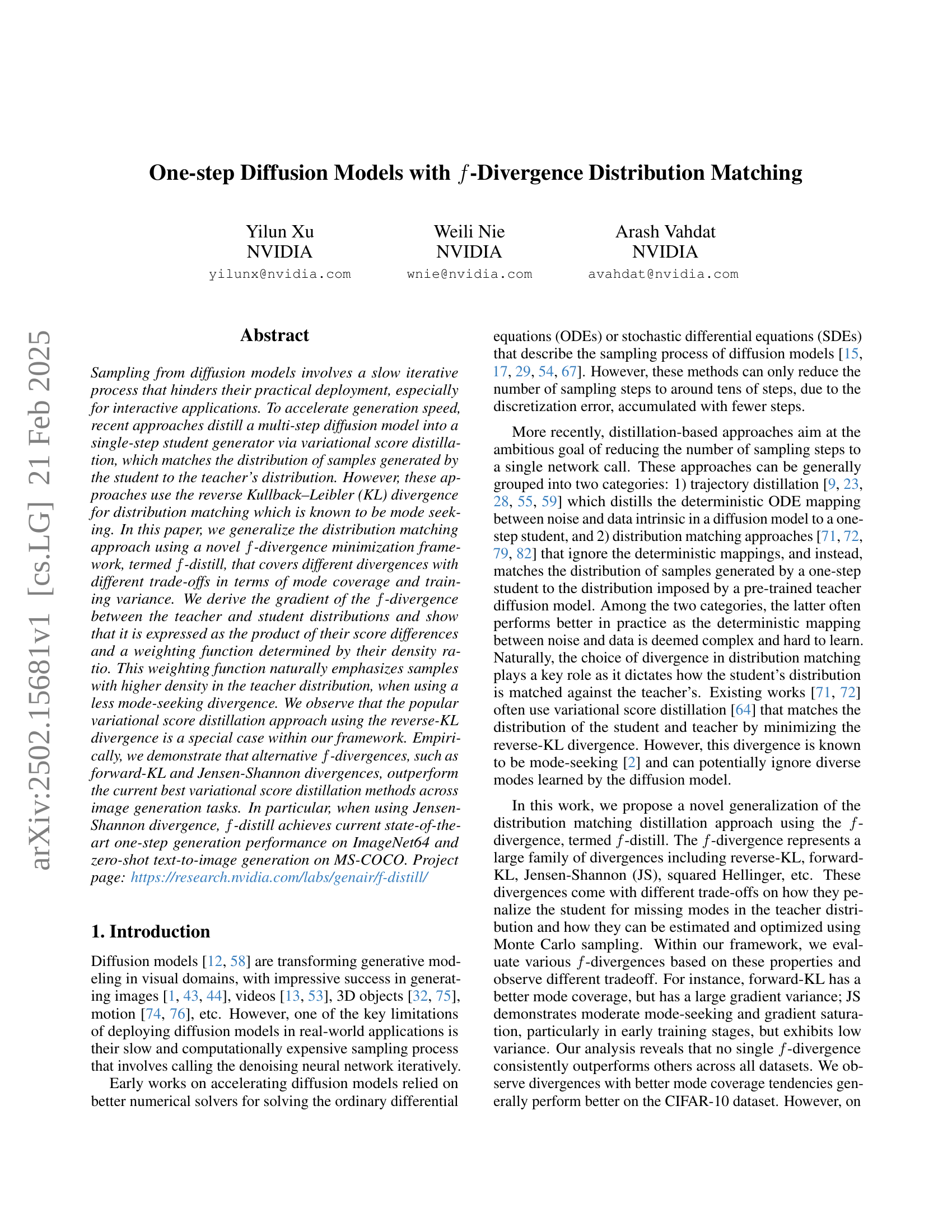
🔼 Figure 1 illustrates the training process for a one-step diffusion model using the proposed f-distill method. The core idea is to match the distribution of samples generated by a simplified, one-step student model to that of a more complex, multi-step teacher model. This is achieved by minimizing an f-divergence between the teacher and student sample distributions. The gradient update equation for the student model is shown. It reveals three key components: (1) the difference between the teacher’s score (gradient of the log-probability density) and the student’s (fake) score, (2) a weighting function determined by the f-divergence chosen and the density ratio between the teacher and student distributions, and (3) the gradient of the student’s generative function. The weighting function dynamically adjusts the contribution of samples from different density regions, ensuring stability and improved accuracy. Critically, the density ratio, which acts as a weight factor emphasizing high-density samples in the teacher distribution, is easily obtained from an auxiliary GAN (Generative Adversarial Network) objective. This GAN discriminator allows for direct calculation of the density ratio, streamlining the calculation and improving computational efficiency.
read the caption
Figure 1: The gradient update for the one-step student in f𝑓fitalic_f-distill. The gradient is a product of the difference between the teacher score and fake score, and a weighting function determined by the chosen f𝑓fitalic_f-divergence and density ratio. The density ratio is readily available from the discriminator in the auxiliary GAN objective.
| Mode-seeking? | Saturation? | Variance | |||
| reverse-KL | Yes | No | - | ||
| softened RKL | Yes | No | Low | ||
| Jensen-Shannon | Medium | Yes | Low | ||
| squared Hellinger | Medium | Yes | Low | ||
| forward-KL | No | No | High | ||
| Jeffreys | No | No | High |
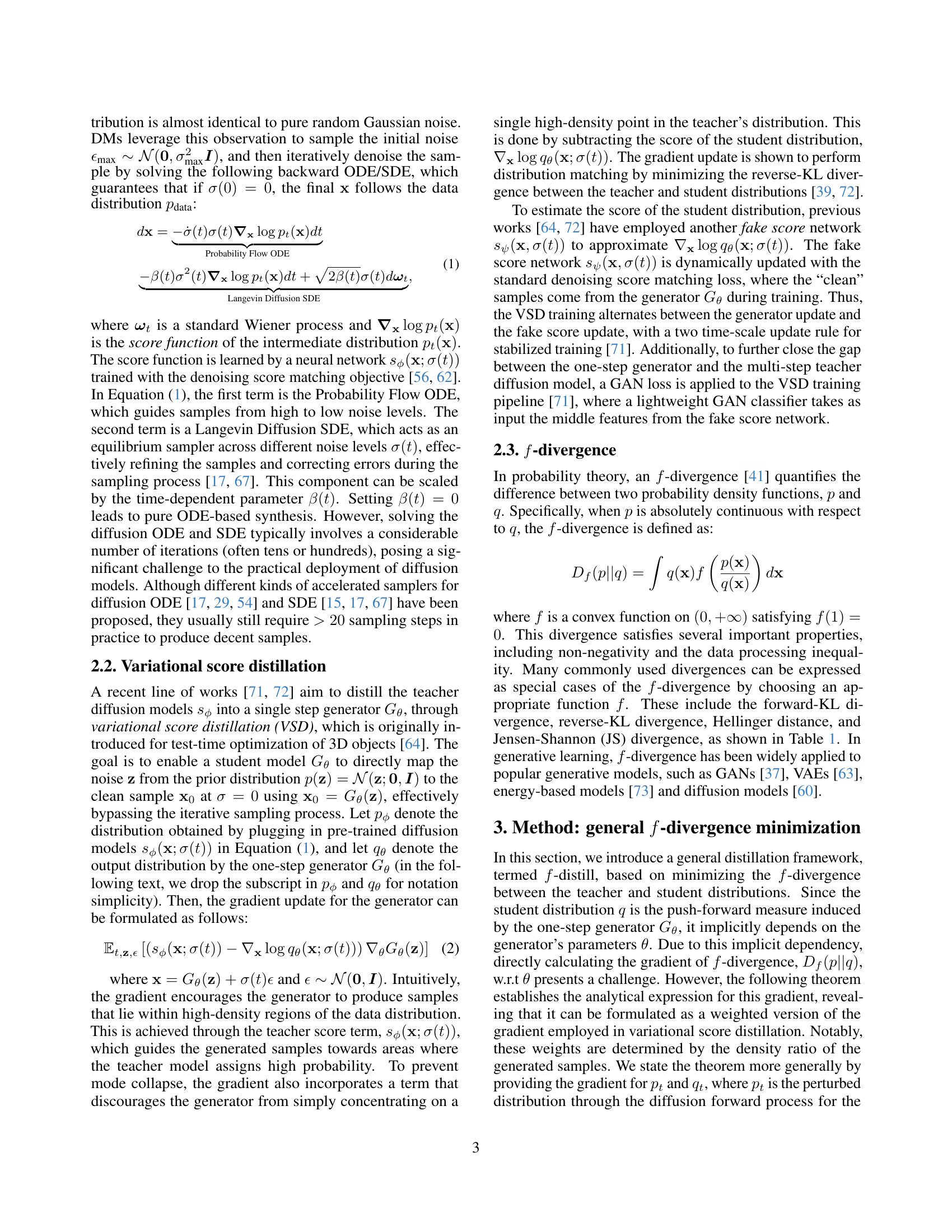
🔼 This table compares several f-divergences used in the paper’s proposed f-distill method. For each divergence, it lists the formula as a function of the likelihood ratio r (the ratio of the probability density functions of the teacher and student models), whether it tends to be mode-seeking (meaning it focuses on high-density regions and potentially ignores less prominent modes), whether the gradient tends to saturate during training, and the variance of the gradient. The table helps to understand the trade-offs between mode coverage, gradient stability, and training efficiency of different f-divergences.
read the caption
Table 1: Comparison of different f𝑓fitalic_f-divergences as a function of the likelihood ratio r:=p(𝐱)/q(𝐱)assign𝑟𝑝𝐱𝑞𝐱r:=p({\mathbf{x}})/q({\mathbf{x}})italic_r := italic_p ( bold_x ) / italic_q ( bold_x )
In-depth insights#
f-distill: Novel Distillation#
f-distill: Novel Distillation is a technique to distill knowledge from a larger, more complex model (teacher) into a smaller, faster one (student). The main idea is to train the student model to match the output distribution of the teacher model, using f-divergences as a measure of similarity. A key insight is that different f-divergences have different properties in terms of mode coverage and training stability. By carefully choosing the f-divergence, we can trade off these properties to achieve better performance on specific tasks. The core of f-distill lies in deriving a novel gradient update rule that elegantly combines the score differences of the teacher and student, weighted by a function of their density ratio. This weighting naturally emphasizes regions where the teacher is more confident, leading to more robust and efficient learning. This contrasts with previous methods like variational score distillation, which essentially use a fixed weighting (reverse-KL) and may suffer from mode-seeking behavior. f-distill provides a flexible framework for distribution matching distillation.
Mode-Seeking Tradeoffs#
Mode-seeking behavior in generative models, particularly concerning f-divergences, presents a crucial tradeoff. Mode-seeking divergences like reverse-KL encourage capturing only a subset of data modes, sacrificing diversity. While advantageous for some applications prioritizing specific, well-defined outputs, it’s detrimental in scenarios demanding comprehensive data representation. Less mode-seeking divergences, such as forward-KL, aim for mode coverage but face challenges like higher variance and potential instability during training. Balancing this tradeoff is essential. The choice of divergence significantly impacts the generated samples’ diversity and fidelity, demanding careful consideration of the application’s requirements. Techniques to mitigate the drawbacks of both approaches, like weighting functions, are vital for achieving optimal performance.
Divergence Variance#
The variance across different divergences in generative models is an essential consideration. High variance can lead to unstable training, where the model struggles to converge on an optimal solution. This instability often manifests as mode collapse or difficulty in generating diverse samples. The models utilize a normalized variance to measure the variance of different fs. For example, forward-KL divergence has a better mode coverage but it shows large gradient variance. By maintaining a balance between mode coverage and training variance, generative models are more likely to produce high-quality, diverse results consistently. Normalization techniques are often employed to mitigate high variance and stabilize training. Lower-variance divergences tend to perform better in generating realistic images since they are less prone to gradient explosion. The weight function’s variance in the ultimate purpose is critical for mini-batch training’s stability.
GAN Objective Impact#
The paper explores the impact of the GAN objective on diffusion distillation, highlighting its crucial role in enhancing performance. The GAN objective enables the student generator to surpass the teacher’s limitations, by leveraging real data through a discriminator. Ablation studies confirm the relative ranking of FID scores by different f-divergences remains consistent with or without GAN loss. This suggests that the GAN objective provides additional guidance, helping the student better approximate the data distribution. While variational score distillation relies on the teacher’s score function, the GAN objective acts as a supplementary force, leading to improved sample quality and stability. The auxiliary GAN objective as in prior work offers the additional advantage of providing a readily available estimate of the density ratio required by the weighting function, which facilitating the computation of the weighting function.
Inaccurate Ratios#
Inaccurate ratios within generative models, particularly diffusion models distilled for one-step generation, pose a significant challenge. The core issue stems from the discriminator’s difficulty in accurately estimating the density ratio between the generated (student) and real (teacher) distributions, especially in the early stages of training or in regions of low data density. This inaccuracy undermines the weighting function in f-divergence minimization, leading to suboptimal gradient updates. A poorly estimated ratio can either overemphasize noisy gradients from unreliable regions or suppress crucial updates needed to capture diverse modes. Techniques to mitigate this include carefully warming up the discriminator, employing robust normalization schemes, or leveraging more stable divergence formulations less sensitive to ratio errors. Addressing inaccurate ratios is paramount for achieving high-fidelity and diverse generations.
More visual insights#
More on figures

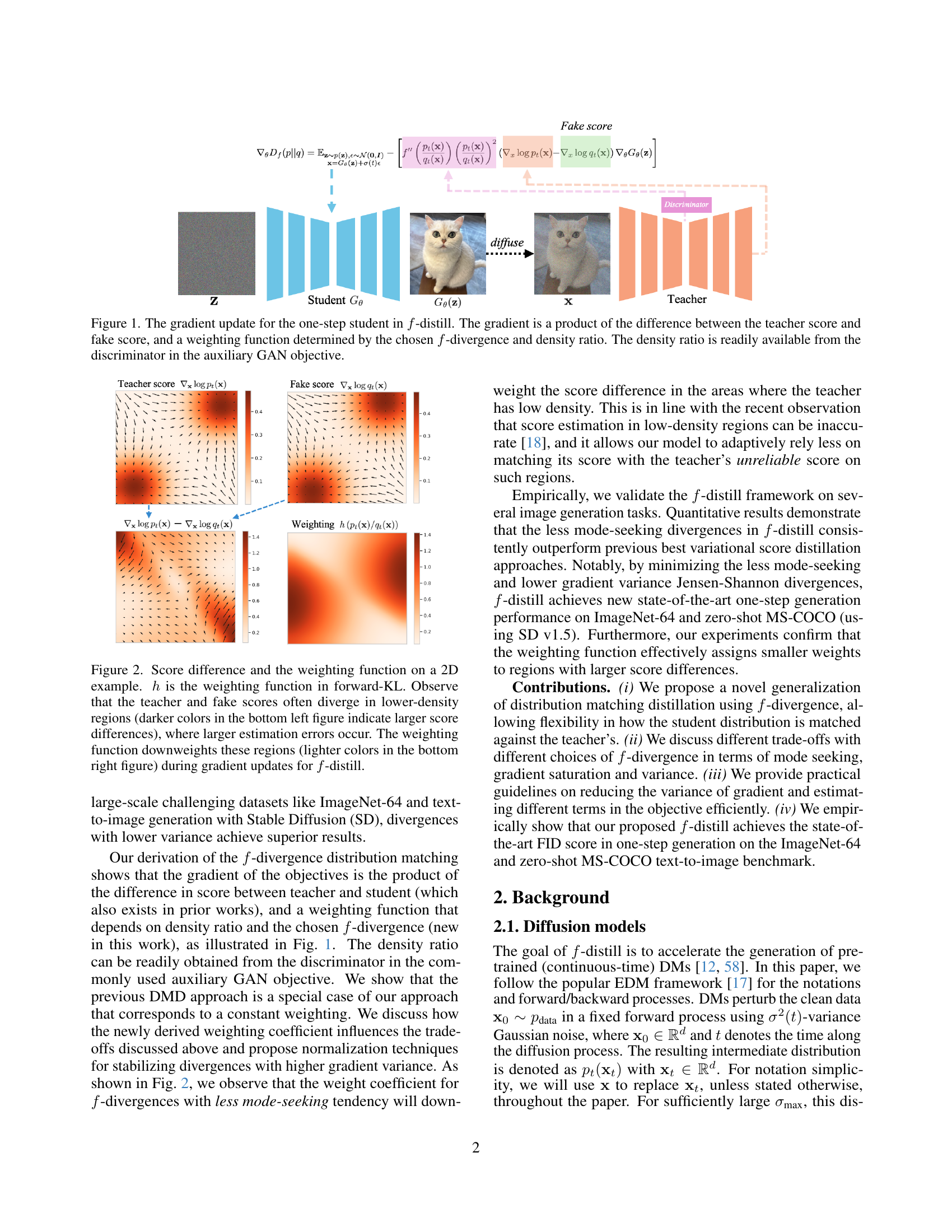
🔼 Figure 2 visualizes the concept of f-divergence distribution matching in a 2D setting. It displays the difference between the teacher and student scores (left) and the weighting function h (right) in forward-KL divergence. The visualization shows that significant score discrepancies occur in low-density regions of the teacher distribution (darker areas in the left panel). Crucially, the weighting function h down-weights these low-density areas (lighter areas in the right panel) during the gradient updates. This behavior, characteristic of f-distill, reduces the influence of potentially inaccurate score estimations in low-density regions, leading to more stable training and improved performance.
read the caption
Figure 2: Score difference and the weighting function on a 2D example. hℎhitalic_h is the weighting function in forward-KL. Observe that the teacher and fake scores often diverge in lower-density regions (darker colors in the bottom left figure indicate larger score differences), where larger estimation errors occur. The weighting function downweights these regions (lighter colors in the bottom right figure) during gradient updates for f𝑓fitalic_f-distill.

🔼 The figure shows the absolute value of the derivative of the f-divergence function (f’(r)) and the weighting function (h(r)) for different f-divergences. The x-axis represents the likelihood ratio (r = p(x)/q(x)), and the y-axis represents the value of f’(r) or h(r). Different lines correspond to different f-divergences, including reverse-KL, softened RKL, Jensen-Shannon, squared Hellinger, forward-KL, and Jeffreys. The figure demonstrates the different behaviors of these f-divergences in terms of their gradient and how their weighting function affects the gradient update in the f-distill framework.
read the caption
(a)

🔼 The figure shows the weighting function h(r) for different f-divergences as a function of the likelihood ratio r = p(x)/q(x). The weighting function h(r) is a key component in the proposed f-distill framework, which generalizes the distribution matching distillation approach using the f-divergence. The weighting function determines how the score differences between the teacher and student distributions are emphasized during gradient updates. The plot illustrates the trade-offs between different f-divergences in terms of mode-seeking behavior and variance. Less mode-seeking divergences have weighting functions that emphasize high-density regions in the teacher distribution more significantly, leading to better mode coverage but potentially higher variance.
read the caption
(b)

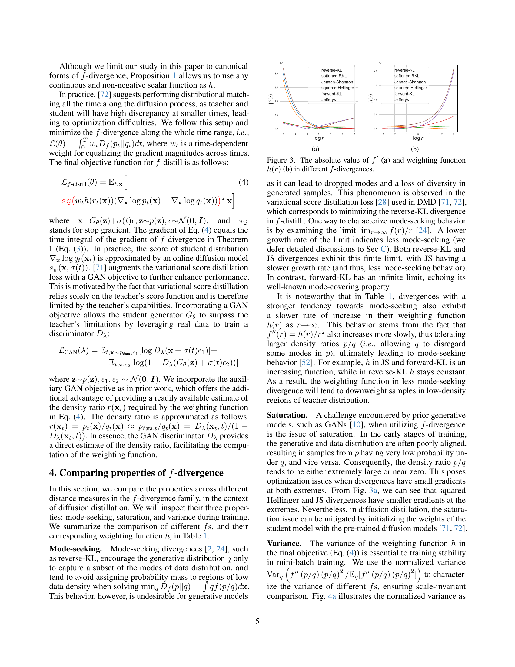
🔼 Figure 3 visualizes the properties of different f-divergences used in the f-distill framework. Panel (a) displays the absolute values of the first derivative of each f-divergence’s function (f′), showing how sensitive the f-divergence is to changes in the likelihood ratio. Panel (b) plots the weighting function, h(r), which is derived from the second derivative of the f-divergence and determines how much weight is given to score differences based on the density ratio (r=p(x)/q(x)) during training. By observing the differences in f′ and h(r) across these divergences, one can understand their different tradeoffs between mode-seeking tendency and training stability, which have important implications for the overall model performance.
read the caption
Figure 3: The absolute value of f′superscript𝑓′f^{\prime}italic_f start_POSTSUPERSCRIPT ′ end_POSTSUPERSCRIPT (a) and weighting function h(r)ℎ𝑟h(r)italic_h ( italic_r ) (b) in different f𝑓fitalic_f-divergences.

🔼 The figure shows the absolute values of the derivative of the f-divergence function (f’(r)) and the weighting function (h(r)) for different f-divergences. The x-axis represents the likelihood ratio (r), and the y-axis represents the values of f’(r) and h(r). The plots illustrate how different f-divergences, such as reverse-KL, Jensen-Shannon, and forward-KL, have varying gradients and weighting functions, impacting the mode-seeking properties and the training stability in the distribution matching distillation approach.
read the caption
(a)

🔼 The figure shows the absolute value of the derivative of the f-divergence (f’(r)) and the weighting function (h(r)) for different f-divergences as a function of the likelihood ratio (r). The derivative f’(r) shows how sensitive the f-divergence is to changes in the likelihood ratio, influencing the magnitude of gradient updates during training. The weighting function h(r), derived from the second derivative of the f-divergence, highlights how each divergence prioritizes samples from different regions of the teacher distribution. Specifically, it demonstrates how mode-seeking divergences, such as reverse KL, assign nearly uniform weights, while less mode-seeking divergences, like forward KL, emphasize high-density regions of the teacher distribution, making them less prone to ignoring under-represented data modes during training.
read the caption
(b)

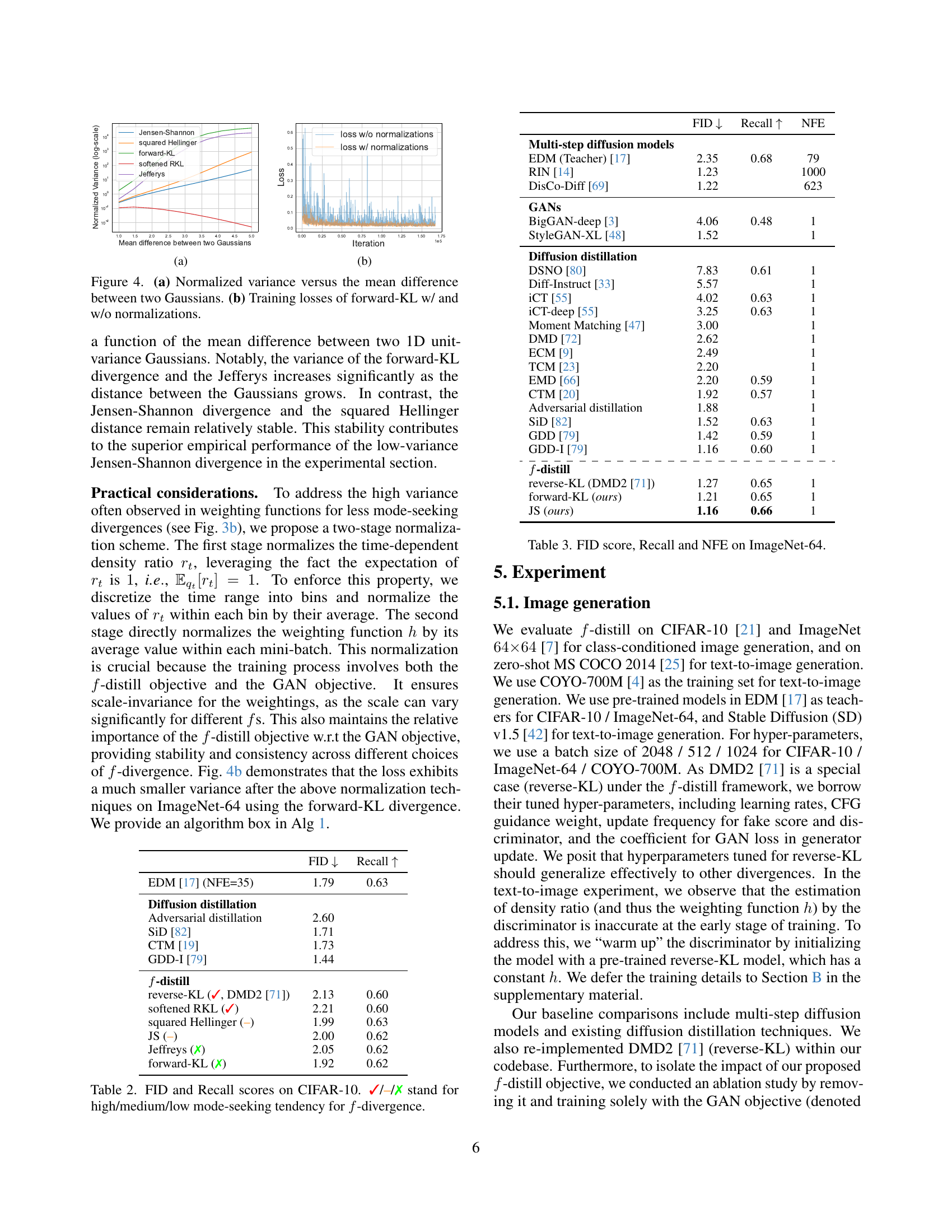
🔼 Figure 4(a) shows the relationship between the normalized variance of the weighting function and the mean difference between two 1D unit-variance Gaussian distributions. The normalized variance is calculated using the formula: Varq(f″(p/q)(p/q)²)/Eq[f″(p/q)(p/q)²]. This figure illustrates how the variance of the weighting function changes as the distance between the two Gaussian distributions increases. Figure 4(b) shows the training loss curves for the forward-KL divergence with and without the normalization techniques proposed in the paper. The figure demonstrates the effectiveness of the normalization techniques in reducing the variance of the gradients during training, which improves the stability of the training process.
read the caption
Figure 4: (a) Normalized variance versus the mean difference between two Gaussians. (b) Training losses of forward-KL w/ and w/o normalizations.

🔼 The figure shows the absolute value of the derivative of the f-divergence function (f’(r)) and the weighting function (h(r)) for different f-divergences. The x-axis represents the likelihood ratio (r = p(x)/q(x)), where p(x) is the teacher distribution and q(x) is the student distribution. The y-axis represents the values of f’(r) and h(r). Different lines represent different f-divergences (reverse-KL, softened RKL, Jensen-Shannon, squared Hellinger, forward-KL, Jefferys). The plot visually demonstrates how the weighting function h(r), derived from the second derivative of the f-divergence, varies across different divergences, which is crucial in determining the behavior of the gradient update in f-distill (f-divergence distribution matching). This variation highlights the different trade-offs in mode-seeking behavior and variance between various divergences used in the algorithm.
read the caption
(a)

🔼 The weighting function h(r) for different f-divergences plotted against the likelihood ratio r. The graph shows how the weight assigned to the score difference between the teacher and student models varies depending on the density ratio. The weighting function plays a key role in how f-distill balances mode coverage and training stability, with different f-divergences exhibiting different behaviors. The plot helps illustrate the trade-offs between mode-seeking and variance in different f-divergences.
read the caption
(b)

🔼 The figure shows a comparison of the weighting function, h(r), across different f-divergences. The weighting function is a crucial component in the f-distill framework, as it determines how much weight is assigned to different regions in the distribution based on the density ratio between the teacher and student. The figure visually demonstrates the different properties of each f-divergence, highlighting the impact on training stability and mode coverage. By understanding the behavior of the weighting function, one can better select an appropriate f-divergence for distribution matching in diffusion models.
read the caption
(c)

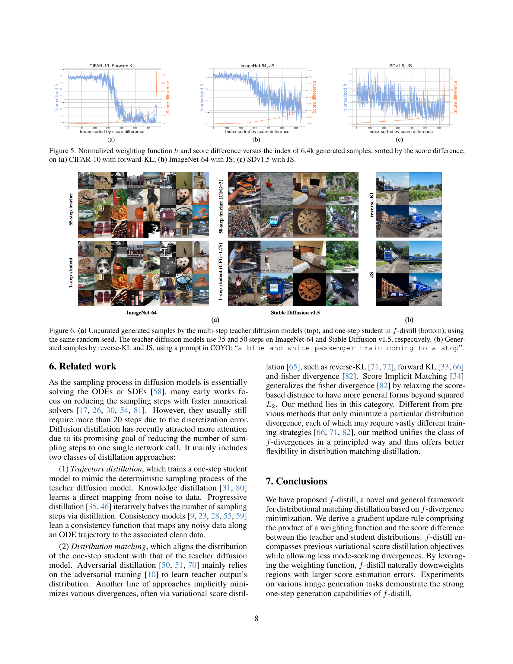
🔼 This figure visualizes the relationship between the normalized weighting function (h) and the score difference for 6,400 generated samples. The samples are sorted by their score difference. The score difference is calculated between the teacher’s score and the student’s (fake) score. Three subplots are shown, each representing a different dataset and f-divergence: (a) CIFAR-10 with forward-KL divergence; (b) ImageNet-64 with Jensen-Shannon (JS) divergence; and (c) Stable Diffusion v1.5 with JS divergence. The weighting function (h) is derived from the chosen f-divergence and is designed to emphasize samples with higher density in the teacher distribution when a less mode-seeking divergence is used, thus influencing the impact of score differences during training.
read the caption
Figure 5: Normalized weighting function hℎhitalic_h and score difference versus the index of 6.4k generated samples, sorted by the score difference, on (a) CIFAR-10 with forward-KL; (b) ImageNet-64 with JS; (c) SDv1.5 with JS.

🔼 Figure 6 demonstrates the image generation capabilities of the proposed f-distill method compared to a multi-step teacher model. Part (a) shows uncurated samples generated by the teacher model (using 35 steps for ImageNet64 and 50 steps for Stable Diffusion v1.5) and the one-step f-distill student model, both using the same random seed. This showcases the ability of f-distill to significantly reduce the number of sampling steps while maintaining comparable image quality. Part (b) presents a comparison of image generation using two different f-divergences within the f-distill framework (reverse-KL and Jensen-Shannon) for the same text prompt: “a blue and white passenger train coming to a stop”. This illustrates the impact of f-divergence choice on the resulting image generation.
read the caption
Figure 6: (a) Uncurated generated samples by the multi-step teacher diffusion models (top), and one-step student in f𝑓fitalic_f-distill (bottom), using the same random seed. The teacher diffusion models use 35 and 50 steps on ImageNet-64 and Stable Diffusion v1.5, respectively. (b) Generated samples by reverse-KL and JS, using a prompt in COYO: “a blue and white passenger train coming to a stop”.

🔼 The figure shows the absolute value of the derivative of the f-divergence function (f’(r)) and the weighting function (h(r)) for different f-divergences. The x-axis represents the likelihood ratio (r = p(x)/q(x)), where p(x) is the probability density of the teacher model and q(x) is the probability density of the student model. The y-axis represents the value of f’(r) or h(r). The plots illustrate the different properties of these functions and how they vary across different choices of f-divergence. Understanding these properties is important for selecting the most appropriate f-divergence for distribution matching in diffusion models. The weighting function emphasizes samples with higher densities in the teacher distribution when using a less mode-seeking divergence.
read the caption
(a)

🔼 The figure shows the weighting function h(r) for different f-divergences as a function of the likelihood ratio r. The weighting function is a key component of the f-distill framework, which uses f-divergences to match the distributions of the teacher and student models. The weighting function h(r) emphasizes samples with higher density in the teacher distribution, leading to better mode coverage. The plot shows that the weighting function h(r) varies significantly across different f-divergences, with some divergences showing a higher weight in high-density regions and others in low-density regions. This variation in the weighting function h(r) is crucial for achieving the state-of-the-art one-step generation performance in the f-distill framework.
read the caption
(b)

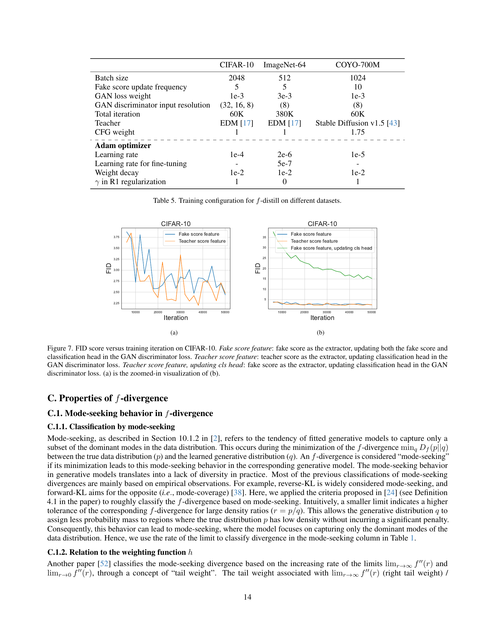
🔼 This figure compares the training performance of different variations of the f-distill method on the CIFAR-10 dataset. Three experimental setups are compared: using the fake score network’s output to update both the fake score and the classifier in the GAN discriminator (Fake score feature), using the teacher score network’s output to update only the classifier (Teacher score feature), and using the fake score network’s output but only updating the classifier (Teacher score feature, updating cls head). The plot shows FID score (lower is better) over training iterations. The second plot (b) shows the entire training run, while the first plot (a) is a zoomed-in view of the more interesting part of the training.
read the caption
Figure 7: FID score versus training iteration on CIFAR-10. Fake score feature: fake score as the extractor, updating both the fake score and classification head in the GAN discriminator loss. Teacher score feature: teacher score as the extractor, updating classification head in the GAN discriminator loss. Teacher score feature, updating cls head: fake score as the extractor, updating classification head in the GAN discriminator loss. (a) is the zoomed-in visualization of (b).

🔼 Figure 8 illustrates the effect of the weighting function ℎh in f-divergence on the learning process of generative models. The figure compares two scenarios: one using a less mode-seeking divergence (forward KL divergence) where the weighting function ℎh is proportional to the ratio of the teacher and student probability densities (ℎ=𝑝/𝑞h=p/q), and another using a more mode-seeking divergence (reverse KL divergence) where ℎ=1h=1. The plots show that with a less mode-seeking divergence and its corresponding weighting function, the model can better learn the true data distribution by capturing various modes, even when starting from a skewed initial generative distribution. This is achieved because the weighting function down-weights samples from low-density regions and thus prevents the model from overemphasizing high density regions, unlike the mode-seeking divergence.
read the caption
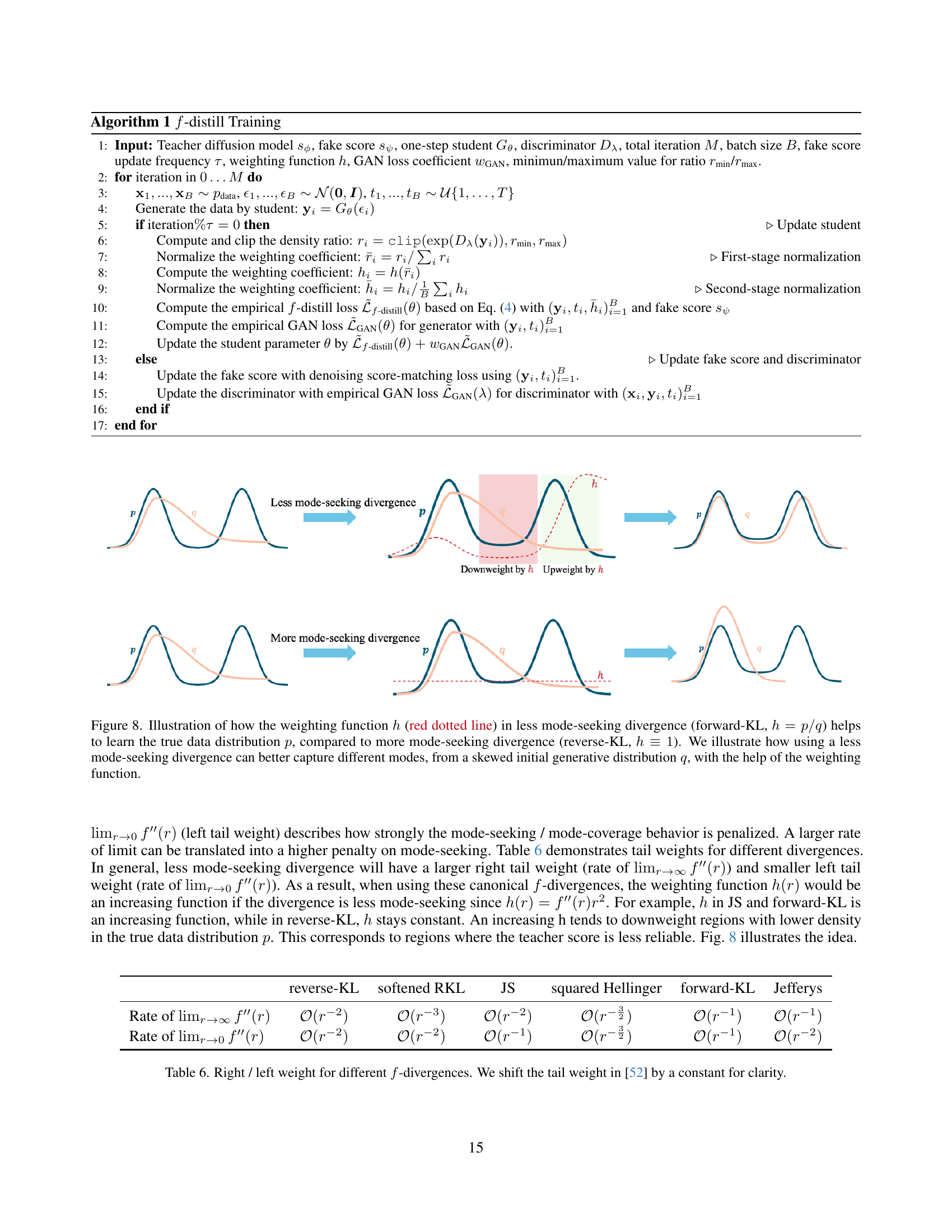
Figure 8: Illustration of how the weighting function hℎhitalic_h (red dotted line) in less mode-seeking divergence (forward-KL, h=p/qℎ𝑝𝑞h=p/qitalic_h = italic_p / italic_q) helps to learn the true data distribution p𝑝pitalic_p, compared to more mode-seeking divergence (reverse-KL, h≡1ℎ1h\equiv 1italic_h ≡ 1). We illustrate how using a less mode-seeking divergence can better capture different modes, from a skewed initial generative distribution q𝑞qitalic_q, with the help of the weighting function.

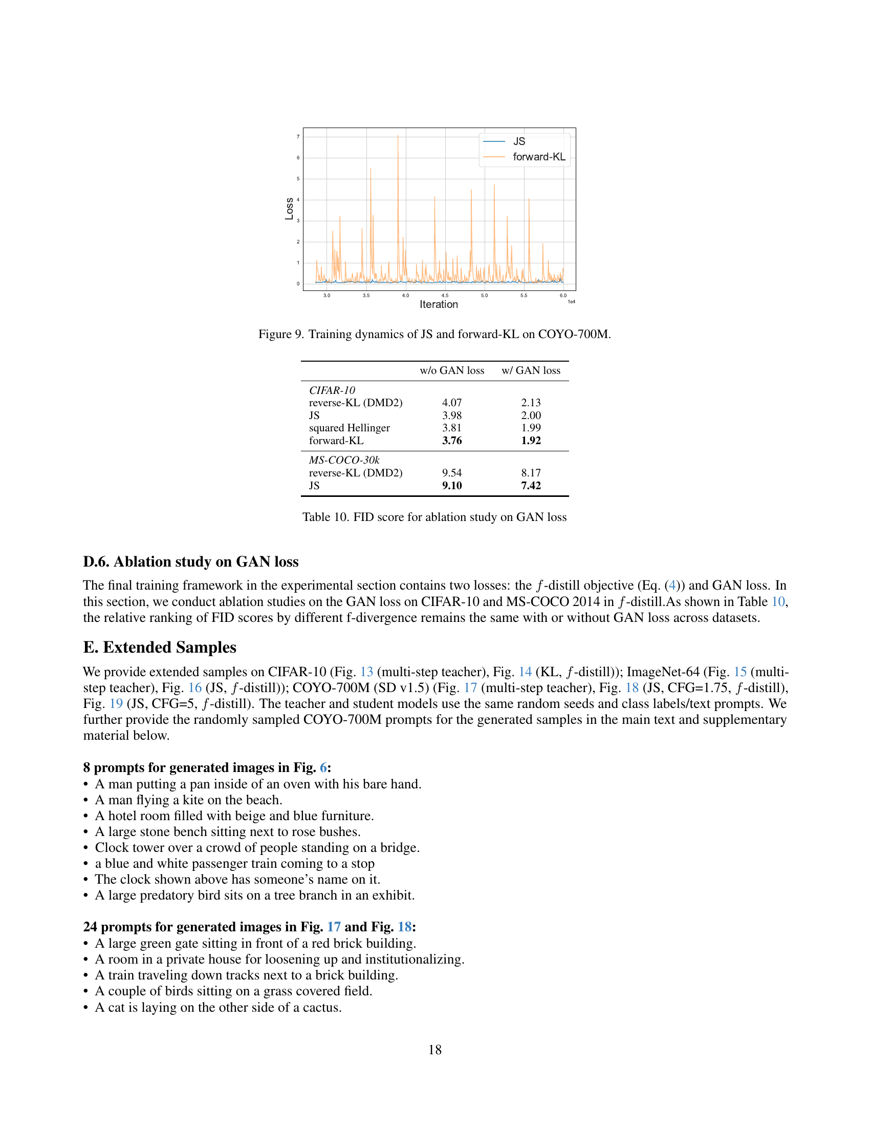
🔼 This figure compares the training loss curves for the Jensen-Shannon (JS) divergence and the forward Kullback-Leibler (forward-KL) divergence during the training process of the f-distill model on the COYO-700M dataset. The x-axis represents training iterations, and the y-axis represents the value of the loss function. The plot shows the training loss for JS divergence and the training loss for forward-KL divergence. By comparing the loss curves of these two methods, we can understand the effect of different choices of f-divergences on training stability, and whether one method provides better stability than the other during model training.
read the caption
Figure 9: Training dynamics of JS and forward-KL on COYO-700M.

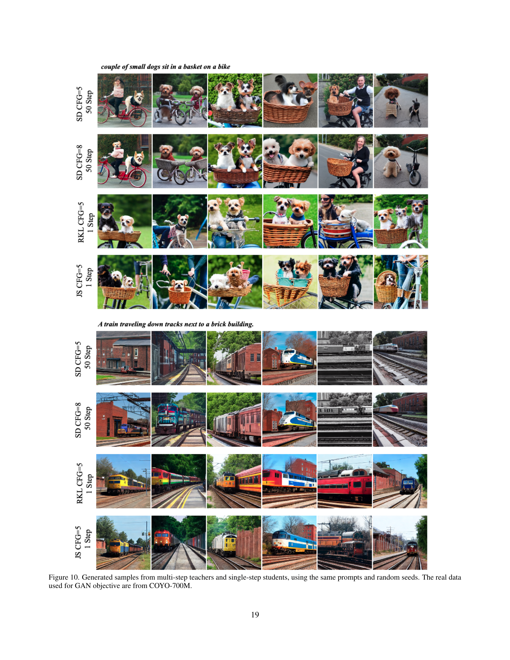
🔼 This figure compares image generation results from a multi-step teacher diffusion model and a single-step student model trained using the proposed f-distill method. The same prompts and random seeds were used for both models, ensuring a fair comparison. The images showcase the ability of the single-step student model to generate images comparable to the multi-step teacher model, highlighting the efficiency gains of f-distill. Real data from the COYO-700M dataset was used to train the GAN component in f-distill.
read the caption
Figure 10: Generated samples from multi-step teachers and single-step students, using the same prompts and random seeds. The real data used for GAN objective are from COYO-700M.

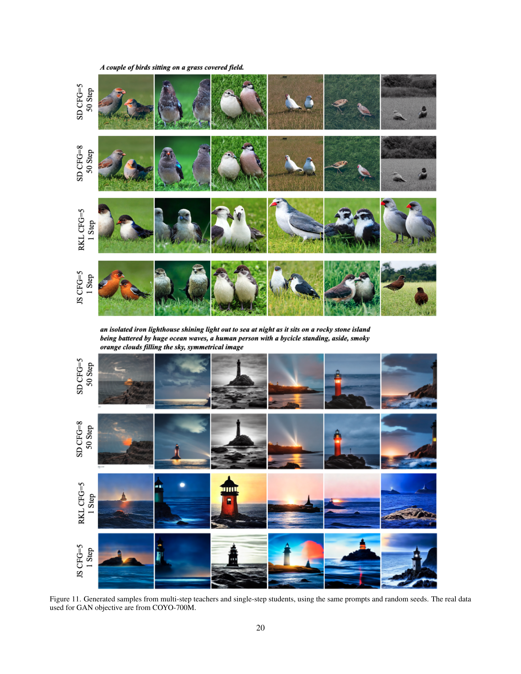
🔼 This figure compares image generation results from a multi-step diffusion model (teacher) and a single-step diffusion model (student) trained using the f-distill method. Both models were given the same prompts and random seeds, ensuring a fair comparison. The COYO-700M dataset was used as real data for the GAN (Generative Adversarial Network) objective in the f-distill training process. The images showcase the visual quality and diversity achievable by each model, illustrating the effectiveness of the f-distill method in distilling the knowledge of the complex multi-step diffusion model into a simplified one-step model.
read the caption
Figure 11: Generated samples from multi-step teachers and single-step students, using the same prompts and random seeds. The real data used for GAN objective are from COYO-700M.

🔼 This figure visualizes the results of image generation using both multi-step teacher diffusion models and single-step student models trained with the proposed f-distill method. The same prompts and random seeds are used for both types of models to ensure a fair comparison. The images show the generation quality from both models side-by-side for two different scenarios: a border collie surfing and a macro shot of a ladybug. The COYO-700M dataset is used as real data for training the GAN objective in the f-distill model.
read the caption
Figure 12: Generated samples from multi-step teachers and single-step students, using the same prompts and random seeds. The real data used for GAN objective are from COYO-700M.

🔼 This figure displays 35 images generated from a 35-step diffusion model (EDM [17]) trained on the CIFAR-10 dataset. These images represent a sample of the model’s output, showcasing its ability to generate diverse and realistic images of objects from the CIFAR-10 classes. The Fréchet Inception Distance (FID) score, a metric used to evaluate the quality of generated images by comparing them to real images, is reported as 1.79, indicating high image quality. A lower FID score indicates better performance.
read the caption
Figure 13: 35-step generated CIFAR-10 samples, by EDM [17] (teacher). FID score: 1.79

🔼 This figure displays images generated by a one-step diffusion model, specifically using the KL divergence method within the f-distill framework. The model generated these CIFAR-10 images in a single step, demonstrating the efficiency of this approach. The FID (Fréchet Inception Distance) score of 1.92 indicates the quality of the generated images relative to real CIFAR-10 images; a lower FID score suggests higher image quality and similarity to real data.
read the caption
Figure 14: One-step generated CIFAR-10 samples, by KL in f𝑓fitalic_f-distill. FID score: 1.92

🔼 This figure displays 79 samples generated from the ImageNet-64 dataset using the EDM (Energy-based Diffusion Model) method, which serves as the teacher model in this study. Each image is 64x64 pixels. The FID (Fréchet Inception Distance) score, a metric for evaluating the quality of generated images by comparing them to real images, is 2.35. A lower FID score indicates that the generated images are more realistic and similar to real images from the dataset.
read the caption
Figure 15: 79-step generated ImageNet-64 samples, by EDM [17] (teacher). FID score: 2.35

🔼 This figure displays images generated by a one-step diffusion model using the Jensen-Shannon (JS) divergence in the f-distill framework. The images are of size 64x64 and belong to the ImageNet-64 dataset. The FID score, a metric assessing the quality of generated images by comparing them to real images, is 1.16, indicating high-quality generation.
read the caption
Figure 16: One-step generated ImageNet-64 samples, by JS in f𝑓fitalic_f-distill. FID score: 1.16

🔼 This figure displays 16 images generated by a 50-step Stable Diffusion v1.5 model using prompts from the COYO-700M dataset. The model was run with a classifier-free guidance (CFG) scale of 3. The Fréchet Inception Distance (FID) score, a metric evaluating the quality of generated images, was 8.59. The images showcase the model’s ability to generate diverse and realistic images based on text prompts.
read the caption
Figure 17: 50-step generated SD v1.5 samples, using randomly sampled COYO-700M prompts, by SD v1.5 model [43] (teacher). CFG=3. FID score: 8.59

🔼 This figure displays images generated using a single-step method (f-distill with JS divergence) on the Stable Diffusion v1.5 model. The prompts used were randomly selected from the COYO-700M dataset. The FID (Fréchet Inception Distance) score, a common metric for evaluating the quality of generated images, is 7.42, indicating the quality of these generated images.
read the caption
Figure 18: One-step generated SD v1.5 samples, using randomly sampled COYO-700M prompts, by JS in f𝑓fitalic_f-distill, with CFG=1.75. FID score: 7.42
More on tables
| FID | Recall | |
| EDM [17] (NFE=35) | 1.79 | 0.63 |
| Diffusion distillation | ||
| Adversarial distillation | 2.60 | |
| SiD [82] | 1.71 | |
| CTM [19] | 1.73 | |
| GDD-I [79] | 1.44 | |
| -distill | ||
| reverse-KL (✓, DMD2 [71]) | 2.13 | 0.60 |
| softened RKL (✓) | 2.21 | 0.60 |
| squared Hellinger (–) | 1.99 | 0.63 |
| JS (–) | 2.00 | 0.62 |
| Jeffreys (✗) | 2.05 | 0.62 |
| forward-KL (✗) | 1.92 | 0.62 |
🔼 Table 2 presents a comparison of FID (Fréchet Inception Distance) and Recall scores achieved by different methods on the CIFAR-10 dataset for image generation. The methods compared include various f-divergence-based diffusion distillation techniques (as introduced in the paper), along with several existing adversarial and diffusion distillation methods. The FID score measures the quality of the generated images, while the Recall score indicates the diversity of those images. The table also notes the mode-seeking tendency of each f-divergence, categorized as high (✓), medium (–), or low (✗), which provides insights into how the different f-divergences balance mode coverage and the risk of model collapse. The results highlight the relative performance of different approaches for efficient image generation.
read the caption
Table 2: FID and Recall scores on CIFAR-10. ✓/–/✗ stand for high/medium/low mode-seeking tendency for f𝑓fitalic_f-divergence.
| FID | Recall | NFE | |
| Multi-step diffusion models | |||
| EDM (Teacher) [17] | 2.35 | 0.68 | 79 |
| RIN [14] | 1.23 | 1000 | |
| DisCo-Diff [69] | 1.22 | 623 | |
| GANs | |||
| BigGAN-deep [3] | 4.06 | 0.48 | 1 |
| StyleGAN-XL [48] | 1.52 | 1 | |
| Diffusion distillation | |||
| DSNO [80] | 7.83 | 0.61 | 1 |
| Diff-Instruct [33] | 5.57 | 1 | |
| iCT [55] | 4.02 | 0.63 | 1 |
| iCT-deep [55] | 3.25 | 0.63 | 1 |
| Moment Matching [47] | 3.00 | 1 | |
| DMD [72] | 2.62 | 1 | |
| ECM [9] | 2.49 | 1 | |
| TCM [23] | 2.20 | 1 | |
| EMD [66] | 2.20 | 0.59 | 1 |
| CTM [20] | 1.92 | 0.57 | 1 |
| Adversarial distillation | 1.88 | 1 | |
| SiD [82] | 1.52 | 0.63 | 1 |
| GDD [79] | 1.42 | 0.59 | 1 |
| GDD-I [79] | 1.16 | 0.60 | 1 |
| \cdashline1-4 | |||
| -distill | |||
| reverse-KL (DMD2 [71]) | 1.27 | 0.65 | 1 |
| forward-KL (ours) | 1.21 | 0.65 | 1 |
| JS (ours) | 1.16 | 0.66 | 1 |
🔼 This table presents a comparison of different generative models on the ImageNet-64 dataset, focusing on the Fréchet Inception Distance (FID) score, Recall, and Number of Forward Euler steps (NFE). Lower FID scores indicate better image quality, higher Recall scores represent greater diversity in the generated images, and lower NFE values demonstrate faster generation times. The table includes results from various multi-step diffusion models, adversarial distillation approaches, and the proposed f-distill method with different f-divergences.
read the caption
Table 3: FID score, Recall and NFE on ImageNet-64.
| FID | CLIP score | Latency | |
| Multi-step diffusion models | |||
| LDM [42] | 12.63 | 3.7s | |
| DALL·E 2 [40] | 10.39 | 27s | |
| Imagen [45] | 7.27 | 0.28* | 9.1s |
| eDiff-I [1] | 6.95 | 0.29* | 32.0s |
| UniPC [78] | 19.57 | 0.26s | |
| Restart [67] | 13.16 | 0.299 | 3.40s |
| \cdashline1-4 | |||
| Teacher | |||
| SDv1.5 (NFE=50, CFG=3, ODE) | 8.59 | 0.308 | 2.59s |
| SDv1.5 (NFE=200, CFG=2, SDE) | 7.21 | 0.301 | 10.25s |
| GANs | |||
| StyleGAN-T [49] | 13.90 | 0.29* | 0.10s |
| GigaGAN [16] | 9.09 | 0.13s | |
| Diffusion distillation | |||
| SwiftBrush [36] | 16.67 | 0.29* | 0.09s |
| SwiftBrush v2 [6] | 8.14 | 0.32* | 0.06s |
| HiPA [77] | 13.91 | 0.09s | |
| InstaFlow-0.9B [27] | 13.10 | 0.09s | |
| UFOGen [70] | 12.78 | 0.09s | |
| DMD [72] | 11.49 | 0.09s | |
| EMD [66] | 9.66 | 0.09s | |
| \cdashline1-4 | |||
| CFG=1.75 | |||
| reverse-KL (DMD2 [71]) | 8.17 | 0.287 | 0.09s |
| JS (ours) | 7.42 | 0.292 | 0.09s |
| \cdashline1-4 | |||
| CFG=5 | |||
| reverse-KL (DMD2 [71]) | 15.23 | 0.309 | 0.09s |
| JS (ours) | 14.25 | 0.311 | 0.09s |
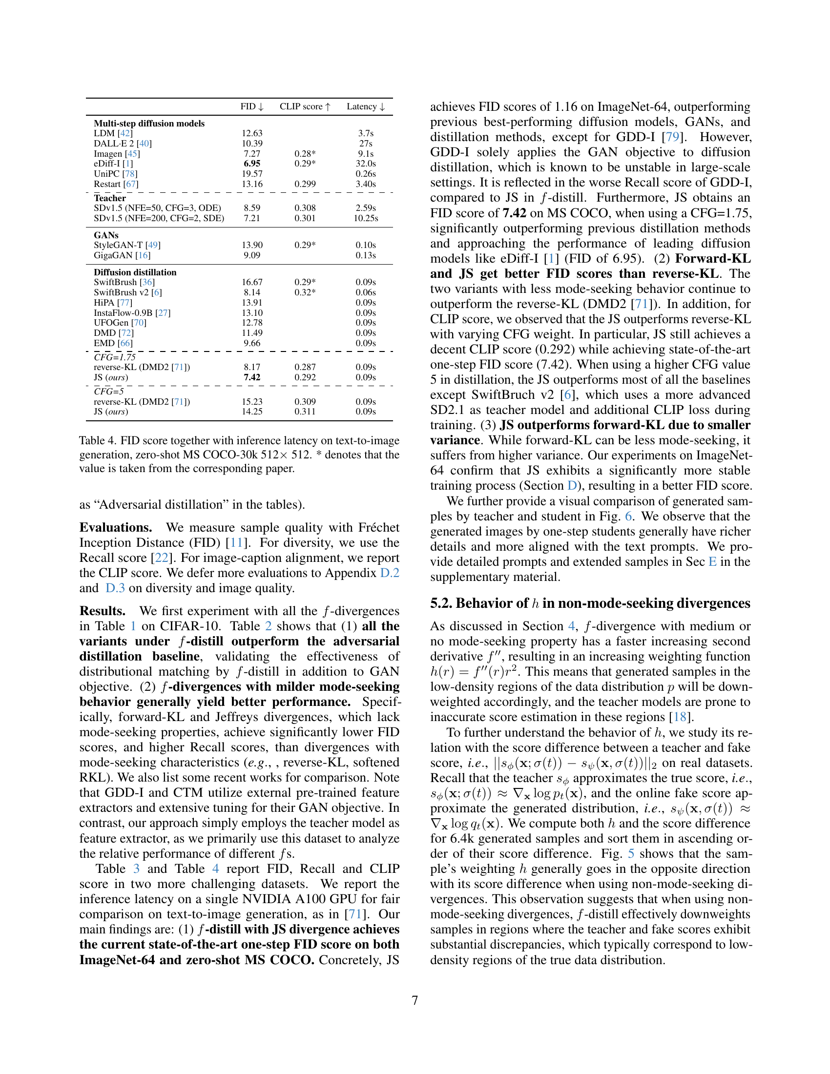
🔼 Table 4 presents a comparison of various text-to-image generation models, focusing on their performance on the MS COCO-30k dataset with images of size 512x512. The models are evaluated using the Fréchet Inception Distance (FID) score, a lower FID indicating better image quality, and inference latency (time to generate an image). The table includes both multi-step diffusion models and single-step approaches using diffusion distillation. It shows the FID score, recall, and number of forward diffusion steps (NFE) for each model. Results marked with an asterisk (*) indicate values obtained from published papers, as opposed to results from the current study.
read the caption
Table 4: FID score together with inference latency on text-to-image generation, zero-shot MS COCO-30k 512×\times× 512. * denotes that the value is taken from the corresponding paper.
| CIFAR-10 | ImageNet-64 | COYO-700M | |
| Batch size | 2048 | 512 | 1024 |
| Fake score update frequency | 5 | 5 | 10 |
| GAN loss weight | 1e-3 | 3e-3 | 1e-3 |
| GAN discriminator input resolution | (32, 16, 8) | (8) | (8) |
| Total iteration | 60K | 380K | 60K |
| Teacher | EDM [17] | EDM [17] | Stable Diffusion v1.5 [43] |
| CFG weight | 1 | 1 | 1.75 |
| \cdashline1-4 | |||
| Adam optimizer | |||
| Learning rate | 1e-4 | 2e-6 | 1e-5 |
| Learning rate for fine-tuning | - | 5e-7 | - |
| Weight decay | 1e-2 | 1e-2 | 1e-2 |
| in R1 regularization | 1 | 0 | 1 |
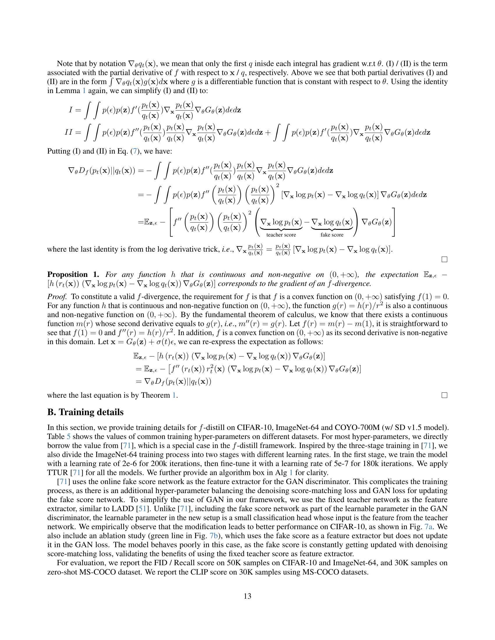
🔼 This table details the hyperparameters used in training the f-distill model on three different datasets: CIFAR-10, ImageNet-64, and COYO-700M. It shows settings for batch size, fake score update frequency, the weight assigned to the GAN loss, the resolution of the GAN discriminator’s input, and the total number of training iterations. It also lists hyperparameters specific to the Adam optimizer, including the learning rate, weight decay, and whether R1 regularization was used. Finally, it specifies the teacher model and corresponding configuration settings (CFG) used for each dataset.
read the caption
Table 5: Training configuration for f𝑓fitalic_f-distill on different datasets.
| reverse-KL | softened RKL | JS | squared Hellinger | forward-KL | Jefferys | |
| Rate of | ||||||
| Rate of |
🔼 This table compares different f-divergences based on their mode-seeking behavior, which is assessed by analyzing the rate of increase of their second derivative (f’’) at both extremes (0 and infinity). The ‘right tail weight’ represents how strongly the mode-seeking tendency is penalized as the likelihood ratio (p/q) becomes large, and the ’left tail weight’ reflects the behavior when the ratio is near zero. This analysis helps to understand how different f-divergences prioritize different modes (regions) within the data distribution. The tail weights are derived from previous work [52] but adjusted for consistency.
read the caption
Table 6: Right / left weight for different f𝑓fitalic_f-divergences. We shift the tail weight in [52] by a constant for clarity.
| FID | Recall | NFE | |
| Multi-step diffusion models | |||
| DDPM [12] | 3.17 | 1000 | |
| LSGM [61] | 2.10 | 138 | |
| EDM [17] (teacher) | 1.79 | 35 | |
| PFGM++ [68] | 1.74 | 35 | |
| GANs | |||
| BigGAN [3] | 14.73 | 1 | |
| StyleSAN-XL [48] | 1.36 | 1 | |
| Diffusion distillation | |||
| Adversarial distillation | 2.60 | 1 | |
| SiD () [82] | 1.93 | 1 | |
| SiD () [82] | 1.71 | 1 | |
| CTM [19] | 1.73 | 1 | |
| GDD [79] | 1.66 | 1 | |
| GDD-I [79] | 1.44 | 1 | |
| -distill | |||
| reverse-KL (✓, DMD2 [71]) | 2.13 | 0.60 | 1 |
| softened RKL (✓) | 2.21 | 0.60 | 1 |
| squared Hellinger (–) | 1.99 | 0.63 | 1 |
| JS (–) | 2.00 | 0.62 | 1 |
| Jeffreys (✗) | 2.05 | 0.62 | 1 |
| forward-KL (✗) | 1.92 | 0.62 | 1 |
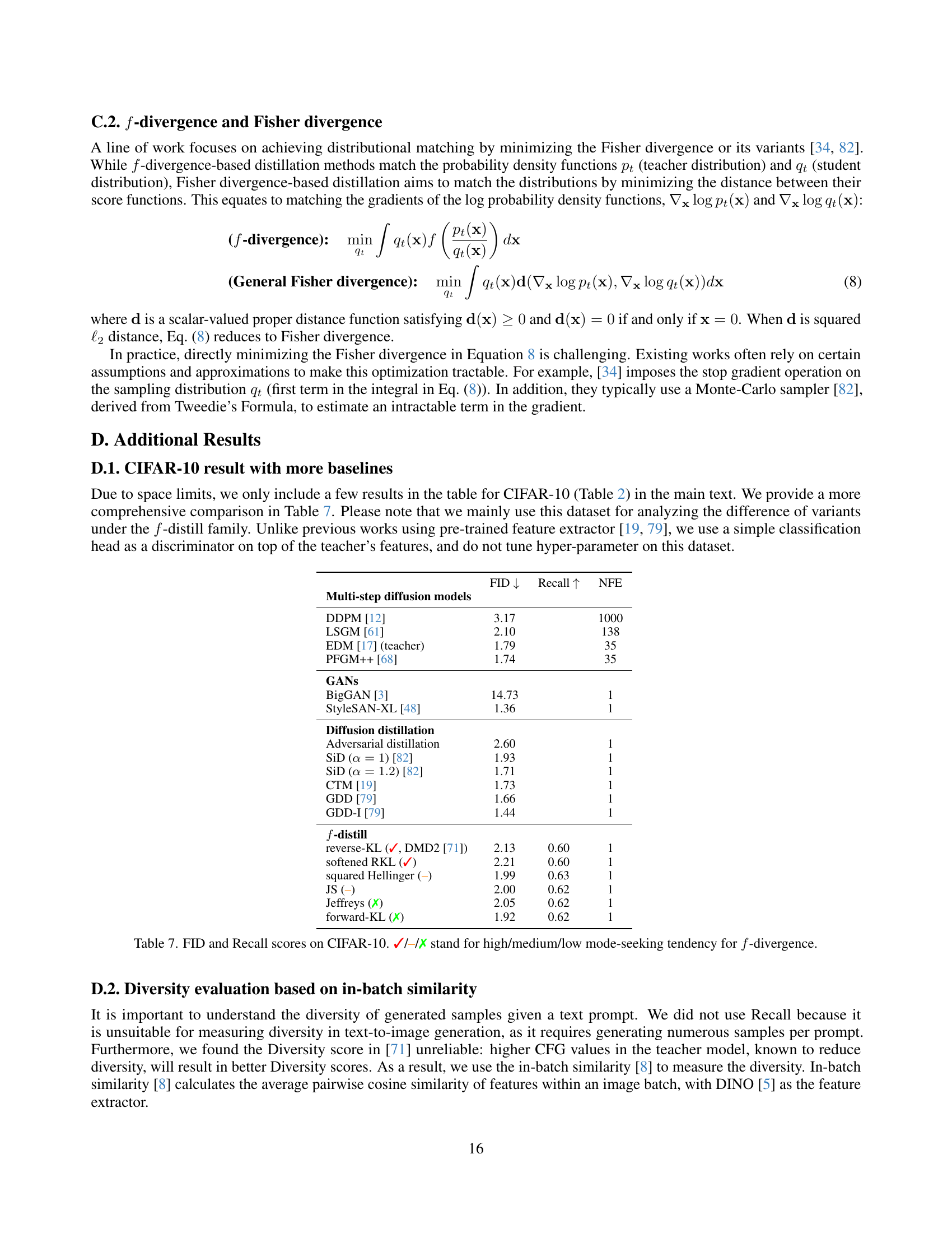
🔼 Table 7 presents a comparison of FID (Fréchet Inception Distance) and Recall scores achieved on the CIFAR-10 image generation task. It contrasts multiple methods: various f-divergence-based distillation approaches using the f-distill framework (reverse-KL, softened RKL, squared Hellinger, JS, Jefferys, and forward-KL), an adversarial distillation baseline, and several multi-step diffusion models. The ‘mode-seeking tendency’ column categorizes each f-divergence into high (✓), medium (–), or low (✗) based on how much the method focuses on matching only the most prominent modes of the data distribution, versus capturing the diversity of all modes. Lower FID scores indicate better image quality, while higher Recall scores show greater sample diversity.
read the caption
Table 7: FID and Recall scores on CIFAR-10. ✓/–/✗ stand for high/medium/low mode-seeking tendency for f𝑓fitalic_f-divergence.
| In-batch-sim | |
| SDv1.5 (NFE=50, CFG=3, ODE) | 0.55 / 0.70 |
| SDv1.5 (NFE=50, CFG=8, ODE) | 0.62 / 0.72 |
| \cdashline1-2 | |
| CFG=1.75 | |
| reverse-KL (DMD2 [71]) | 0.50 / 0.42 |
| JS (ours) | 0.49 / 0.41 |
| \cdashline1-2 | |
| CFG=5 | |
| reverse-KL (DMD2 [71]) | 0.67 / 0.60 |
| JS (ours) | 0.65 / 0.58 |
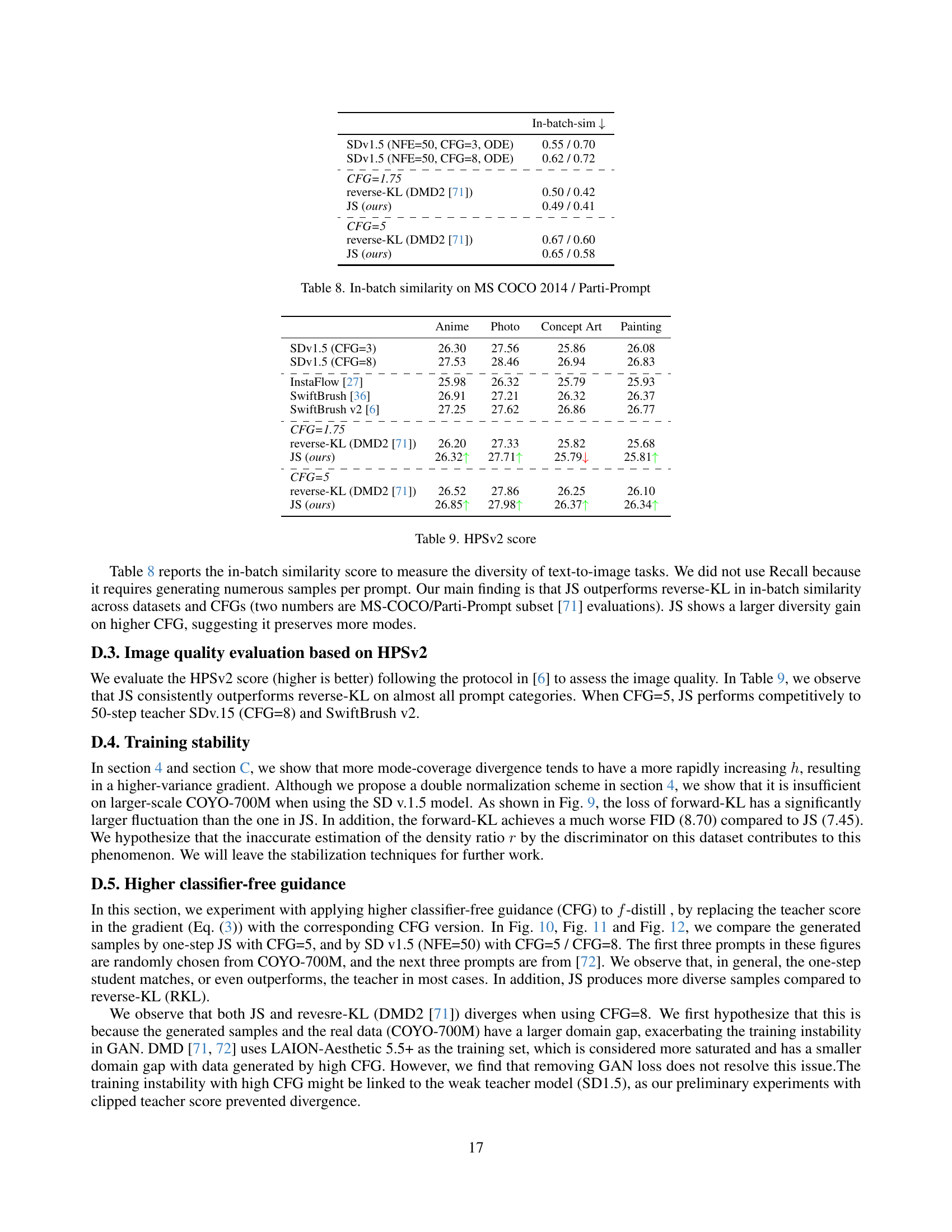
🔼 This table presents the in-batch similarity scores for generated images on the MS COCO 2014 dataset and its Parti-Prompt subset. In-batch similarity measures the average pairwise cosine similarity of image features within a batch, indicating image diversity. Lower scores suggest higher diversity. The table compares different methods and configurations, including varying classifier-free guidance (CFG) weights, to show how different approaches affect the diversity of generated images.
read the caption
Table 8: In-batch similarity on MS COCO 2014 / Parti-Prompt
| Anime | Photo | Concept Art | Painting | |
| SDv1.5 (CFG=3) | 26.30 | 27.56 | 25.86 | 26.08 |
| SDv1.5 (CFG=8) | 27.53 | 28.46 | 26.94 | 26.83 |
| \cdashline1-5 | ||||
| InstaFlow [27] | 25.98 | 26.32 | 25.79 | 25.93 |
| SwiftBrush [36] | 26.91 | 27.21 | 26.32 | 26.37 |
| SwiftBrush v2 [6] | 27.25 | 27.62 | 26.86 | 26.77 |
| \cdashline1-5 | ||||
| CFG=1.75 | ||||
| reverse-KL (DMD2 [71]) | 26.20 | 27.33 | 25.82 | 25.68 |
| JS (ours) | 26.32 | 27.71 | 25.79 | 25.81 |
| \cdashline1-5 | ||||
| CFG=5 | ||||
| reverse-KL (DMD2 [71]) | 26.52 | 27.86 | 26.25 | 26.10 |
| JS (ours) | 26.85 | 27.98 | 26.37 | 26.34 |
🔼 This table presents the HPSv2 scores, a metric for evaluating the quality of generated images. It compares the performance of different methods across four image categories: Anime, Photo, Concept Art, and Painting. The methods compared include the multi-step diffusion model (Stable Diffusion v1.5) with different CFG (classifier-free guidance) settings, as well as several one-step diffusion distillation methods, namely, reverse-KL (DMD2) and JS (from the proposed f-distill method), both with different CFG values. The scores show the relative quality of image generation for each method within each image category.
read the caption
Table 9: HPSv2 score
| w/o GAN loss | w/ GAN loss | |
| CIFAR-10 | ||
| reverse-KL (DMD2) | 4.07 | 2.13 |
| JS | 3.98 | 2.00 |
| squared Hellinger | 3.81 | 1.99 |
| forward-KL | 3.76 | 1.92 |
| MS-COCO-30k | ||
| reverse-KL (DMD2) | 9.54 | 8.17 |
| JS | 9.10 | 7.42 |
🔼 This table presents the Fréchet Inception Distance (FID) scores achieved by the proposed f-distill model with different f-divergences on two image generation datasets (CIFAR-10 and MS-COCO), both with and without the GAN loss component in the training objective. It demonstrates the impact of the GAN loss on model performance and helps assess the effectiveness of the f-divergence choices in the proposed model.
read the caption
Table 10: FID score for ablation study on GAN loss
Full paper#