DICEPTION: A Generalist Diffusion Model for Visual Perceptual Tasks

2502.17157

Canyu Zhao et el.

🤗 2025-02-25

TL;DR
#

Foundation models often need massive datasets and resources. In computer vision, task representations differ greatly, making it hard to create versatile solutions. Fine-tuning models for new tasks remains a challenge. Existing efforts fall short of specialized models, requiring costly training and data.

DICEPTION, is a diffusion model for many vision tasks, tackling challenges with limited resources. It matches state-of-the-art performance using a fraction of the data. By using color encoding for outputs, it allows use of pre-trained text-to-image models.DICEPTION trains efficiently and adapts to new tasks with minimal fine-tuning.

Key Takeaways
#

Why does it matter?
#

This paper introduces DICEPTION, a promising generalist visual model, pushing the boundaries of what’s achievable with limited data. It paves the way for more efficient and accessible AI solutions in various computer vision applications and open to future research.

Visual Insights
#

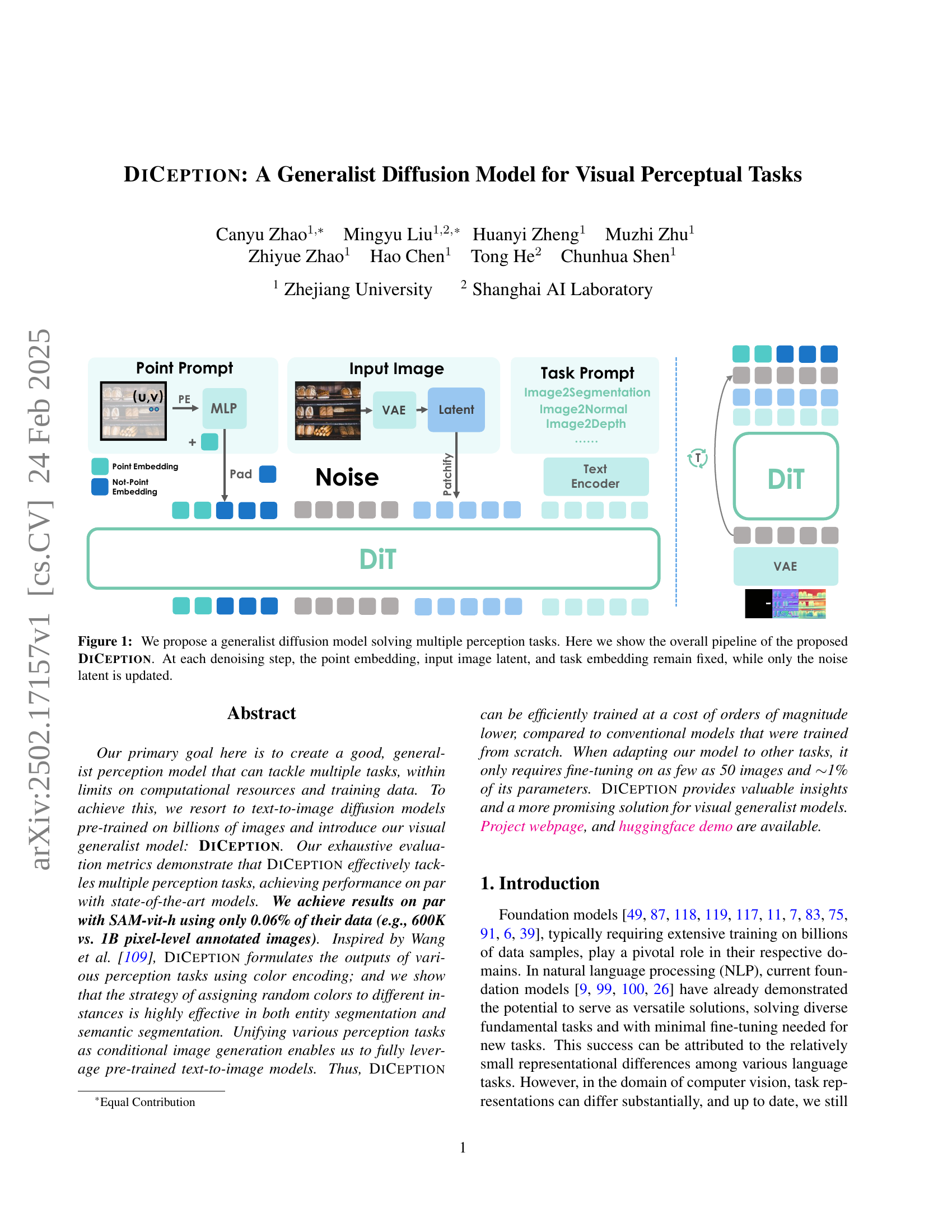
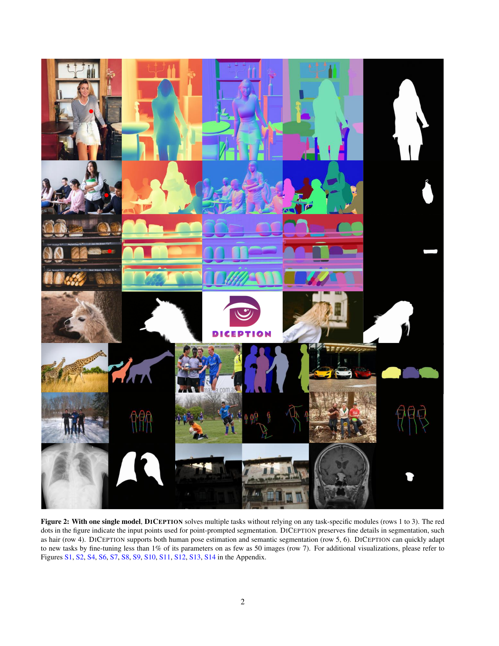
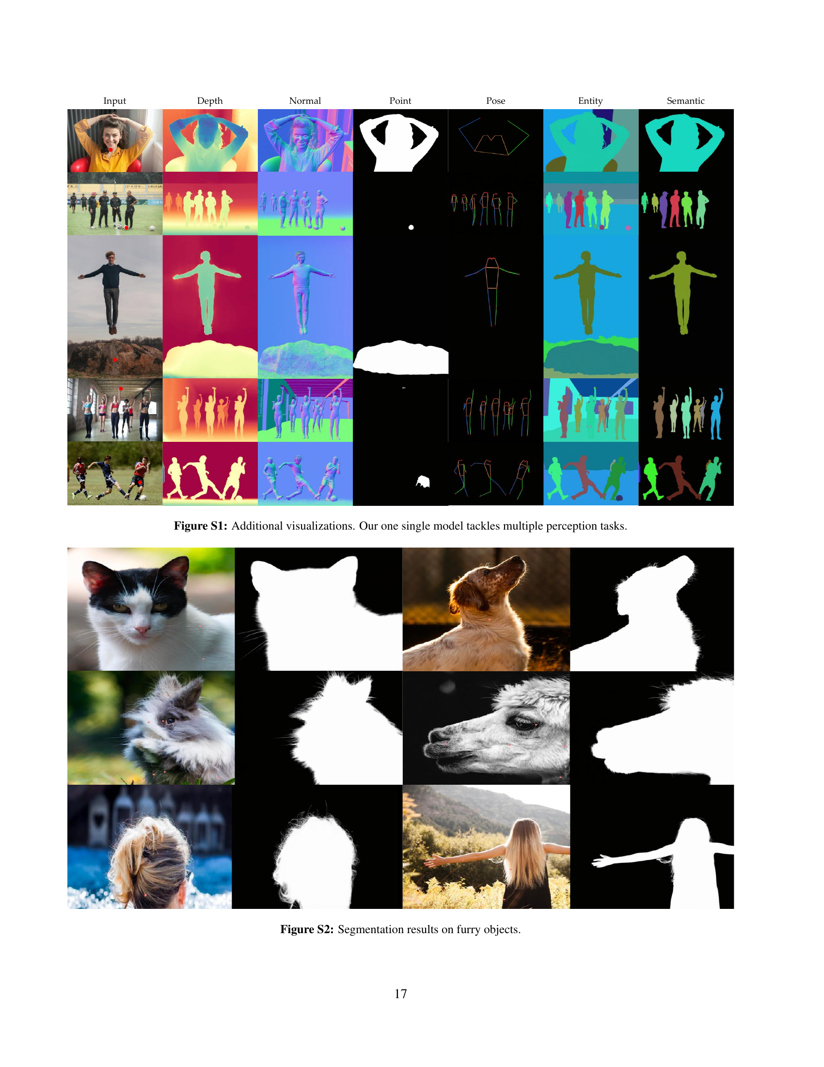
🔼 Figure 1 showcases DiCeption’s capabilities in handling various visual perception tasks. The figure demonstrates that a single DiCeption model can perform multiple tasks (rows 1-3) without needing task-specific components. Point-prompted segmentation is highlighted with red dots as input (rows 1-3). The model’s precision is evident in preserving fine details like hair (row 4). The versatility of the model extends to human pose estimation and semantic segmentation (rows 5-6). Finally, its adaptability is shown by its ability to learn new tasks with minimal fine-tuning (less than 1% of parameters on just 50 images, row 7). Additional results are available in the appendix (Figures S1-S14).
read the caption
Figure 1: With one single model, DiCeption solves multiple tasks without relying on any task-specific modules (rows 1 to 3). The red dots in the figure indicate the input points used for point-prompted segmentation. DiCeption preserves fine details in segmentation, such as hair (row 4). DiCeption supports both human pose estimation and semantic segmentation (row 5, 6). DiCeption can quickly adapt to new tasks by fine-tuning less than 1% of its parameters on as few as 50 images (row 7). For additional visualizations, please refer to Figures S1, S2, S4, S6, S7, S8, S9, S10, S11, S12, S13, S14 in the Appendix.

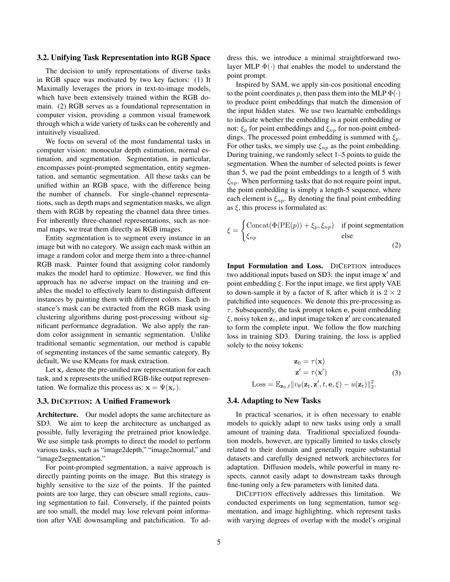
Method	Training	KITTI [32]		NYUv2 [74]		ScanNet [23]		DIODE [102]		ETH3D [92]
Method	Samples	AbsRel $\downarrow$	$\delta_{1}$ $\uparrow$	AbsRel $\downarrow$	$\delta_{1}$ $\uparrow$	AbsRel $\downarrow$	$\delta_{1}$ $\uparrow$	AbsRel $\downarrow$	$\delta_{1}$ $\uparrow$	AbsRel $\downarrow$	$\delta_{1}$ $\uparrow$
MiDaS [86]	2M	0.236	0.630	0.111	0.885	0.121	0.846	0.332	0.715	0.184	0.752
Omnidata [27]	12.2M	0.149	0.835	0.074	0.945	0.075	0.936	0.339	0.742	0.166	0.778
DPT-large [85]	1.4M	0.100	0.901	0.098	0.903	0.082	0.934	0.182	0.758	0.078	0.946
DepthAnything^† [118]	63.5M	0.080	0.946	0.043	0.980	0.043	0.981	0.261	0.759	0.058	0.984
DepthAnything v2^† [119]	62.6M	0.080	0.943	0.043	0.979	0.042	0.979	0.321	0.758	0.066	0.983
Depth Pro^† [7]	-	0.055	0.974	0.042	0.977	0.041	0.978	0.217	0.764	0.043	0.974
Metric3D v2^† [43]	16M	0.052	0.979	0.039	0.979	0.023	0.989	0.147	0.892	0.040	0.983
DiverseDepth [125]	320K	0.190	0.704	0.117	0.875	0.109	0.882	0.376	0.631	0.228	0.694
LeReS [126]	354K	0.149	0.784	0.090	0.916	0.091	0.917	0.271	0.766	0.171	0.777
HDN [128]	300K	0.115	0.867	0.069	0.948	0.080	0.939	0.246	0.780	0.121	0.833
GeoWizard [31]	280K	0.097	0.921	0.052	0.966	0.061	0.953	0.297	0.792	0.064	0.961
DepthFM [33]	63K	0.083	0.934	0.065	0.956	-	-	0.225	0.800	-	-
Marigold^† [47]	74K	0.099	0.916	0.055	0.964	0.064	0.951	0.308	0.773	0.065	0.960
DMP Official^† [54]	-	0.240	0.622	0.109	0.891	0.146	0.814	0.361	0.706	0.128	0.857
GeoWizard^† [31]	280K	0.129	0.851	0.059	0.959	0.066	0.953	0.328	0.753	0.077	0.940
DepthFM^† [33]	63K	0.174	0.718	0.082	0.932	0.095	0.903	0.334	0.729	0.101	0.902
Genpercept^† [114]	90K	0.094	0.923	0.091	0.932	0.056	0.965	0.302	0.767	0.066	0.957
Painter^† [109]	24K	0.324	0.393	0.046	0.979	0.083	0.927	0.342	0.534	0.203	0.644
Unified-IO^† [69]	48K	0.188	0.699	0.059	0.970	0.063	0.965	0.369	0.906	0.103	0.906
4M-XL^† [72]	759M	0.105	0.896	0.068	0.951	0.065	0.955	0.331	0.734	0.070	0.953
OneDiffusion^† [53]	500K	0.101	0.908	0.087	0.924	0.094	0.906	0.399	0.661	0.072	0.949
Ours-single^†	500K	0.081	0.942	0.068	0.949	0.078	0.945	0.267	0.709	0.059	0.969
Ours^†	500K	0.075	0.945	0.072	0.939	0.075	0.938	0.243	0.741	0.053	0.967

🔼 Table 1 presents a quantitative comparison of depth estimation methods, evaluating both specialized models designed for a single task and multi-task models capable of handling multiple tasks simultaneously. The evaluation is performed on zero-shot datasets, meaning the models are tested on data they haven’t seen during training. This assesses the models’ generalization capabilities. The table compares various metrics (AbsRel, 81, etc.) across different datasets (KITTI, NYUv2, ScanNet, etc.). The results demonstrate that the proposed visual generalist model achieves performance comparable to state-of-the-art specialized models, highlighting its effectiveness in depth estimation without task-specific training. The evaluation protocol used is consistent with the Genpercept method.
read the caption
Table 1: Quantitative comparison of depth estimation with both specialized models and multi-task models on zero-shot datasets. Our visual generalist model can perform on par with state-of-the-art models. We use the same evaluation protocal (††\dagger†) as Genpercept [114].

In-depth insights
#

Diffusion Prior
#

Diffusion priors, stemming from the success of diffusion models in generative tasks, offer a powerful inductive bias for various computer vision problems. Their ability to generate realistic and diverse samples suggests a strong learned representation of the visual world, which can be leveraged for tasks beyond generation. Instead of training models from scratch, initializing with or incorporating a diffusion prior allows for faster convergence, better generalization, and reduced data requirements. This is especially beneficial in data-scarce scenarios or when dealing with complex tasks where learning from scratch is challenging. By utilizing the inherent knowledge encoded in diffusion models, researchers can effectively transfer this knowledge to downstream tasks, achieving state-of-the-art results with significantly less computational resources. Moreover, diffusion priors enable the exploration of novel architectures and training strategies, opening up new possibilities for solving long-standing problems in computer vision.

RGB Task Unifier
#

The concept of an ‘RGB Task Unifier’ is intriguing, suggesting a system where various visual tasks are represented and processed within the RGB color space. This unification could have several benefits. Firstly, it could simplify the architecture by providing a common input/output format, potentially reducing the need for task-specific modules. Secondly, leveraging the RGB space might allow the model to exploit pre-trained knowledge from image datasets, as most vision models are trained on RGB images. However, this approach also presents challenges. Encoding diverse tasks like depth estimation or semantic segmentation into RGB might lead to information loss or require complex encoding schemes. Also, the interpretability of the RGB representation could be an issue, making it difficult to understand the model’s reasoning process. Ultimately, the success of an RGB Task Unifier hinges on effectively balancing the simplicity and expressiveness of the RGB representation, ensuring it can capture the nuances of different visual tasks without sacrificing performance.

Data-Efficient
#

In the context of deep learning and computer vision, “Data-Efficient” methods are highly valuable. The ability to achieve high performance with limited data has huge practical implications. Data scarcity is a common bottleneck in real-world applications. Data-efficient techniques often rely on strategies like transfer learning, leveraging pre-trained models on large datasets and fine-tuning on smaller task-specific sets. Meta-learning, or learning to learn, is another approach, enabling models to quickly adapt to new tasks with few examples. Other methods include data augmentation techniques, synthetic data generation, and self-supervised learning.

Few-Shot Adapt
#

Few-shot adaptation is a crucial capability for generalist models, enabling them to rapidly specialize to new tasks with limited data. Effective few-shot adaptation hinges on leveraging pre-trained knowledge and minimizing the risk of overfitting to the scarce training examples. Strategies such as meta-learning can pre-train a model to be adaptable, while techniques like fine-tuning a small subset of parameters or using LoRA layers, injecting task-specific information can efficiently transfer knowledge. Furthermore, regularization methods and data augmentation become vital to prevent overfitting. Success in few-shot adaptation highlights the model’s ability to abstract underlying task structures and its robustness to distribution shifts.

Mask Refinement
#

Mask refinement is a critical step in various computer vision tasks, especially segmentation. It focuses on improving the quality and accuracy of initially predicted masks. Techniques often involve morphological operations to fill holes or remove noise. Edge refinement methods are applied to improve boundary details. Also, using Conditional Random Fields (CRFs) to model relationships between pixels to enforce smoothness and consistency. Deep learning approaches use specialized layers for boundary enhancement or iterative refinement networks to progressively refine masks. The choice of refinement technique depends on the specific task, dataset, and the characteristics of initial masks, with the goal of creating more precise and visually plausible segmentations. In short, refining masks lead to better segmentation.

More visual insights
#

More on figures

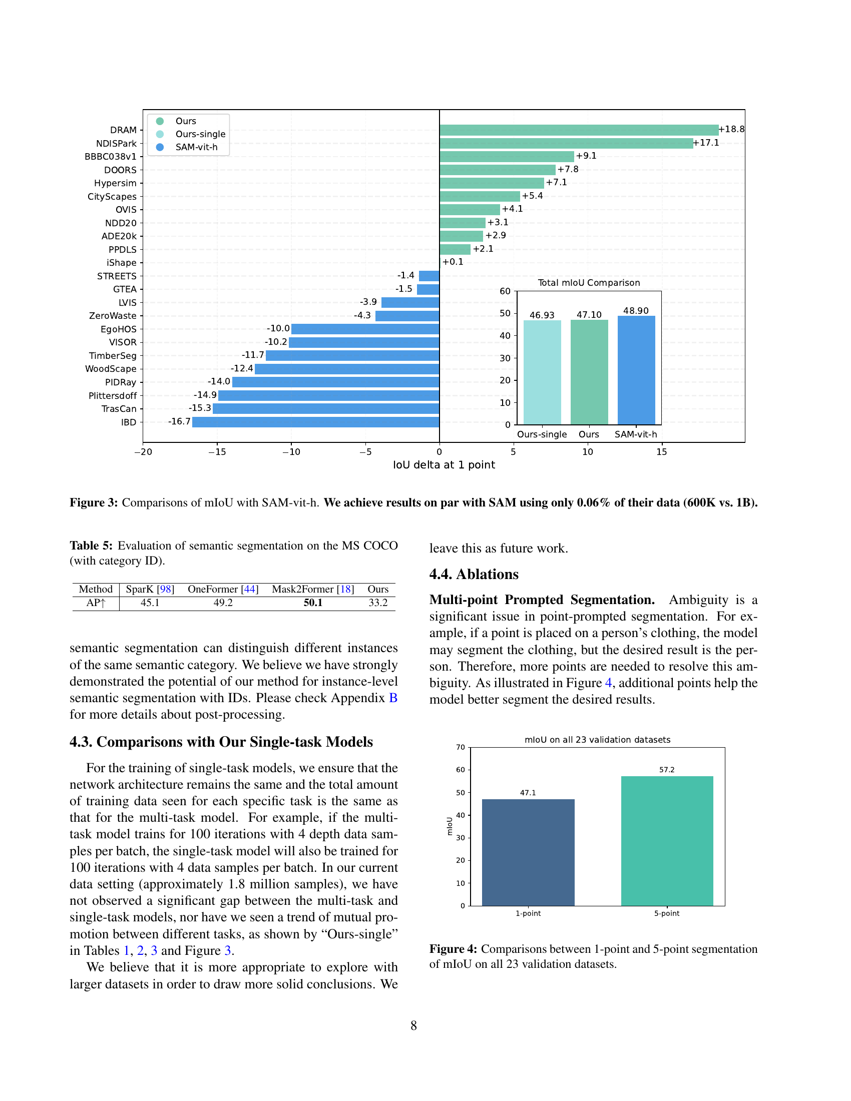
🔼 This figure presents a bar chart comparing the mean Intersection over Union (mIoU) scores achieved by the DICEPTION model and the SAM-vit-h model on various datasets. The key finding is that DICEPTION achieves comparable performance to SAM-vit-h while using significantly less data – a mere 0.06% of the data used by SAM-vit-h (600,000 images versus 1 billion images). The chart visually represents the difference in mIoU scores for each dataset, highlighting DICEPTION’s efficiency in achieving similar results with drastically reduced data requirements.
read the caption
Figure 2: Comparisons of mIoU with SAM-vit-h. We achieve results on par with SAM using only 0.06% of their data (600K vs. 1B).

🔼 This figure compares the mean Intersection over Union (mIoU) scores achieved by a model using one versus five points in a point-prompted segmentation task. The comparison is performed across all 23 validation datasets used in the study. The goal is to demonstrate how increasing the number of input points can impact the performance and accuracy of the model in segmenting objects.
read the caption
Figure 3: Comparisons between 1-point and 5-point segmentation of mIoU on all 23 validation datasets.

🔼 This figure shows a variety of examples demonstrating the model’s ability to perform multiple visual perception tasks using a single model. Each row represents a different input image and shows the model’s output for depth estimation, surface normal estimation, point-prompted segmentation, pose estimation, entity segmentation, and semantic segmentation. This showcases the versatility of the DICEPTION model in handling diverse visual perception tasks, even with minimal training data per task.
read the caption
Figure S1: Additional visualizations. Our one single model tackles multiple perception tasks.

🔼 This figure showcases the DICEPTION model’s performance on images containing furry objects, a challenging scenario for segmentation. The results demonstrate the model’s ability to accurately delineate the boundaries of furry animals, such as cats, dogs, and llamas, even in the presence of fine details and variations in fur texture.
read the caption
Figure S2: Segmentation results on furry objects.

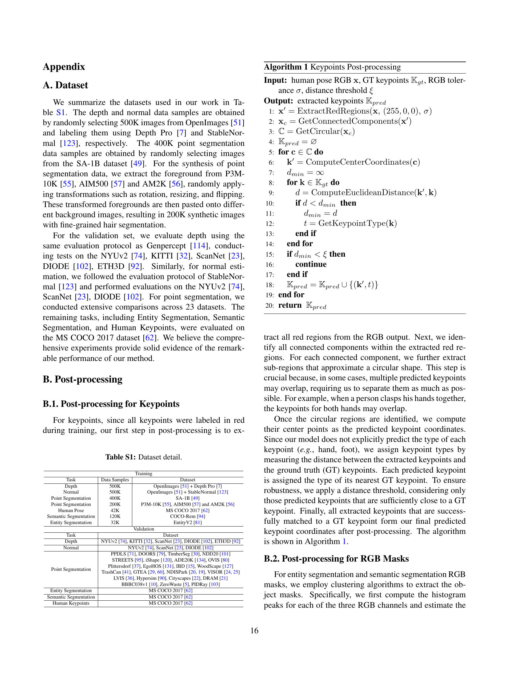
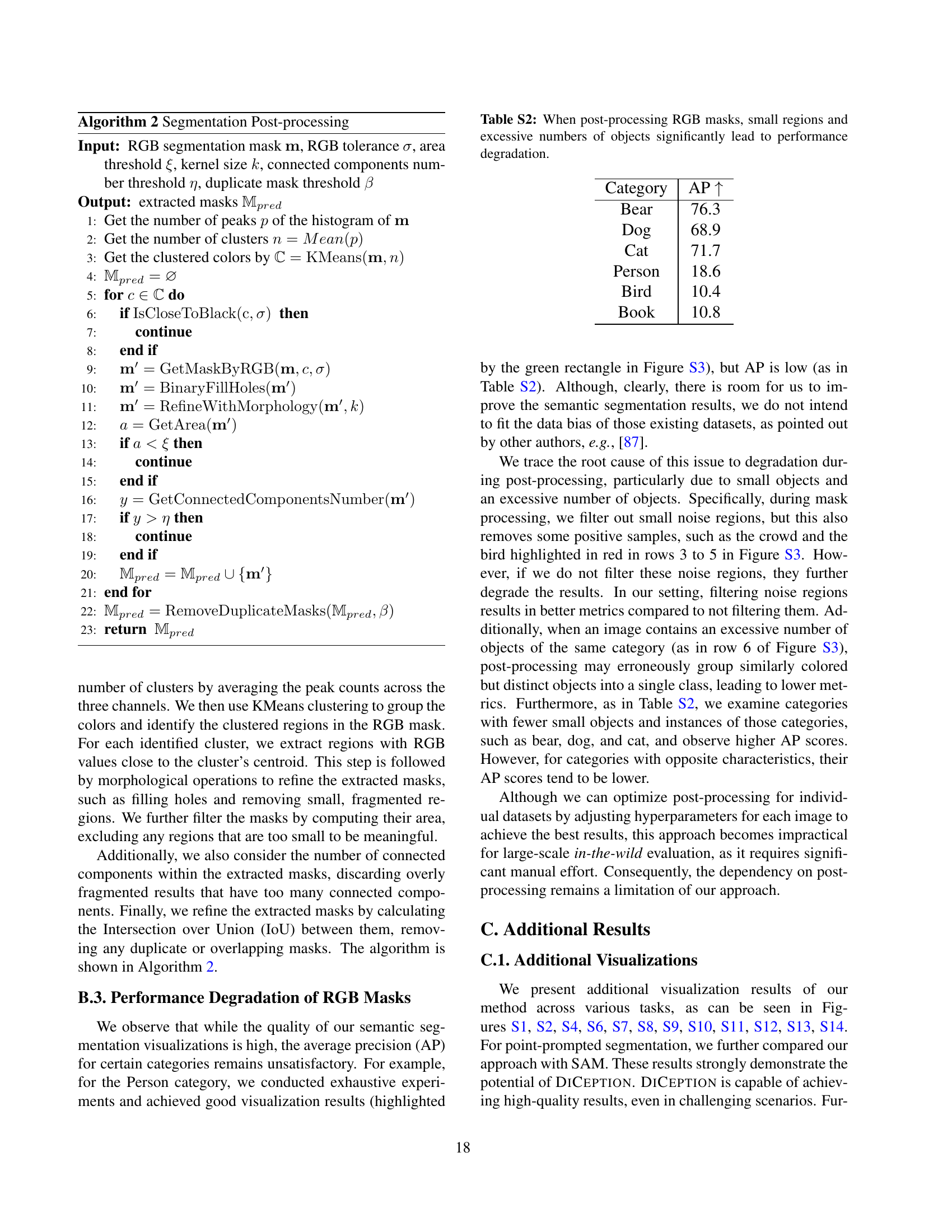
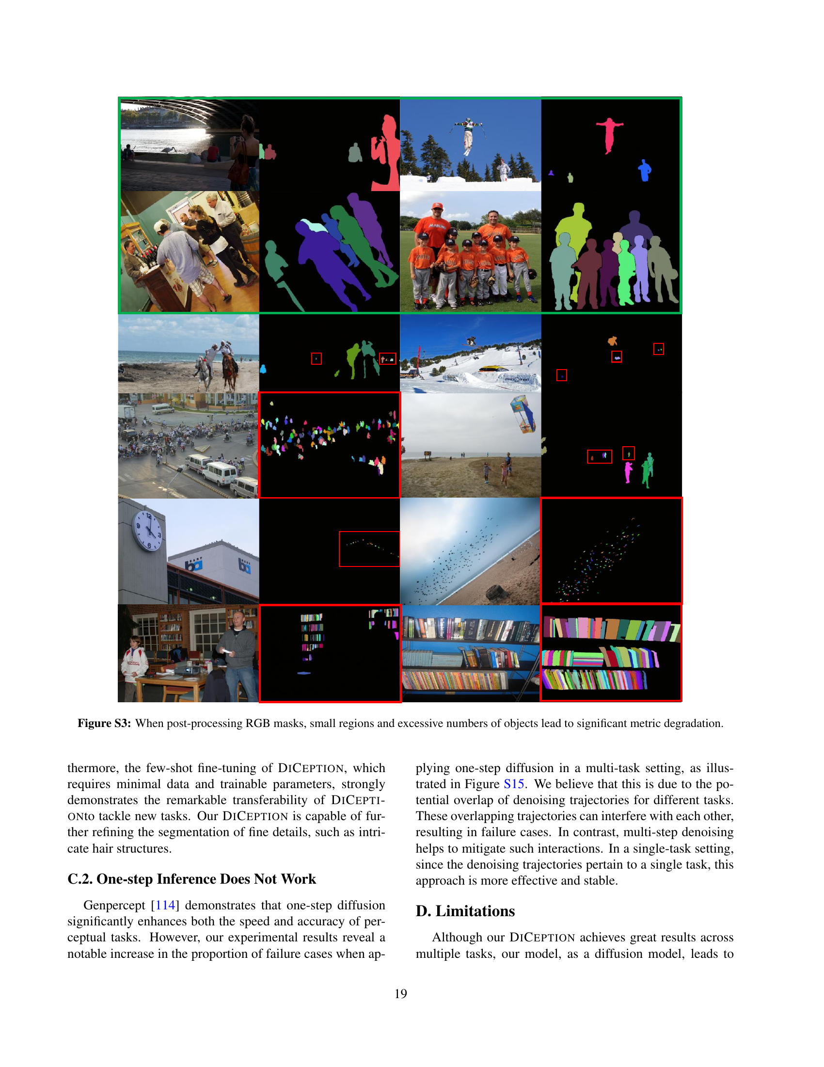
🔼 During post-processing of RGB segmentation masks, the algorithm filters out small regions and those with excessive numbers of objects. While this improves the overall quality, it also removes some valid segments (like small birds or people in a crowd), leading to significant drops in metrics such as average precision (AP). The figure likely shows examples where this filtering negatively impacts the results.
read the caption
Figure S3: When post-processing RGB masks, small regions and excessive numbers of objects lead to significant metric degradation.

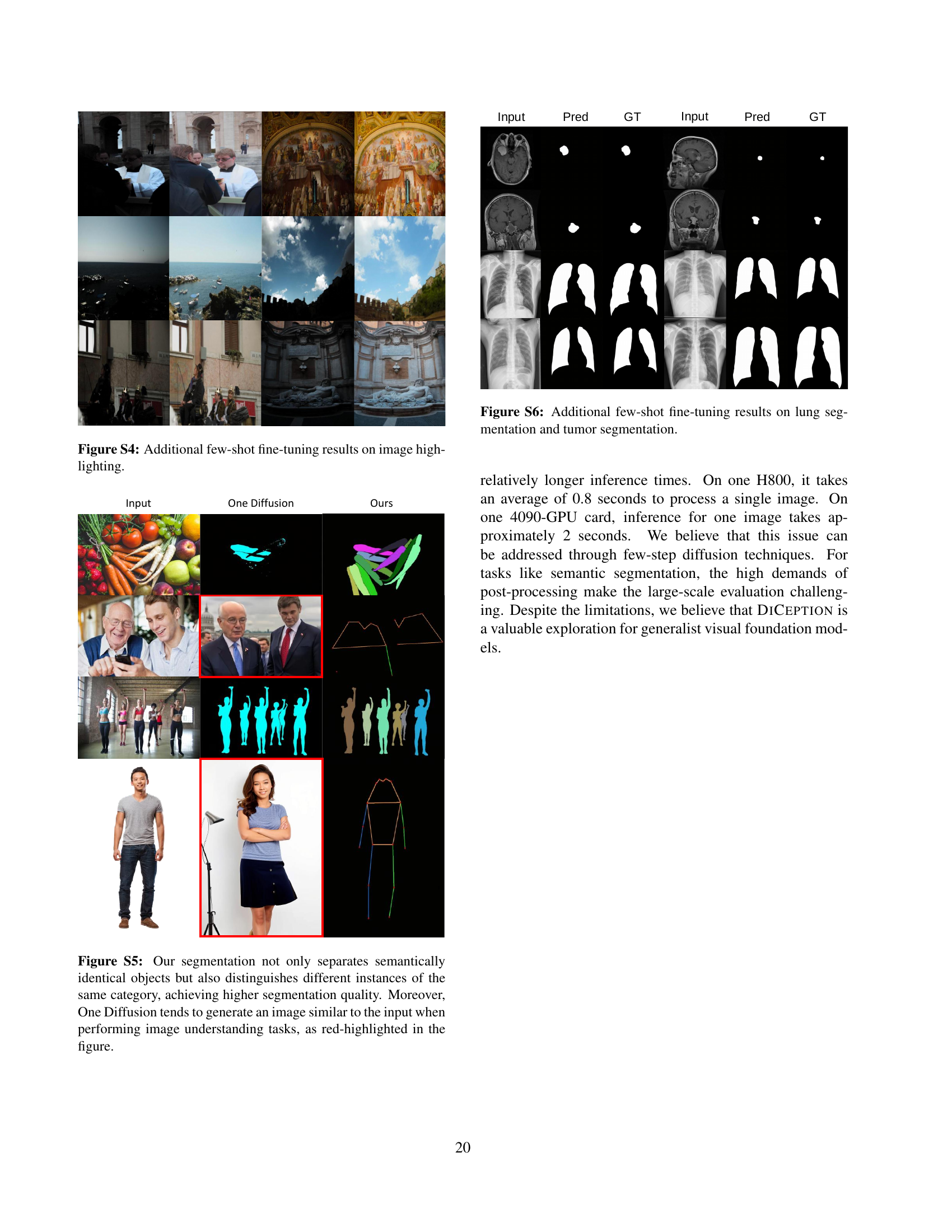
🔼 This figure showcases the results of applying DICEPTION to image highlighting after few-shot fine-tuning. It displays multiple example images where highlighting has been applied to specific regions or objects within the image, demonstrating the model’s ability to adapt quickly to new image manipulation tasks with minimal training data.
read the caption
Figure S4: Additional few-shot fine-tuning results on image highlighting.

🔼 The figure showcases a comparison of DICEPTION’s segmentation results versus One Diffusion’s on various images. DICEPTION effectively differentiates between semantically similar objects and successfully segments multiple instances of the same category, leading to improved segmentation accuracy and detail. In contrast, One Diffusion, when tasked with image understanding, produces output images that closely resemble the input, failing to effectively perform the segmentation task, a shortcoming highlighted by the red boxes in the figure.
read the caption
Figure S5: Our segmentation not only separates semantically identical objects but also distinguishes different instances of the same category, achieving higher segmentation quality. Moreover, One Diffusion tends to generate an image similar to the input when performing image understanding tasks, as red-highlighted in the figure.

🔼 This figure displays the results of fine-tuning DICEPTION on lung and tumor segmentation tasks using a small amount of data. It showcases the model’s ability to adapt quickly to new medical imaging tasks and achieve high-quality segmentations, even with limited training samples. Each image pair likely shows an input medical image and the corresponding segmentation mask produced by DICEPTION after few-shot fine-tuning. The accuracy and detail of the segmentations highlight DICEPTION’s effectiveness.
read the caption
Figure S6: Additional few-shot fine-tuning results on lung segmentation and tumor segmentation.

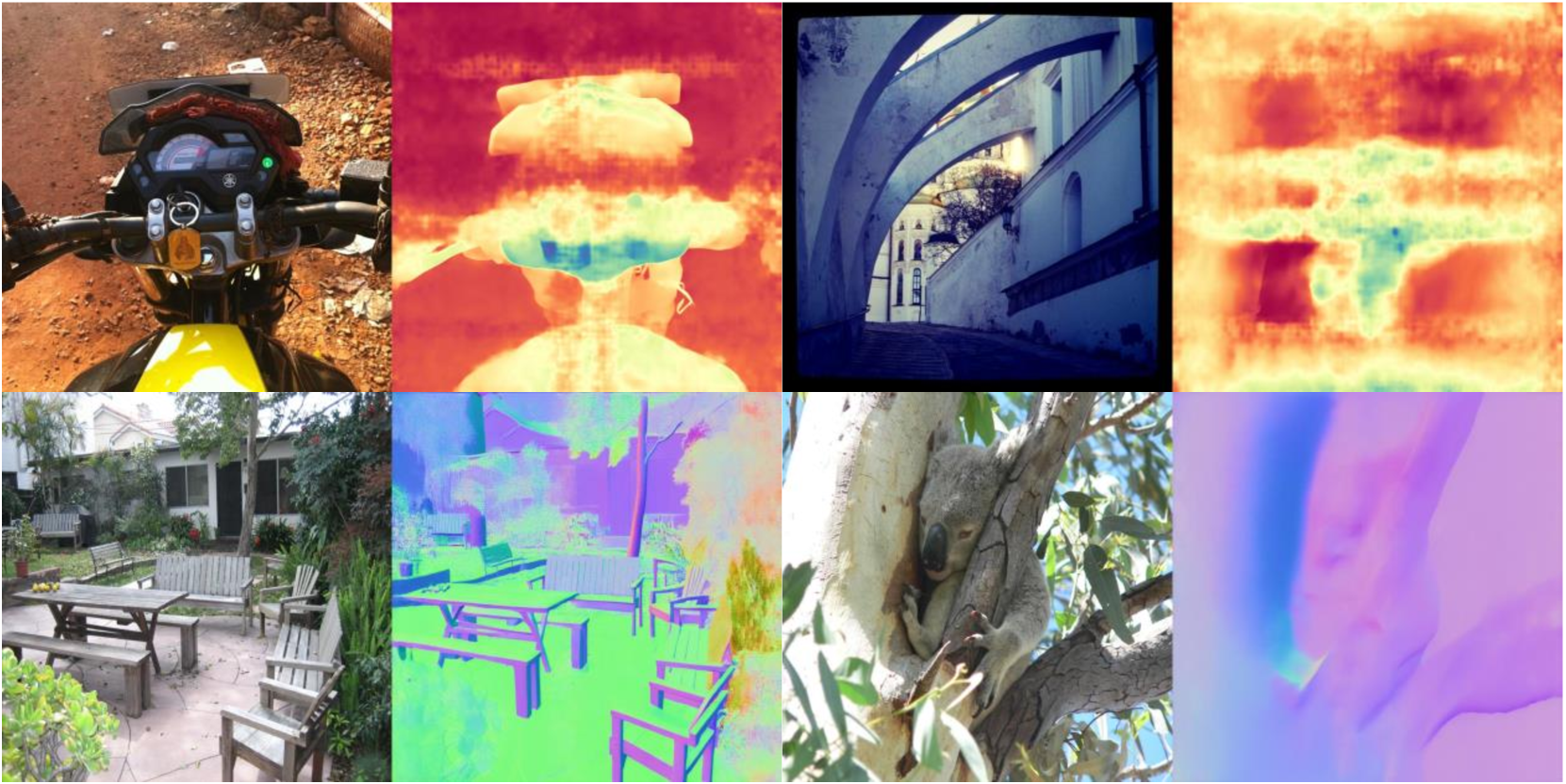
🔼 This figure displays a grid of images, each showing a different scene, along with their corresponding depth estimations generated by the DICEPTION model. The depth maps are presented in a heatmap format, where warmer colors represent closer distances and cooler colors represent further distances. This visualization showcases DICEPTION’s capacity for accurate depth estimation across diverse real-world scenes and objects.
read the caption
Figure S7: Additional depth estimation visualizations.

🔼 This figure displays a grid of images showcasing additional examples of surface normal estimations generated by the DICEPTION model. Surface normals are crucial for representing the 3D shape and orientation of surfaces in images, and this visualization helps demonstrate the model’s ability to accurately estimate these normals across a variety of scenes and objects, including people, cars, furniture, and everyday items.
read the caption
Figure S8: Additional normal visualizations.

🔼 This figure displays a grid of images showcasing the results of entity segmentation performed by the DICEPTION model. Entity segmentation focuses on identifying individual instances within an image without classifying them into specific categories. Each identified instance is assigned a unique random color, facilitating visual distinction between different objects. The images demonstrate the model’s ability to accurately segment diverse objects, ranging from everyday items (like bowls of fruit) to more complex scenes, showcasing the model’s effectiveness across various object types and levels of visual complexity.
read the caption
Figure S9: Additional entity segmentation visualizations.

🔼 This figure displays several examples of point-prompted image segmentation results. Point-prompted segmentation uses a small number of points as input to specify the region of interest for segmentation. The figure showcases the model’s ability to accurately segment diverse objects and scenes, even with complex backgrounds or unusual viewpoints. Each image shows the input image alongside the model’s predicted segmentation mask highlighting the object or area specified by the input points.
read the caption
Figure S10: Additional point-prompted segmentation visualizations.

🔼 This figure displays a comparison of segmentation results between the DiCeption model and the SAM-vit-h model. Both models were given a single point as input to guide the segmentation process. The images show side-by-side comparisons of the input image, DiCeption’s output segmentation mask, and SAM-vit-h’s output segmentation mask. This allows for a visual assessment of the relative performance of the two models on various image types and segmentation challenges using minimal input information.
read the caption
Figure S11: Comparison of the segmentation results between DiCeption and SAM-vit-h with 1-point input.

🔼 This figure displays a comparison of segmentation results obtained using DiCeption and SAM-vit-h. Both models were given the same input images and five points to guide their segmentation. The comparison highlights the differences in segmentation accuracy and detail captured by each model, demonstrating the relative strengths and weaknesses of DiCeption and SAM-vit-h for point-prompted segmentation tasks.
read the caption
Figure S12: Comparison of the segmentation results between DiCeption and SAM-vit-h with 5-point input.

🔼 This figure displays several example images and their corresponding human pose estimations generated by the DICEPTION model. The images show diverse scenes and poses, demonstrating the model’s ability to accurately estimate human poses in various contexts. Each image is paired with a visualization of the detected keypoints and their connections, illustrating the model’s performance on different individuals, clothing styles, and activities.
read the caption
Figure S13: Additional pose estimation visualizations.

🔼 This figure shows various examples of semantic segmentation results produced by the DICEPTION model. It demonstrates the model’s ability to accurately segment various objects and scenes into their respective semantic classes, showcasing its performance on a range of complex and diverse visual inputs. The images depict a variety of scenes and objects, including food items, landscapes, and indoor settings. Each image has its corresponding ground truth segmentation for comparison. The color-coded segmentation masks illustrate the model’s classification of different semantic categories within the scene.
read the caption
Figure S14: Additional semantic segmentation visualizations.

🔼 The figure shows examples where using a one-step denoising process in the DICEPTION model, instead of the standard multi-step approach, leads to a significant increase in prediction errors or failures, particularly in more complex visual perception tasks. The one-step method’s inability to properly resolve ambiguity and handle intricate details across multiple tasks simultaneously is highlighted.
read the caption
Figure S15: The model tends to produce more failure cases in 1-step scenario.

🔼 This figure demonstrates the failure of a UNet-based model to effectively handle multiple visual perception tasks simultaneously. Unlike the DICEPTION model (which uses a Transformer-based architecture), the UNet architecture struggles to maintain comprehensive representations across various tasks, leading to significantly reduced performance and an inability to achieve good results on multiple tasks concurrently. This highlights the limitations of the UNet structure for multi-task learning in comparison to the more capable Transformer-based architecture.
read the caption
Figure S16: A UNet-based model fails to perform multi-task.

More on tables

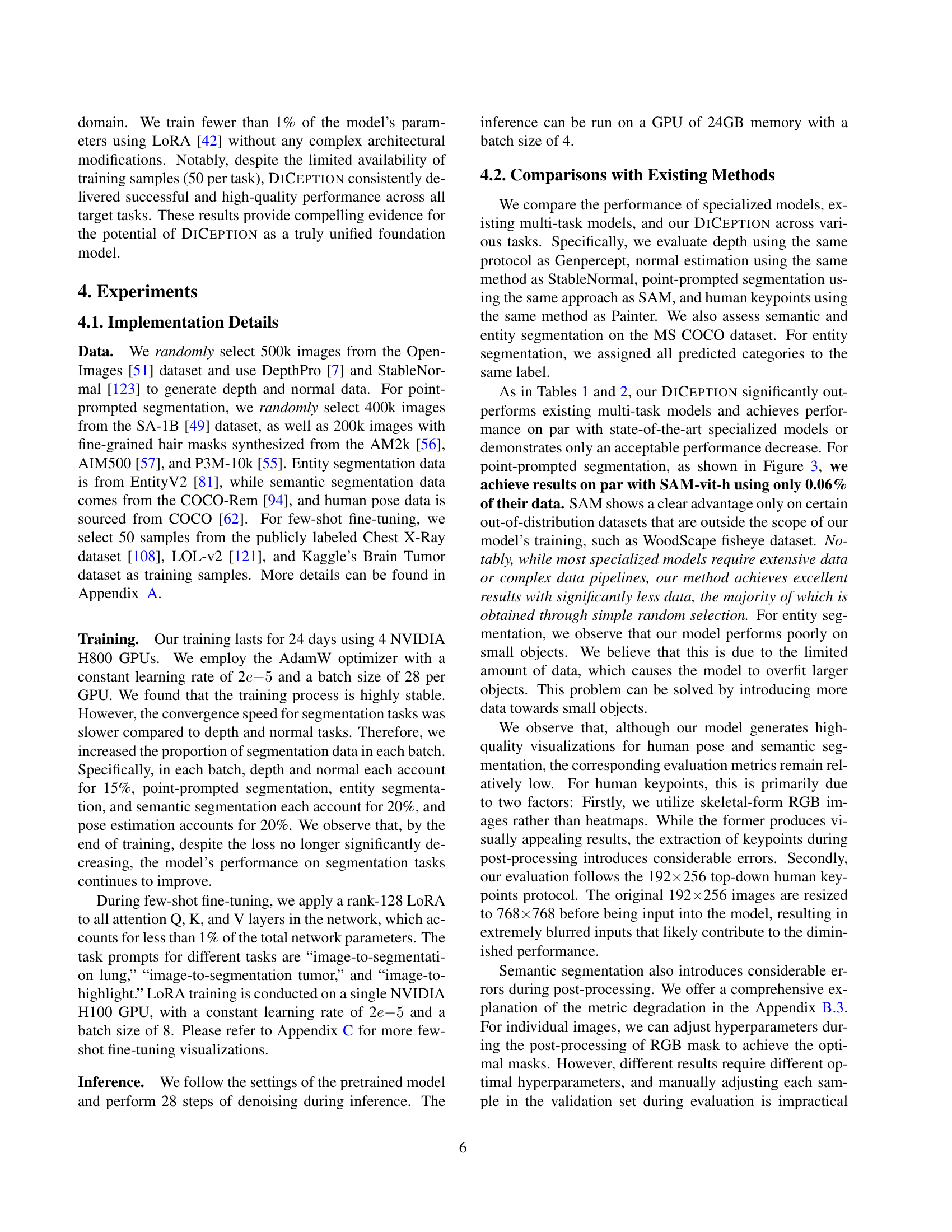
Method	Training	NYUv2 [74]					ScanNet [23]					DIODE-indoor [102]
Method	Samples	mean $\downarrow$	med $\downarrow$	$11.25^{\circ}$ $\uparrow$	$22.5^{\circ}$ $\uparrow$	$30^{\circ}$ $\uparrow$	mean $\downarrow$	med $\downarrow$	$11.25^{\circ}$ $\uparrow$	$22.5^{\circ}$ $\uparrow$	$30^{\circ}$ $\uparrow$	mean $\downarrow$	med $\downarrow$	$11.25^{\circ}$ $\uparrow$	$22.5^{\circ}$ $\uparrow$	$30^{\circ}$ $\uparrow$
DINSE [3]	160K	18.572	10.845	54.732	74.146	80.256	18.610	9.885	56.132	76.944	82.606	18.453	13.871	36.274	77.527	86.976
Geowizard [31]	280K	20.363	11.898	46.954	73.787	80.804	19.748	9.702	58.427	77.616	81.575	19.371	15.408	30.551	75.426	86.357
GenPercept [114]	90K	20.896	11.516	50.712	73.037	79.216	18.600	8.293	64.697	79.329	82.978	18.348	13.367	39.178	79.819	88.551
Marigold [47]	90K	20.864	11.134	50.457	73.003	79.332	18.463	8.442	64.727	79.559	83.199	16.671	12.084	45.776	82.076	89.879
StableNormal [123]	250K	19.707	10.527	53.042	75.889	81.723	17.248	8.057	66.655	81.134	84.632	13.701	9.460	63.447	86.309	92.107
Painter [109]	-	-	-	-	-	-	-	-	-	-	-	-	-	-	-	-
One Diffusion [53]	-	-	-	-	-	-	-	-	-	-	-	-	-	-	-	-
Unified-IO [68]	210K	28.547	14.637	39.907	63.912	71.240	17.955	10.269	54.120	77.617	83.728	31.576	16.615	27.855	64.973	73.445
4M-XL [72]	759M	37.278	13.661	44.660	60.553	65.327	30.700	11.614	48.743	68.867	73.623	18.189	12.979	36.622	81.844	87.050
Ours-single	500K	18.267	10.238	52.393	76.802	83.113	19.892	12.424	45.930	74.341	81.965	17.611	8.912	62.030	80.827	86.474
Ours	500K	18.302	10.538	52.533	75.977	82.573	19.348	12.129	46.410	74.805	82.176	17.946	8.686	62.641	81.152	85.398

🔼 This table presents a quantitative comparison of surface normal estimation methods. It contrasts the performance of specialized models (designed solely for surface normal estimation) against multi-task models (capable of handling various vision tasks, including surface normal estimation). All methods in the comparison were evaluated using the same StableNormal [123] evaluation protocol, ensuring a consistent and fair comparison. The results are presented in terms of metrics which are not specified in the caption.
read the caption
Table 2: Quantitative comparison of surface normal estimation with both specialized models and multi-task models. All methods are evaluated with the same evaluation protocol of StableNormal [123].

Method	AR-small $\uparrow$	AR-medium $\uparrow$	AR-large $\uparrow$
EntityV2 [81]	0.313	0.551	0.683
Ours-single	0.123	0.424	0.648
Ours	0.121	0.439	0.637

🔼 This table presents a quantitative evaluation of the DICEPTION model’s performance on entity segmentation. Specifically, it shows the average recall (AR) achieved by DICEPTION across different object size categories (small, medium, and large) on the MS COCO validation set. Average recall is a common metric used to assess the ability of a model to correctly identify all instances of objects within an image, taking into account the varying sizes of the objects. Higher AR values indicate better performance.
read the caption
Table 3: Average recall (AR) of entity segmentation on the MS COCO validation set.

	HRNet[96]	HRFormer[129]	ViTPose[115]	Painter[109]	Ours
AP $\uparrow$	76.3	77.2	78.3	72.5	57.8

🔼 This table presents a quantitative comparison of different models’ performance on the MS COCO dataset for the task of human keypoint estimation. The results show the Average Recall (AR) of each model across different keypoint sizes (small, medium, large). This metric assesses how accurately the models detect human keypoints in images.
read the caption
Table 4: Evaluation of human keypoints estimation on MS COCO.

Method	SparK [98]	OneFormer [44]	Mask2Former [18]	Ours
AP $\uparrow$	45.1	49.2	50.1	33.2

🔼 This table presents a quantitative comparison of semantic segmentation performance on the MS COCO dataset. It shows the average precision (AP) achieved by different methods, including the proposed DICEPTION model and several other state-of-the-art models. The ‘with category ID’ specification indicates that the evaluation considers the specific categories of objects present in the segmentation masks, offering a more precise measure of performance than simply evaluating overall pixel-level accuracy.
read the caption
Table 5: Evaluation of semantic segmentation on the MS COCO (with category ID).

Training
Task	Data Samples	Dataset
Depth	500K	OpenImages [51] + Depth Pro [7]
Normal	500K	OpenImages [51] + StableNormal [123]
Point Segmentation	400K	SA-1B [49]
Point Segmentation	200K	P3M-10K [55], AIM500 [57] and AM2K [56]
Human Pose	42K	MS COCO 2017 [62]
Semantic Segmentation	120K	COCO-Rem [94]
Entity Segmentation	32K	EntityV2 [81]
Validation
Task	Dataset
Depth	NYUv2 [74], KITTI [32], ScanNet [23], DIODE [102], ETH3D [92]
Normal	NYUv2 [74], ScanNet [23], DIODE [102]
Point Segmentation	PPDLS [71], DOORS [79], TimberSeg [30], NDD20 [101]
	STREETS [95], iShape [120], ADE20K [134], OVIS [80]
	Plittersdorf [37], EgoHOS [131], IBD [15], WoodScape [127]
	TrashCan [41], GTEA [29, 60], NDISPark [20, 19], VISOR [24, 25]
	LVIS [36], Hypersim [90], Cityscapes [22], DRAM [21]
	BBBC038v1 [10], ZeroWaste [5], PIDRay [103]
Entity Segmentation	MS COCO 2017 [62]
Semantic Segmentation	MS COCO 2017 [62]
Human Keypoints	MS COCO 2017 [62]

🔼 Table S1 provides a detailed breakdown of the datasets used in the DICEPTION research. It lists various datasets employed for different tasks, including the number of samples used for each task and the specific tasks they were used for. The datasets are categorized into training and validation sets, clearly indicating their roles in model training and evaluation. This table allows readers to comprehensively understand the data used for training and evaluating the performance of DICEPTION on different vision perception tasks.
read the caption
Table S1: Dataset detail.

Category	AP $\uparrow$
Bear	76.3
Dog	68.9
Cat	71.7
Person	18.6
Bird	10.4
Book	10.8

🔼 During post-processing of RGB masks generated for semantic and entity segmentation tasks, certain factors significantly impact performance. Small segmented regions might be filtered out as noise, leading to missed objects. Conversely, an excessive number of objects in a single image can cause similar-colored objects to be incorrectly grouped, reducing accuracy. This table shows how the average precision (AP) metric is affected by these issues for various object categories, highlighting that performance suffers when these issues occur.
read the caption
Table S2: When post-processing RGB masks, small regions and excessive numbers of objects significantly lead to performance degradation.

TL;DR#

Key Takeaways#

Why does it matter?#

Visual Insights#

In-depth insights#

Diffusion Prior#

RGB Task Unifier#

Data-Efficient#

Few-Shot Adapt#

Mask Refinement#

More visual insights#

Full paper#