TL;DR#
Rendering dynamic scenes from videos is challenging due to complex motions and need for real-time processing. Deformable Gaussian Splatting shows promise, but suffers from redundant Gaussians leading to slower speeds. Static areas don’t need attribute updates leading to unnecessary processing overhead. The primary bottleneck in rendering speed is the number of Gaussians.
This paper introduces Efficient Dynamic Gaussian Splatting (EDGS) to represent dynamic scenes via sparse time-variant attribute modeling. It formulates dynamic scenes using a sparse anchor-grid with motion flow calculated via kernel representation. It efficiently filters out static area anchors, inputting only deformable object anchors into MLPs for time-variant attribute queries.
Key Takeaways#
Why does it matter?#
This work introduces an efficient approach to dynamic scene rendering, crucial for VR/AR applications. The method significantly improves rendering speed while maintaining quality, addressing a key bottleneck in the field and opening new avenues for real-time dynamic scene reconstruction.
Visual Insights#

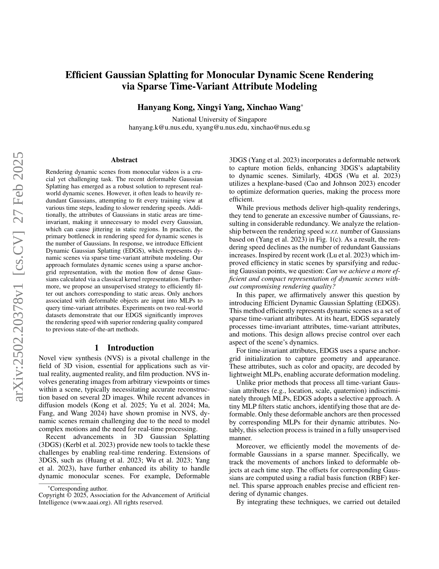
🔼 Figure 1 demonstrates the performance of the proposed method, Efficient Dynamic Gaussian Splatting (EDGS), for rendering dynamic scenes. (a) showcases real-time rendering results with high quality from monocular multi-view images. (b) compares EDGS against other state-of-the-art methods in terms of rendering speed, quality (PSNR), and the number of Gaussians used, highlighting EDGS’s efficiency. The circle’s radius represents the count of time-variant Gaussians whose attributes require querying from MLPs, indicating the computational cost. (c) illustrates the strong correlation between rendering speed and the number of Gaussians, emphasizing that EDGS’s reduced Gaussian count leads to faster rendering.
read the caption
Figure 1: (a) Given a set of monocular multi-view images and camera poses, our method achieves real-time rendering for dynamic scenes while maintaining high rendering quality. (b) Our method achieves promising rendering quality with faster rendering speed and fewer Gaussians. The radius of the circle is the number of time-variant Gaussians whose attributes need to be queried by MLPs. (c) The bottleneck of the rendering speed for dynamic scenes is the number of Gaussians. The fewer the number of Gaussians, the faster the rendering speed.
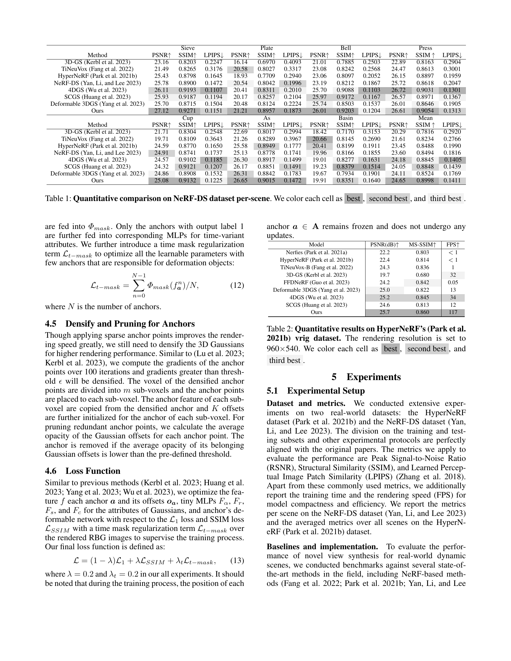
| Method | Sieve | Plate | Bell | Press | ||||||||
| PSNR | SSIM | LPIPS | PSNR | SSIM | LPIPS | PSNR | SSIM | LPIPS | PSNR | SSIM | LPIPS | |
| 3D-GS (Kerbl et al. 2023) | 23.16 | 0.8203 | 0.2247 | 16.14 | 0.6970 | 0.4093 | 21.01 | 0.7885 | 0.2503 | 22.89 | 0.8163 | 0.2904 |
| TiNeuVox (Fang et al. 2022) | 21.49 | 0.8265 | 0.3176 | 20.58 | 0.8027 | 0.3317 | 23.08 | 0.8242 | 0.2568 | 24.47 | 0.8613 | 0.3001 |
| HyperNeRF (Park et al. 2021b) | 25.43 | 0.8798 | 0.1645 | 18.93 | 0.7709 | 0.2940 | 23.06 | 0.8097 | 0.2052 | 26.15 | 0.8897 | 0.1959 |
| NeRF-DS (Yan, Li, and Lee 2023) | 25.78 | 0.8900 | 0.1472 | 20.54 | 0.8042 | 0.1996 | 23.19 | 0.8212 | 0.1867 | 25.72 | 0.8618 | 0.2047 |
| 4DGS (Wu et al. 2023) | 26.11 | 0.9193 | 0.1107 | 20.41 | 0.8311 | 0.2010 | 25.70 | 0.9088 | 0.1103 | 26.72 | 0.9031 | 0.1301 |
| SCGS (Huang et al. 2023) | 25.93 | 0.9187 | 0.1194 | 20.17 | 0.8257 | 0.2104 | 25.97 | 0.9172 | 0.1167 | 26.57 | 0.8971 | 0.1367 |
| Deformable 3DGS (Yang et al. 2023) | 25.70 | 0.8715 | 0.1504 | 20.48 | 0.8124 | 0.2224 | 25.74 | 0.8503 | 0.1537 | 26.01 | 0.8646 | 0.1905 |
| Ours | 27.12 | 0.9271 | 0.1151 | 21.21 | 0.8957 | 0.1873 | 26.01 | 0.9203 | 0.1204 | 26.61 | 0.9054 | 0.1313 |
| Cup | As | Basin | Mean | |||||||||
| Method | PSNR | SSIM | LPIPS | PSNR | SSIM | LPIPS | PSNR | SSIM | LPIPS | PSNR | SSIM | LPIPS |
| 3D-GS (Kerbl et al. 2023) | 21.71 | 0.8304 | 0.2548 | 22.69 | 0.8017 | 0.2994 | 18.42 | 0.7170 | 0.3153 | 20.29 | 0.7816 | 0.2920 |
| TiNeuVox (Fang et al. 2022) | 19.71 | 0.8109 | 0.3643 | 21.26 | 0.8289 | 0.3967 | 20.66 | 0.8145 | 0.2690 | 21.61 | 0.8234 | 0.2766 |
| HyperNeRF (Park et al. 2021b) | 24.59 | 0.8770 | 0.1650 | 25.58 | 0.8949 | 0.1777 | 20.41 | 0.8199 | 0.1911 | 23.45 | 0.8488 | 0.1990 |
| NeRF-DS (Yan, Li, and Lee 2023) | 24.91 | 0.8741 | 0.1737 | 25.13 | 0.8778 | 0.1741 | 19.96 | 0.8166 | 0.1855 | 23.60 | 0.8494 | 0.1816 |
| 4DGS (Wu et al. 2023) | 24.57 | 0.9102 | 0.1185 | 26.30 | 0.8917 | 0.1499 | 19.01 | 0.8277 | 0.1631 | 24.18 | 0.8845 | 0.1405 |
| SCGS (Huang et al. 2023) | 24.32 | 0.9121 | 0.1207 | 26.17 | 0.8851 | 0.1491 | 19.23 | 0.8379 | 0.1514 | 24.05 | 0.8848 | 0.1439 |
| Deformable 3DGS (Yang et al. 2023) | 24.86 | 0.8908 | 0.1532 | 26.31 | 0.8842 | 0.1783 | 19.67 | 0.7934 | 0.1901 | 24.11 | 0.8524 | 0.1769 |
| Ours | 25.08 | 0.9132 | 0.1225 | 26.65 | 0.9015 | 0.1472 | 19.91 | 0.8351 | 0.1640 | 24.65 | 0.8998 | 0.1411 |
🔼 This table presents a quantitative comparison of different novel view synthesis methods on the NeRF-DS dataset. For each scene (Sieve, Plate, Bell, Press, Cup, Basin), the table shows the Peak Signal-to-Noise Ratio (PSNR), Structural Similarity Index (SSIM), and Learned Perceptual Image Patch Similarity (LPIPS) scores achieved by each method. Higher PSNR and SSIM values and lower LPIPS values generally indicate better image quality. The best, second-best, and third-best results for each metric in each scene are highlighted with color-coding for easy comparison.
read the caption
Table 1: Quantitative comparison on NeRF-DS dataset per-scene. We color each cell as best, second best, and third best.
In-depth insights#
Sparse Attribute#
The concept of “Sparse Attribute” modeling centers around representing data or scenes using only a selective subset of attributes, rather than a complete set. This approach acknowledges that not all attributes contribute equally to the underlying structure or dynamic behavior. By identifying and focusing on the most salient attributes, it is possible to achieve a more efficient representation, reducing computational cost and memory footprint. The choice of which attributes to retain or discard is crucial and often relies on domain-specific knowledge or data-driven analysis. Methods for achieving sparsity can include techniques like dimensionality reduction, feature selection, or dictionary learning. Furthermore, sparse attribute modeling often leads to more interpretable models, as the reduced attribute set highlights the key factors influencing the outcome. This sparsity also improves generalization by preventing overfitting to noisy or irrelevant attributes, which is especially useful when dealing with high-dimensional data with limited samples. Efficient algorithms and data structures are essential for processing and manipulating sparse representations, enabling faster computations and improved scalability. The method offers efficiency gains without significantly compromising the accuracy.
Anchor-Grid 3DGS#
Anchor-Grid 3DGS leverages anchor points arranged in a grid to represent the scene’s geometry, offering a structured alternative to directly using Gaussians. This approach provides a compact representation by associating multiple Gaussians with each anchor, which means that only a sparse set of anchors require optimization, greatly reducing computational costs during rendering. Attributes of Gaussians can be efficiently derived from these anchors, with time-invariant properties handled separately from dynamic ones. Furthermore, Anchor-Grid 3DGS allows efficient handling of dynamic scenes by selectively applying deformation only to anchors that are responsible for moving regions, thereby enhancing the rendering speed and reducing jittering in static areas. Such a structured approach allows for better control over the scene’s dynamics and facilitates real-time rendering of high-quality dynamic scenes.
Time-Masked MLPs#
Time-Masked MLPs present an intriguing approach to dynamic scene representation, offering a potential solution to the redundancy often observed in methods like Deformable 3DGS. The core idea is to use a lightweight MLP to identify and filter out static regions within a scene, focusing computational resources on areas undergoing deformation. By processing only the dynamic attributes of deformable objects through MLPs, the approach reduces the overall computational burden, potentially leading to significant improvements in rendering speed. This selective approach contrasts with previous methods that indiscriminately process all time-variant Gaussian attributes, regardless of their actual temporal change. Furthermore, the use of an unsupervised training strategy for the time-mask MLP adds to the elegance and efficiency of the system, eliminating the need for manual labeling or explicit supervision. This strategy can significantly improve the rendering speed of dynamic scenes by reducing the number of Gaussians needed to be processed over time.
RBF Kernel Motion#
The paper leverages a Radial Basis Function (RBF) kernel to model motion, indicating a focus on capturing complex, non-rigid deformations effectively. RBF kernels are known for their ability to model smooth, continuous functions, which is beneficial for representing object movements realistically. By using an RBF kernel, the method likely aims to establish relationships between anchor points and their Gaussian offsets, thereby capturing the dynamic changes in the scene in a sparse and efficient manner. This approach contrasts with methods that directly query Gaussian attributes using deformation networks, potentially leading to redundancy and increased computational cost. The choice of the RBF kernel suggests a preference for smooth motion modeling over strict geometric constraints, enabling the representation of a wider range of dynamic behaviors. Overall, the paper suggests an innovative method for dynamic 3D scene reconstruction that leverages the unique properties of RBF kernels to achieve both accuracy and efficiency.
Dynamic Rendering#
While the provided text doesn’t explicitly use the heading “Dynamic Rendering,” it’s heavily focused on this topic. The research addresses the challenge of rendering dynamic scenes from monocular videos, a complex task requiring accurate modeling of motion and efficient real-time processing. Existing methods, like Deformable 3DGS and 4DGS, struggle with redundant Gaussians, leading to slower rendering speeds. The core issue is the large number of Gaussians needed to fit every training view, and the fact that static areas are unnecessarily remodeled at each time step. The paper introduces Efficient Dynamic Gaussian Splatting (EDGS) as a solution. EDGS uses sparse time-variant attribute modeling. It calculates Gaussian motion through a kernel representation and filters static areas. By focusing only on deformable objects, it reduces redundancy and speeds up rendering without sacrificing quality. The evaluation shows that EDGS achieves faster rendering speeds and superior quality, demonstrating its potential to overcome the limitations of current dynamic scene rendering techniques. In essence, the research explores ways to optimize dynamic rendering, making it more efficient and practical for real-world applications.
More visual insights#
More on figures

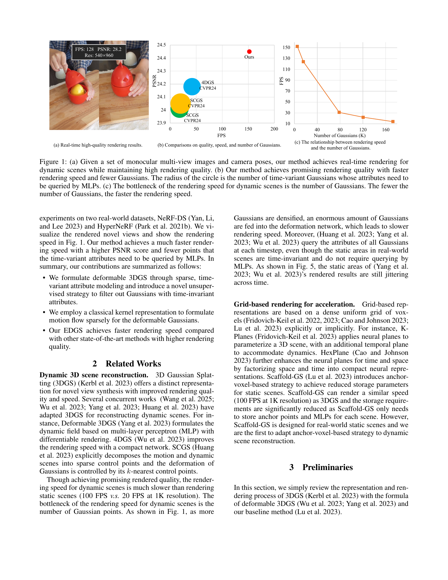
🔼 This figure illustrates the pipeline of Efficient Dynamic Gaussian Splatting (EDGS). It begins by initializing sparse anchor points from a Structure from Motion (SfM) point cloud using COLMAP. A time-mask Multi-Layer Perceptron (MLP) then classifies each anchor point as either static or dynamic. Static anchors receive k Gaussian offsets, and their time-invariant attributes (opacity, quaternion, scale, color) are determined by small MLPs. Dynamic anchors have their time-variant attributes processed by a deformable attribute MLP, with Gaussian locations at each time step calculated using a Radial Basis Function (RBF) kernel to determine the similarity between each Gaussian and its anchor. The entire process is efficient, using small MLPs for attribute calculation and a single network for deformation. Importantly, anchor positions remain fixed.
read the caption
Figure 2: The pipeline of our EDGS. 1) We first initialize voxelized sparse anchor points from Structure from Motion (SfM) points derived from COLMAP. 2) A time-mask MLP is applied to classify if the anchor belongs to the static area or the deformable area. 3) k𝑘kitalic_k Gaussian offsets are initialized for each anchor 𝒂𝒂\bm{a}bold_italic_a belonging to static area. The time-invariant attributes of each Gaussian, i.e., opacity, quaternion, scale, and color are calculated from its feature by corresponding tiny MLPs. 4) Time-variant attributes for anchors from dynamic areas are decoded by a deformable attribute MLP. RBF kernel function is employed to compute the location of each Gaussian at timestep t𝑡titalic_t by calculating the similarity between each Gaussian and its belonging anchor point. This pipeline is compact and efficient, featuring only a few tiny MLPs for the attributes of the Gaussians and a single network for deformations. Notably, the position of each anchor remains static and is not subject to updates.
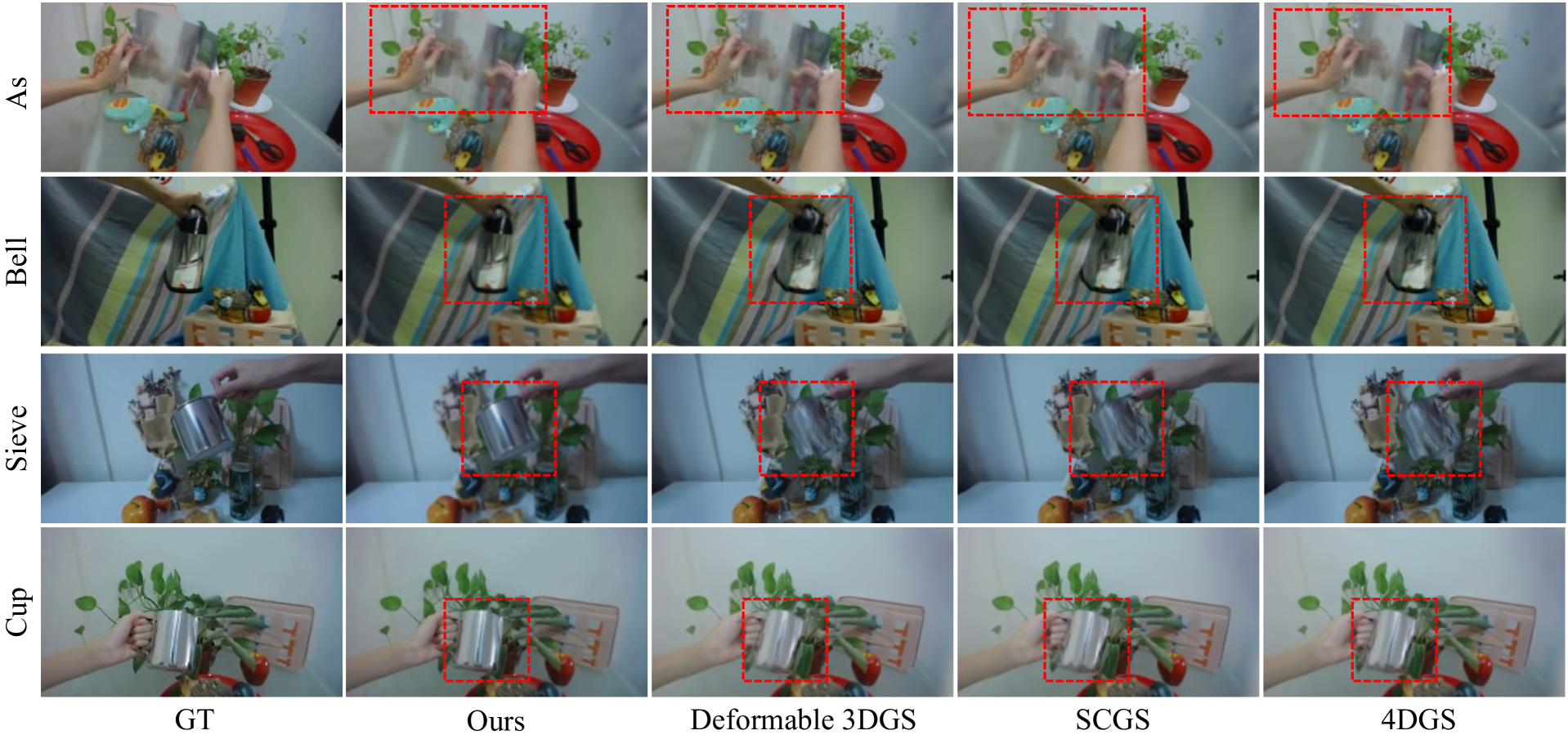
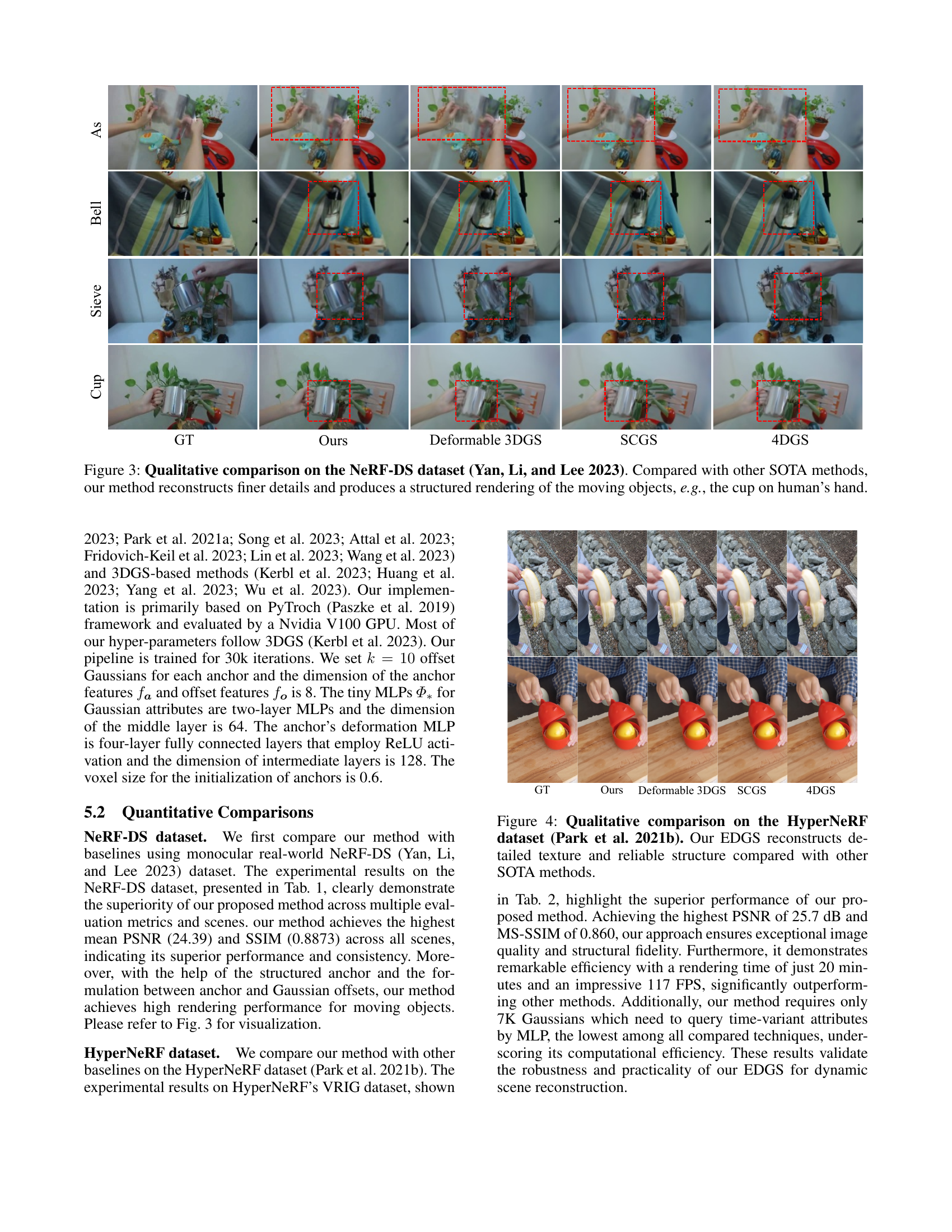
🔼 Figure 3 presents a qualitative comparison of novel view synthesis results on the NeRF-DS dataset. The figure shows how different methods, including the authors’ proposed approach and several state-of-the-art (SOTA) techniques, render a scene containing multiple moving objects. The key takeaway is that the authors’ method reconstructs finer details and achieves more structured rendering of moving elements. This is demonstrated by a comparison of how each method renders a cup held in a hand. The improved detail and structure in the authors’ result indicate a more accurate and visually pleasing representation of the dynamic scene.
read the caption
Figure 3: Qualitative comparison on the NeRF-DS dataset (Yan, Li, and Lee 2023). Compared with other SOTA methods, our method reconstructs finer details and produces a structured rendering of the moving objects, e.g., the cup on human’s hand.
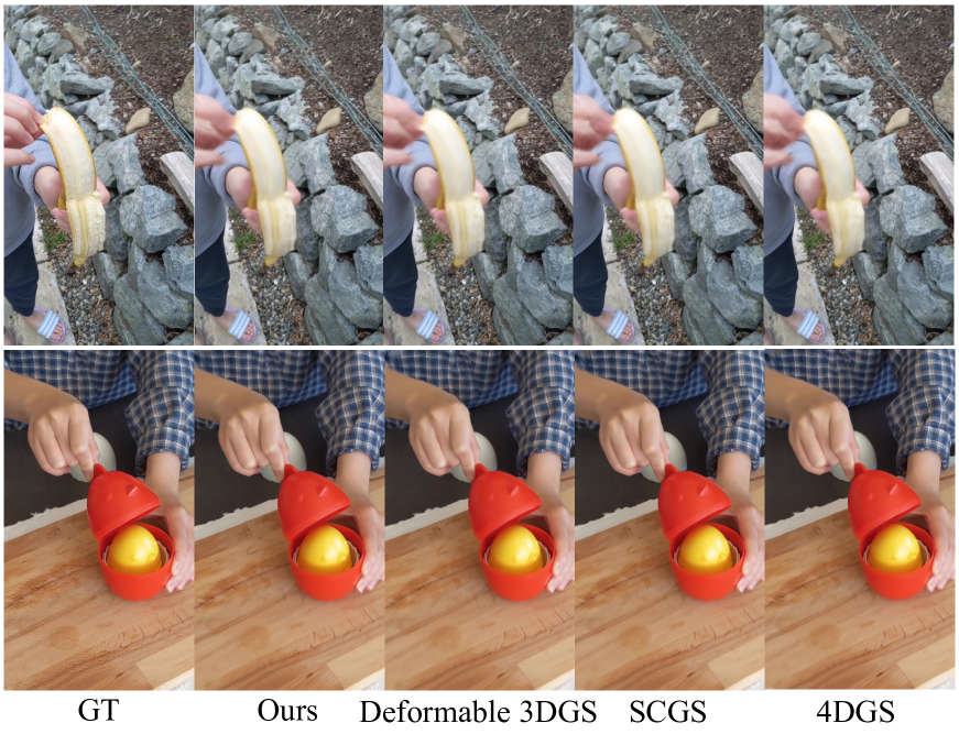
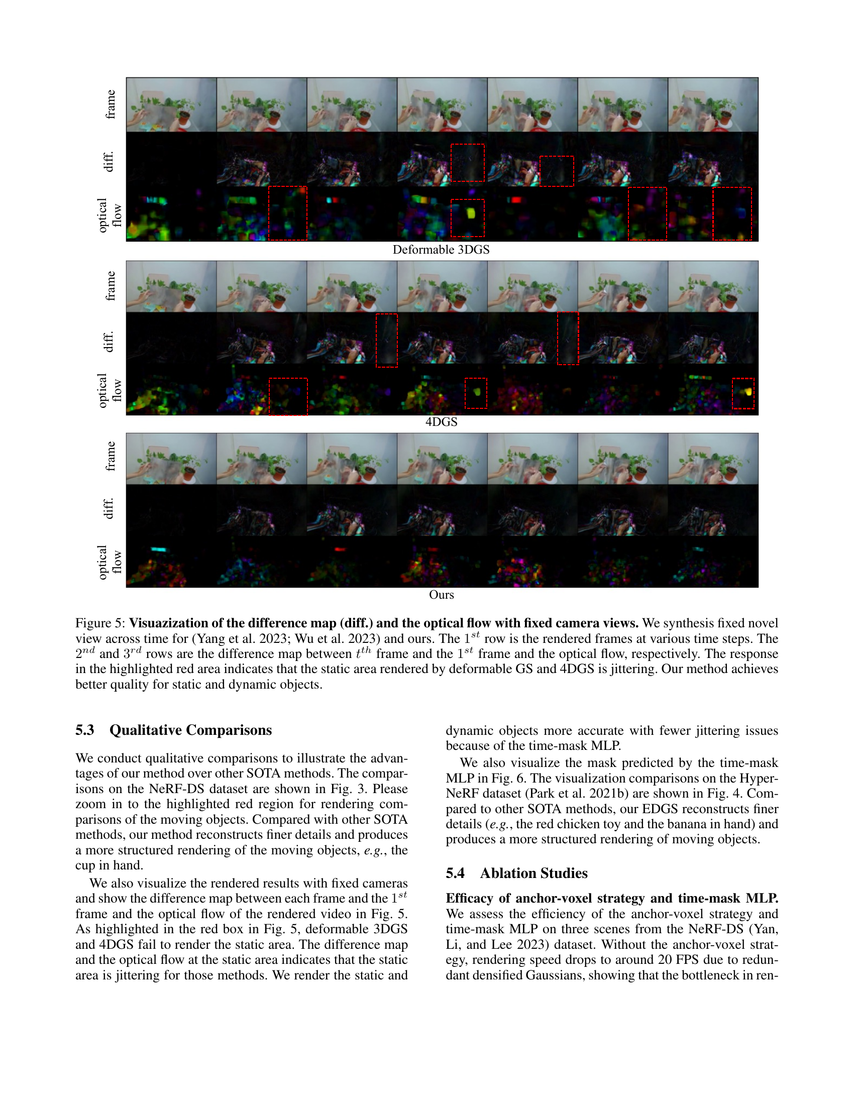
🔼 Figure 4 presents a qualitative comparison of dynamic scene reconstruction results on the HyperNeRF dataset. It visually demonstrates the superior performance of the proposed Efficient Dynamic Gaussian Splatting (EDGS) method against other state-of-the-art (SOTA) techniques. EDGS is shown to reconstruct significantly more detailed textures and a more reliable overall scene structure compared to the other methods. This showcases its ability to capture fine details and accurately represent the scene geometry, even in complex dynamic scenarios.
read the caption
Figure 4: Qualitative comparison on the HyperNeRF dataset (Park et al. 2021b). Our EDGS reconstructs detailed texture and reliable structure compared with other SOTA methods.

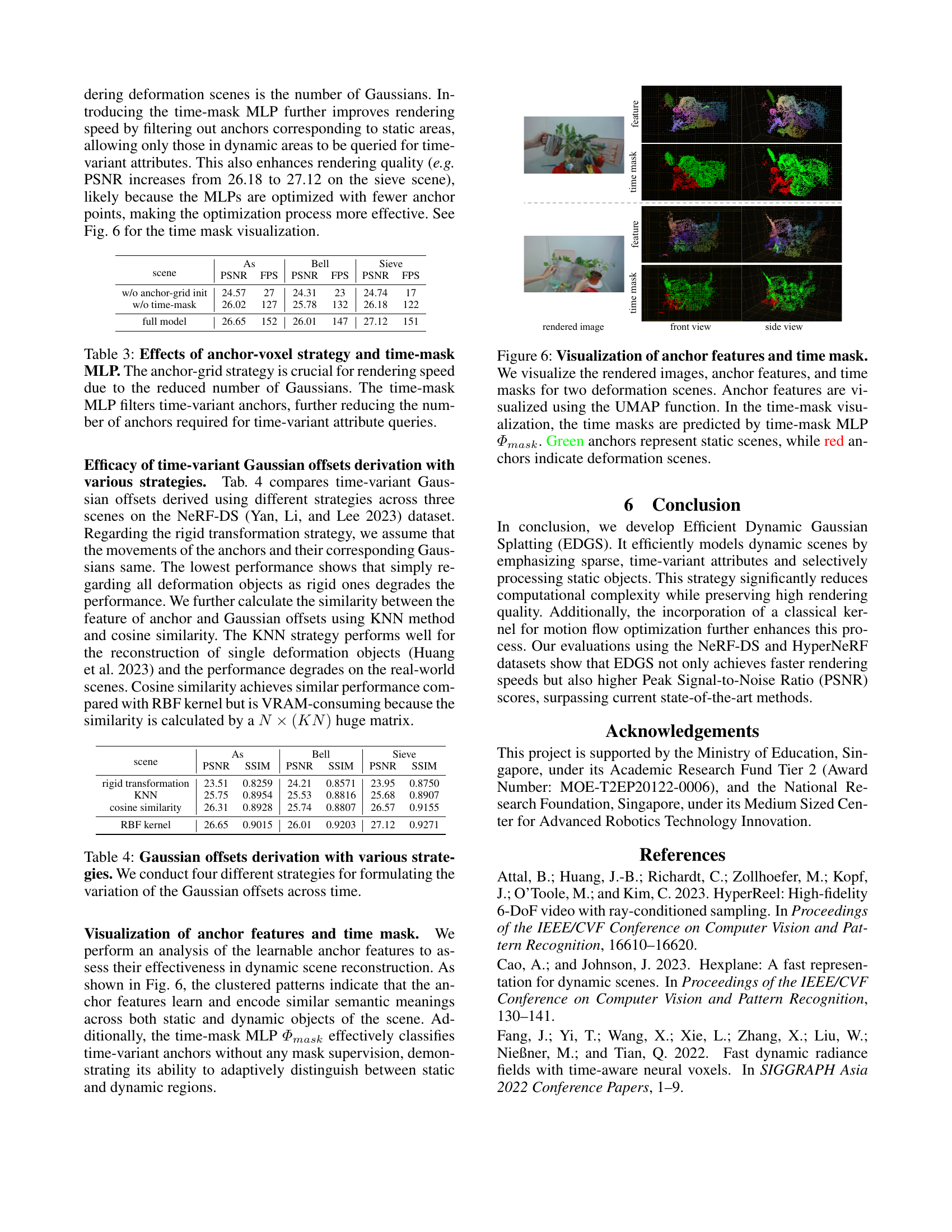
🔼 Figure 5 compares the rendering results of three different methods: Deformable 3DGS, 4DGS, and the proposed method (Ours). It shows three rows of visualizations for each method, all using a fixed camera perspective across several time steps. The top row displays the rendered frames. The second row presents the difference between each frame and the first frame, highlighting changes over time. The third row illustrates the optical flow, showing movement vectors. The red box emphasizes a region where the static elements appear to exhibit jittering (unwanted movement) in Deformable 3DGS and 4DGS, indicating a deficiency in representing these parts of the scene. The authors’ method avoids this issue, resulting in improved quality for both static and dynamic scene elements.
read the caption
Figure 5: Visuazization of the difference map (diff.) and the optical flow with fixed camera views. We synthesis fixed novel view across time for (Yang et al. 2023; Wu et al. 2023) and ours. The 1stsuperscript1𝑠𝑡1^{st}1 start_POSTSUPERSCRIPT italic_s italic_t end_POSTSUPERSCRIPT row is the rendered frames at various time steps. The 2ndsuperscript2𝑛𝑑2^{nd}2 start_POSTSUPERSCRIPT italic_n italic_d end_POSTSUPERSCRIPT and 3rdsuperscript3𝑟𝑑3^{rd}3 start_POSTSUPERSCRIPT italic_r italic_d end_POSTSUPERSCRIPT rows are the difference map between tthsuperscript𝑡𝑡ℎt^{th}italic_t start_POSTSUPERSCRIPT italic_t italic_h end_POSTSUPERSCRIPT frame and the 1stsuperscript1𝑠𝑡1^{st}1 start_POSTSUPERSCRIPT italic_s italic_t end_POSTSUPERSCRIPT frame and the optical flow, respectively. The response in the highlighted red area indicates that the static area rendered by deformable GS and 4DGS is jittering. Our method achieves better quality for static and dynamic objects.
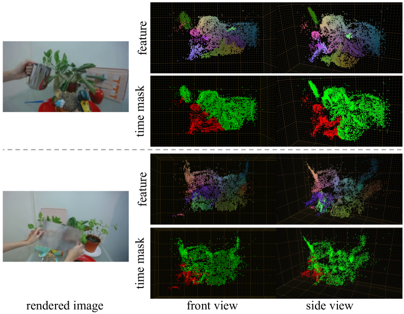
🔼 Figure 6 visualizes the learned anchor features and the predicted time masks. The visualization employs the UMAP technique to reduce the dimensionality of anchor features for easier interpretation. Two scenes are shown, each with a side and front view. The time mask, generated by the time-mask MLP (Φmask), distinguishes between static (green) and dynamic (red) scene regions by classifying anchor points as static or dynamic based on their time-varying attributes. This highlights the network’s ability to differentiate between these two regions without explicit supervision.
read the caption
Figure 6: Visualization of anchor features and time mask. We visualize the rendered images, anchor features, and time masks for two deformation scenes. Anchor features are visualized using the UMAP function. In the time-mask visualization, the time masks are predicted by time-mask MLP ΦmasksubscriptΦ𝑚𝑎𝑠𝑘\varPhi_{mask}roman_Φ start_POSTSUBSCRIPT italic_m italic_a italic_s italic_k end_POSTSUBSCRIPT. Green anchors represent static scenes, while red anchors indicate deformation scenes.
More on tables
| Model | PSNR(dB)↑ | MS-SSIM↑ | FPS↑ |
| Nerfies (Park et al. 2021a) | 22.2 | 0.803 | 1 |
| HyperNeRF (Park et al. 2021b) | 22.4 | 0.814 | 1 |
| TiNeuVox-B (Fang et al. 2022) | 24.3 | 0.836 | 1 |
| 3D-GS (Kerbl et al. 2023) | 19.7 | 0.680 | 32 |
| FFDNeRF (Guo et al. 2023) | 24.2 | 0.842 | 0.05 |
| Deformable 3DGS (Yang et al. 2023) | 25.0 | 0.822 | 13 |
| 4DGS (Wu et al. 2023) | 25.2 | 0.845 | 34 |
| SCGS (Huang et al. 2023) | 24.6 | 0.813 | 12 |
| Ours | 25.7 | 0.860 | 117 |
🔼 This table presents a quantitative comparison of different novel view synthesis methods on the HyperNeRF’s VRIG dataset. The metrics used for comparison include Peak Signal-to-Noise Ratio (PSNR), Multi-Scale Structural Similarity (MS-SSIM), and Frames Per Second (FPS). The rendering resolution for all methods was 960x540 pixels. The best, second-best, and third-best performing methods for each metric are highlighted with color-coding for easy identification and comparison.
read the caption
Table 2: Quantitative results on HyperNeRF’s (Park et al. 2021b) vrig dataset. The rendering resolution is set to 960×\times×540. We color each cell as best, second best, and third best.
| scene | As | Bell | Sieve | |||
| PSNR | FPS | PSNR | FPS | PSNR | FPS | |
| w/o anchor-grid init | 24.57 | 27 | 24.31 | 23 | 24.74 | 17 |
| w/o time-mask | 26.02 | 127 | 25.78 | 132 | 26.18 | 122 |
| full model | 26.65 | 152 | 26.01 | 147 | 27.12 | 151 |
🔼 This table presents an ablation study evaluating the impact of two key components in the proposed Efficient Dynamic Gaussian Splatting (EDGS) method: the anchor-grid initialization strategy and the time-mask Multilayer Perceptron (MLP). The anchor-grid strategy reduces the number of Gaussians needed, which significantly speeds up rendering. The time-mask MLP further enhances speed by identifying and processing only the time-variant (dynamic) anchors, leaving the static anchors unprocessed for better efficiency. The table shows the PSNR (Peak Signal-to-Noise Ratio), a metric for image quality, and the FPS (frames per second), representing the rendering speed, for three scenes under different configurations: using the full model, removing the anchor-grid initialization, and removing the time-mask MLP. The results highlight the contribution of each component to both the speed and quality of the dynamic scene rendering.
read the caption
Table 3: Effects of anchor-voxel strategy and time-mask MLP. The anchor-grid strategy is crucial for rendering speed due to the reduced number of Gaussians. The time-mask MLP filters time-variant anchors, further reducing the number of anchors required for time-variant attribute queries.
| scene | As | Bell | Sieve | |||
| PSNR | SSIM | PSNR | SSIM | PSNR | SSIM | |
| rigid transformation | 23.51 | 0.8259 | 24.21 | 0.8571 | 23.95 | 0.8750 |
| KNN | 25.75 | 0.8954 | 25.53 | 0.8816 | 25.68 | 0.8907 |
| cosine similarity | 26.31 | 0.8928 | 25.74 | 0.8807 | 26.57 | 0.9155 |
| RBF kernel | 26.65 | 0.9015 | 26.01 | 0.9203 | 27.12 | 0.9271 |
🔼 This table compares the performance of four different methods for calculating the changes in Gaussian offset positions over time. The methods are: a rigid transformation approach (assuming all Gaussian offsets move identically to their anchor points); a k-nearest neighbor (KNN) approach; a cosine similarity approach; and a radial basis function (RBF) kernel approach. The table presents the Peak Signal-to-Noise Ratio (PSNR) and Structural Similarity Index (SSIM) for each method across three different scenes from the NeRF-DS dataset, allowing for a comparison of accuracy and quality across varying dynamic scene complexities.
read the caption
Table 4: Gaussian offsets derivation with various strategies. We conduct four different strategies for formulating the variation of the Gaussian offsets across time.
Full paper#
