TL;DR#
Analyzing large datasets with SQL queries can be slow, hindering interactive data exploration. The latency between query submission and result display can frustrate users and limit their ability to discover insights. Current database systems struggle to provide near-instantaneous results for complex, ad-hoc queries due to the time required for planning, compiling, and executing queries on massive datasets. It proposes speculative ad-hoc querying, a novel approach that uses LLMs to speed up the process.
It introduces SpeQL, a system that leverages LLMs to predict likely queries based on the database schema, user history, and incomplete input. Instead of perfect predictions, SpeQL speculates on partial queries, precomputes temporary tables, and continuously displays results for speculated queries. SpeQL exploits precomputation in both query planning and execution, significantly reducing latency. A utility/user study shows SpeQL improves task completion time and helps users discover patterns more quickly.
Key Takeaways#
Why does it matter?#
This paper introduces a new speculative ad-hoc querying paradigm that leverages LLMs to begin query execution before the user finishes typing, significantly reducing query latency and opening new research avenues in interactive data exploration. By integrating LLM-driven speculation with database processing, this work provides a foundation for developing more responsive and user-friendly data analysis tools, which can have a broad impact on research and industry.
Visual Insights#

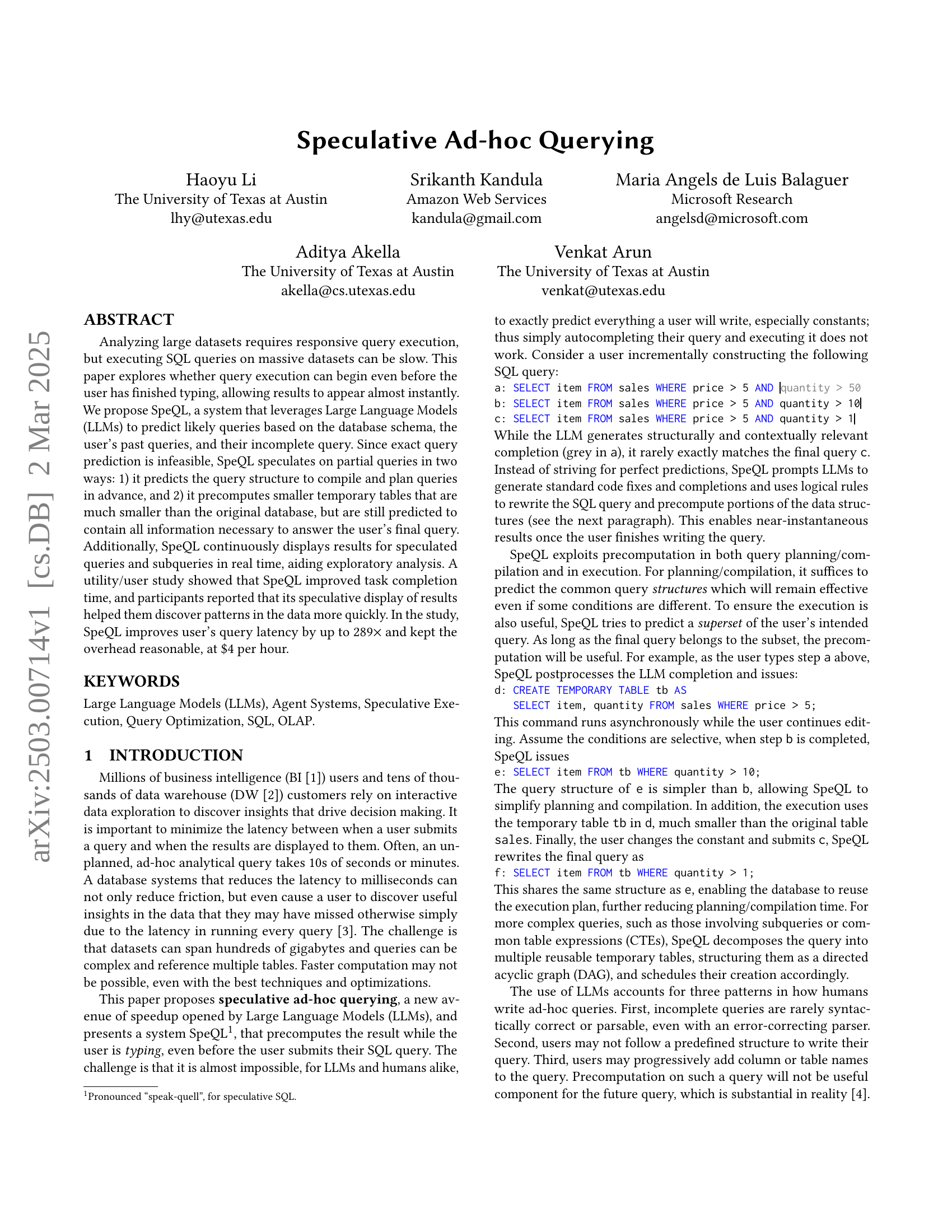
🔼 This figure illustrates SpeQL’s workflow for handling user-edited queries. Each node in the directed acyclic graph (DAG) represents a SELECT statement within the query. SpeQL precompiles and plans these queries, creating temporary tables where possible to optimize execution time. Colored nodes highlight those subqueries that have been precomputed. The system dynamically displays results to the user for the currently highlighted (cursor-selected) part of the query, providing near-instantaneous feedback.
read the caption
Figure 1. SpeQL’s workflow as the user edits the query. Each node represents a SELECT statement. SpeQL structures these nodes as a directed acyclic graph (DAG) and schedules their execution. The colored nodes indicate precomputed subqueries, while the result of the user’s highlighted (cursor-placed) query is previewed to the user.
| 10G/100G/1000G | Median | Mean | Max |
|---|---|---|---|
| LOC in queries | 39 | 48.4 | 227 |
| # of temp tables | 8/7/7 | 10.5/10.1/8.4 | 52/52/44 |
| # of previews | 13/13/11 | 13.5/13.0/11.0 | 21/21/21 |
| # of edges | 37/36/30 | 49.6/48.9/39.6 | 285/285/273 |
| Total size (GB) | 2.0/2.8/3.6 | 5.1/7.5/9.6 | 33.0/39.0/75.9 |
🔼 This table presents a statistical summary of the performance characteristics observed during the benchmarking of SpeQL, a system for speculative ad-hoc querying. The metrics considered include the number of lines of code (LOC) in the queries, the number of temporary tables generated, the number of preview queries executed, the number of edges in the directed acyclic graph (DAG) representing query dependencies, and the total size of these temporary tables in gigabytes (GB). Statistics are provided for three different dataset sizes (10GB, 100GB, and 1000GB), showing median, mean, and maximum values for each metric. This data helps to illustrate the scale and complexity of the queries processed, the amount of pre-computation performed, and the resulting resource usage.
read the caption
Table 1. Benchmarking measurement statistics. “LOC” is short for “lines of code”.
In-depth insights#
Speculative SQL#
The concept of “Speculative SQL,” though not explicitly a heading, is central. It suggests pre-emptive query execution based on user input. LLMs predict likely queries. Key is handling incompleteness and imprecision. Instead of aiming for exact predictions, the system speculates on partial queries: predicting query structure for advanced planning and precomputing temporary tables to contain necessary information for final answers. A continuous display of speculated query results aids exploratory analysis. The system displays the result of the query in its UI. This allows users to iteratively refine their queries with immediate insights. This speculative approach aims to significantly reduce perceived latency, enhancing the interactive data exploration experience. The balance between speculation and overhead is a crucial consideration, and the system likely employs cost-reduction mechanisms.
LLM Query Assist#
While the provided paper does not explicitly use the heading “LLM Query Assist,” the core concept revolves around leveraging Large Language Models (LLMs) to aid users in constructing and executing SQL queries more efficiently. The system, SpeQL, embodies this by using LLMs to debug incomplete queries, autocomplete user inputs, and generate superset queries. These functions directly assist users during the query writing process. By predicting potential query structures and precomputing temporary tables, SpeQL anticipates the user’s needs and minimizes latency. This indirect form of ‘LLM Query Assist’ significantly improves the interactive data exploration experience by making query formulation faster and more intuitive. The paper discusses at length the advantages of such system, and mentions the role of the LLM in the overall architecture.
Precompute Tradeoff#
Precomputation in query processing presents a fundamental tradeoff: investing resources upfront to potentially accelerate future queries versus the risk of wasted effort if those precomputed results aren’t needed. The effectiveness hinges on accurately predicting future query patterns. Overly aggressive precomputation consumes resources and creates maintenance overhead. The key is balancing the scope of precomputation with the likelihood of its reuse. This involves intelligent resource allocation and a deep understanding of the workload characteristics, considering factors like query frequency, data volatility, and storage constraints. A well-designed precomputation strategy carefully assesses these factors, making informed decisions about which results to materialize and when to update them, ultimately optimizing the query processing pipeline for overall performance.
No NL to SQL#
The mention of “No NL to SQL” (Natural Language to SQL) highlights the orthogonal yet complementary nature of SpeQL to NL2SQL systems. While NL2SQL aims to translate human language into SQL, SpeQL focuses on optimizing the execution of SQL queries, regardless of their origin. This implies a potential synergistic relationship: an NL2SQL system could generate a SQL query from user input, and SpeQL could then be applied to speculate and optimize that query’s execution. The paper positions SpeQL as a solution to reduce response latency, while NL2SQL addresses the challenge of lowering the barrier to entry for interacting with databases. Addressing limitations of NL2SQL (ambiguity, database complexity) are not a focus of SpeQL, and vice-versa; the two approaches tackle distinct challenges in the data interaction pipeline. It underscores that NL2SQL and SpeQL can operate independently or be combined to create a more powerful and user-friendly data exploration experience. The combination could significantly enhance data accessibility and analysis efficiency.
Iterative Refine#
The concept of iterative refinement, if applied to query construction, holds significant potential. Users rarely formulate perfect queries on the first attempt; instead, they iteratively refine them based on intermediate results and insights. SpeQL’s approach to displaying speculated results during query construction directly supports this iterative process. By visualizing partial results and potential outcomes, SpeQL allows users to assess the impact of their query modifications and adjust their approach accordingly. This interactive feedback loop accelerates the query formulation process. The LLM plays a crucial role in this by suggesting code fixes and completions, guiding the user towards a syntactically and semantically valid query. However, balancing the usefulness of the LLM suggestions with potential distractions is important to consider. There is an opportunity to refine the LLM prompts and UX to ensure that the suggestions are contextually relevant and actionable, rather than overwhelming the user with irrelevant information This can be implemented with progressive disclosure by showing the most relevant results first, or by allowing the user to customize the type of results displayed.
More visual insights#
More on figures

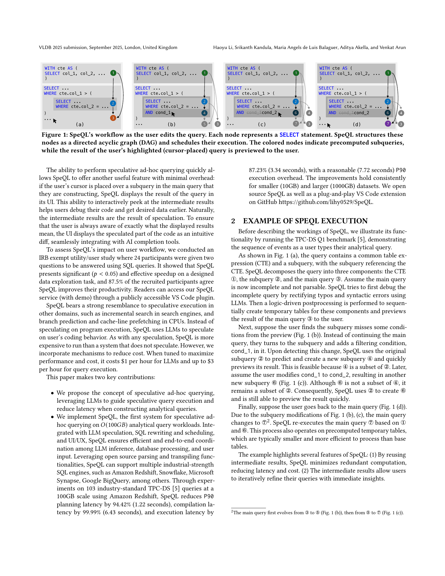
🔼 SpeQL uses a multi-level optimization strategy to handle varying degrees of prediction accuracy from the LLM. Level 0 represents perfect prediction, where the query is precomputed. Level 1 represents partial prediction, where temporary tables that are likely to be used are precomputed. Level 2 represents a basic prefetch of tables and columns likely to be accessed. The figure illustrates how these levels decrease in performance gains as the prediction accuracy decreases.
read the caption
Figure 2. SpeQL proposes a multi-level optimization hierarchy to mitigate varying degrees of misprediction.

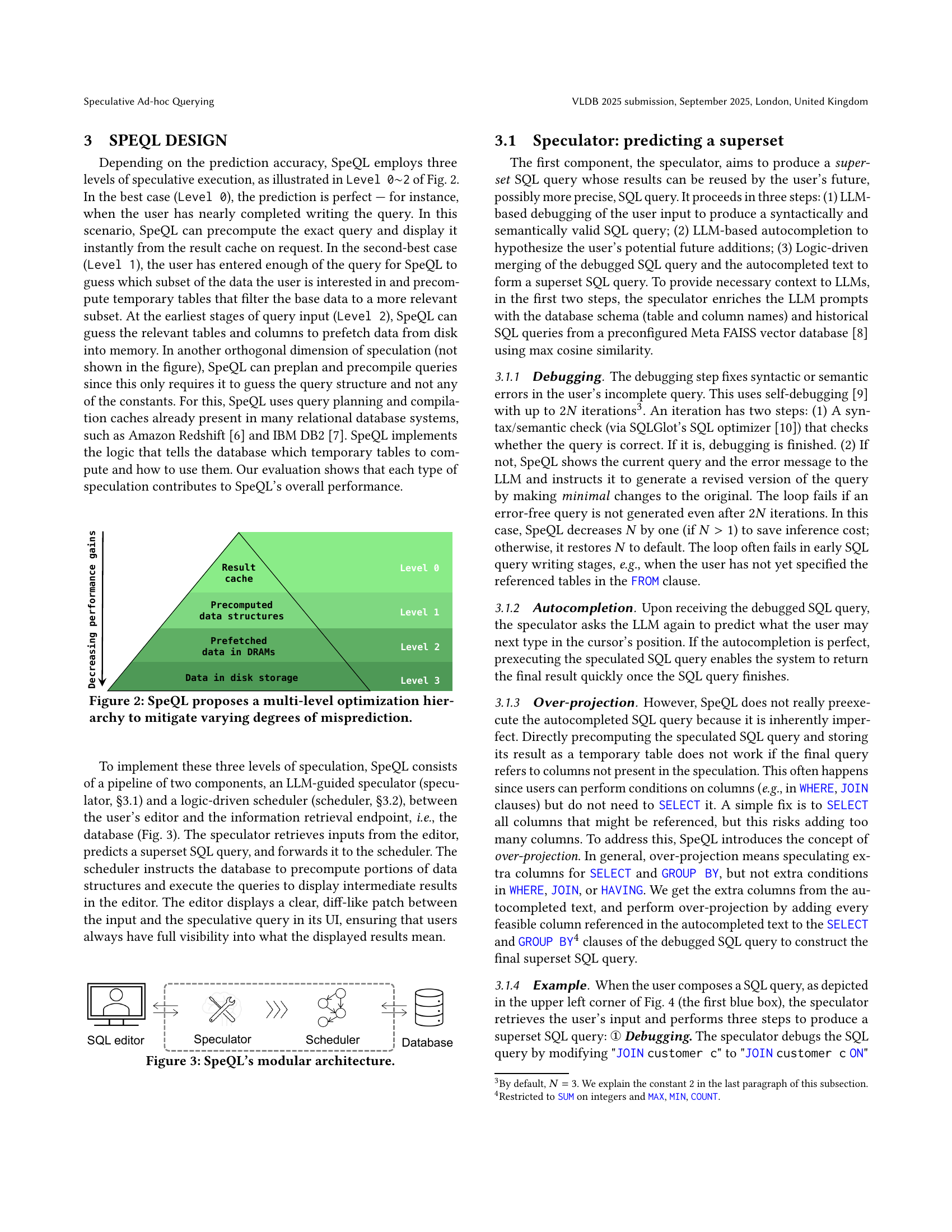
🔼 SpeQL consists of three modules: a speculator, a scheduler, and a database. The speculator receives user input from the SQL editor, uses an LLM to predict the query, and then passes the prediction to the scheduler. The scheduler takes the prediction and sends instructions to the database. The database executes queries and returns results to the editor. The editor displays the results to the user.
read the caption
Figure 3. SpeQL’s modular architecture.

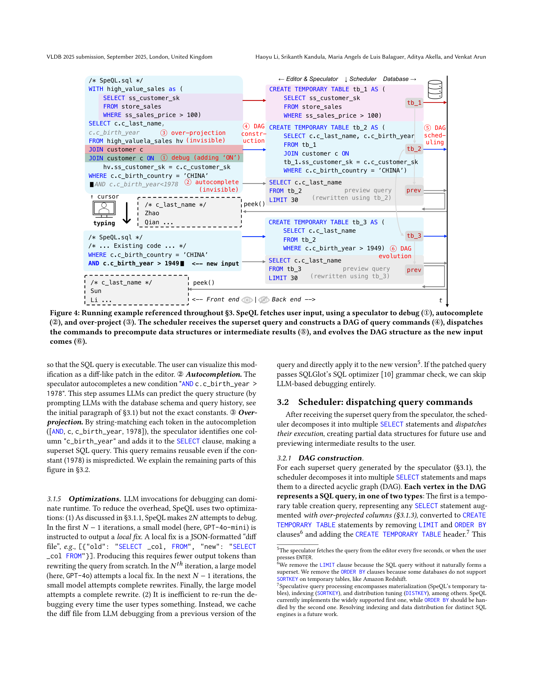
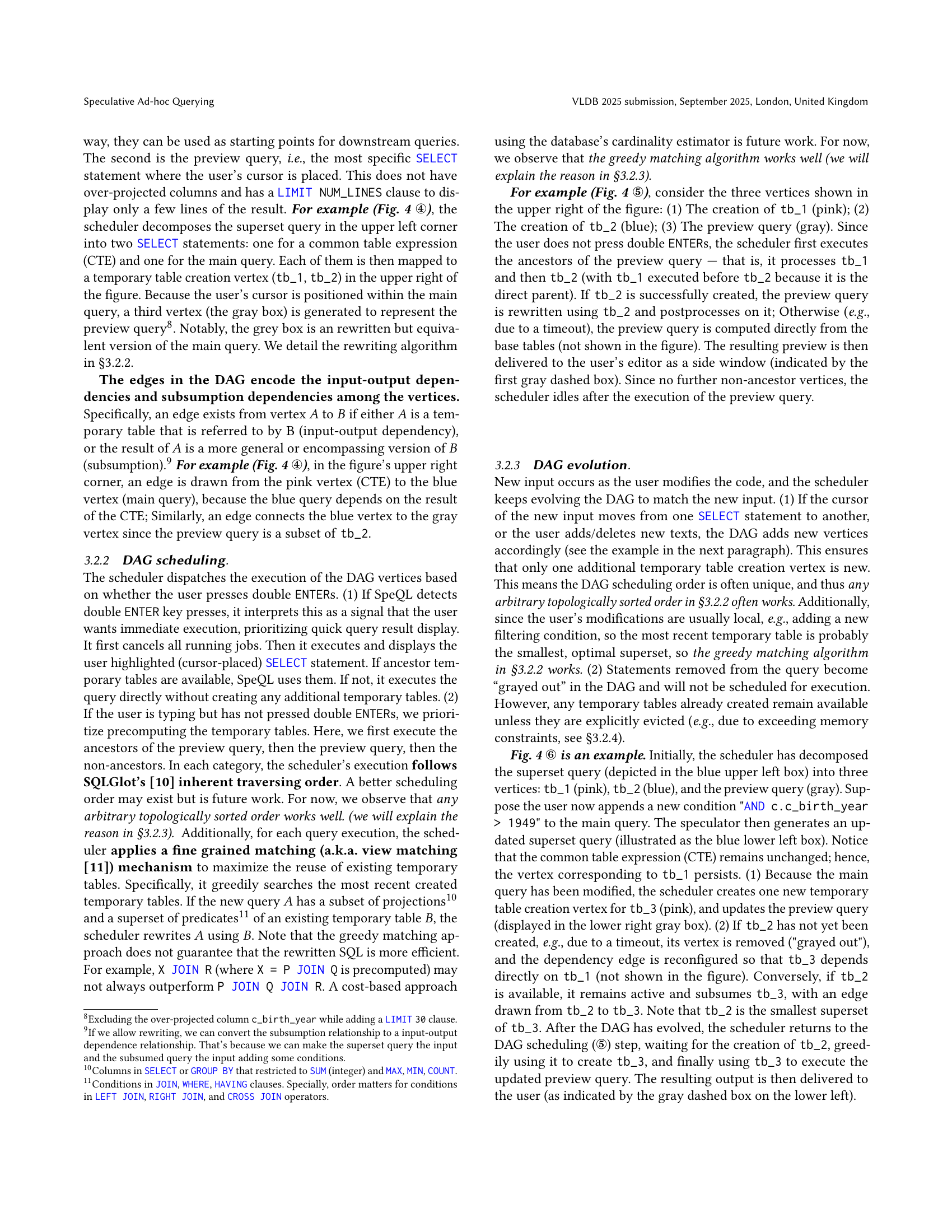
🔼 This figure illustrates the workflow of SpeQL using the TPC-DS Q1 benchmark as an example. It shows how SpeQL processes a user’s incomplete SQL query in six stages: 1) The speculator uses an LLM (Large Language Model) to debug the user’s incomplete SQL query (①), correcting syntax errors and making it semantically valid. 2) The speculator uses the LLM to predict what the user might type next to complete the query (②), providing an autocompletion suggestion. 3) The speculator expands the predicted query to include additional columns to ensure that it will cover the user’s final query. This process is referred to as ‘over-projection’ (③). 4) The scheduler receives the resulting ‘superset’ SQL query and transforms it into a directed acyclic graph (DAG) of smaller, more manageable query commands (④). 5) The scheduler dispatches these commands to the database for precomputation and execution, creating temporary tables and computing partial results (⑤). 6) Finally, as the user continues typing and editing the query, the DAG evolves (⑥) to encompass the new portions of the query. SpeQL continuously previews results from the most recently processed portion of the DAG to the user.
read the caption
Figure 4. Running example referenced throughout §3. SpeQL fetches user input, using a speculator to debug (①), autocomplete (②), and over-project (③). The scheduler receives the superset query and constructs a DAG of query commands (④), dispatches the commands to precompute data structures or intermediate results (⑤), and evolves the DAG structure as the new input comes (⑥).

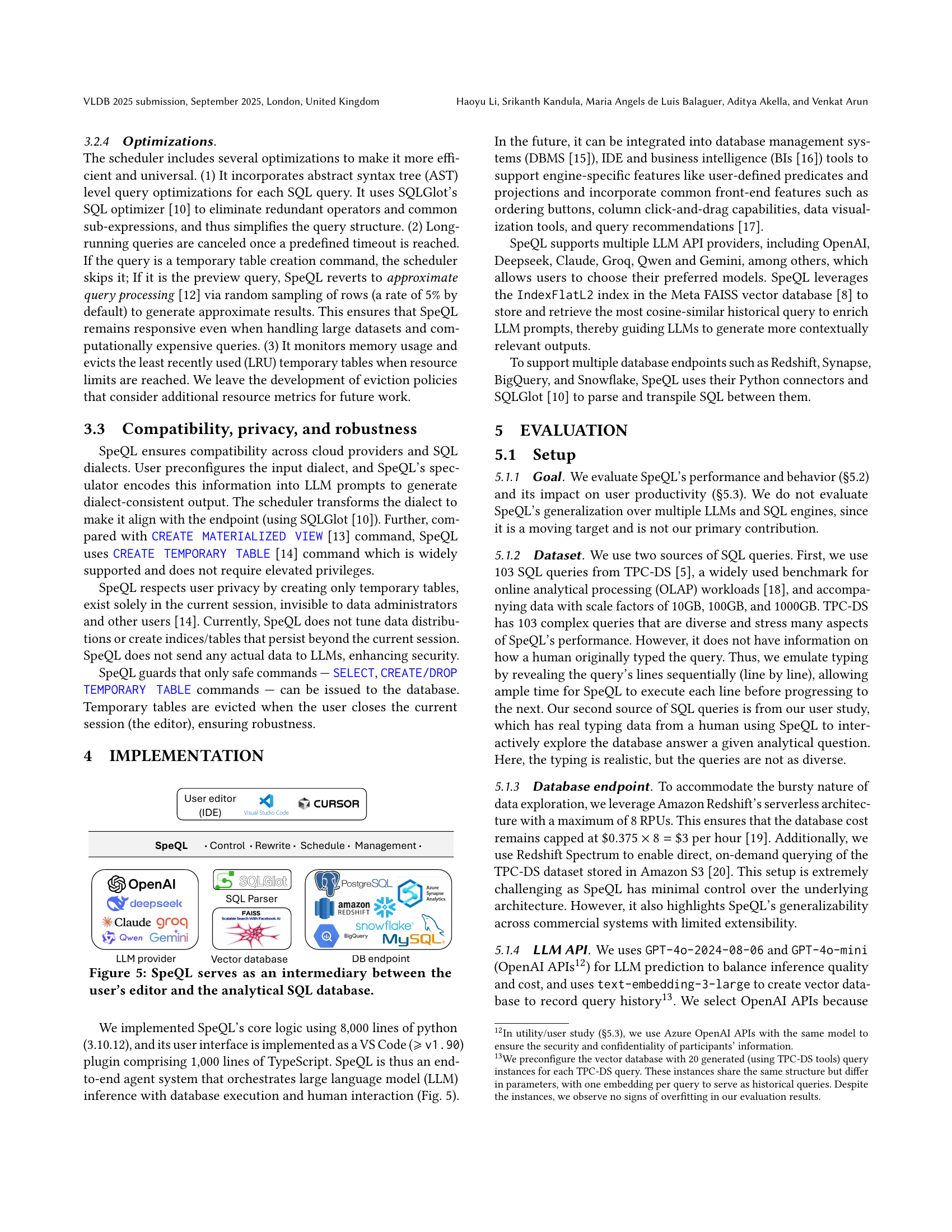
🔼 SpeQL acts as an intermediary between the user’s SQL editor (such as VS Code) and the analytical SQL database. It manages the entire workflow, receiving user input, employing LLMs for prediction and debugging, and orchestrating the interactions between the user’s editor, the LLM(s), the SQL parser (SQLGlot), and the database engine (e.g., Amazon Redshift, Snowflake). The figure visually represents this process flow and highlights the components involved.
read the caption
Figure 5. SpeQL serves as an intermediary between the user’s editor and the analytical SQL database.

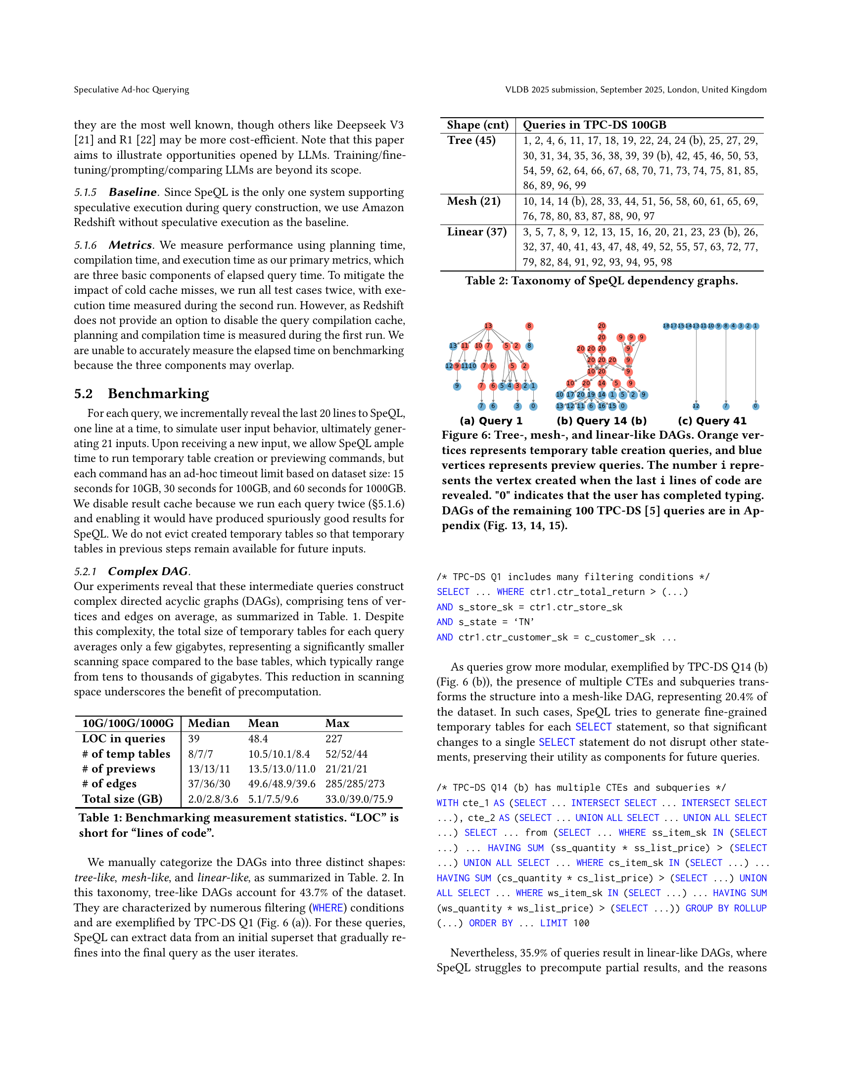
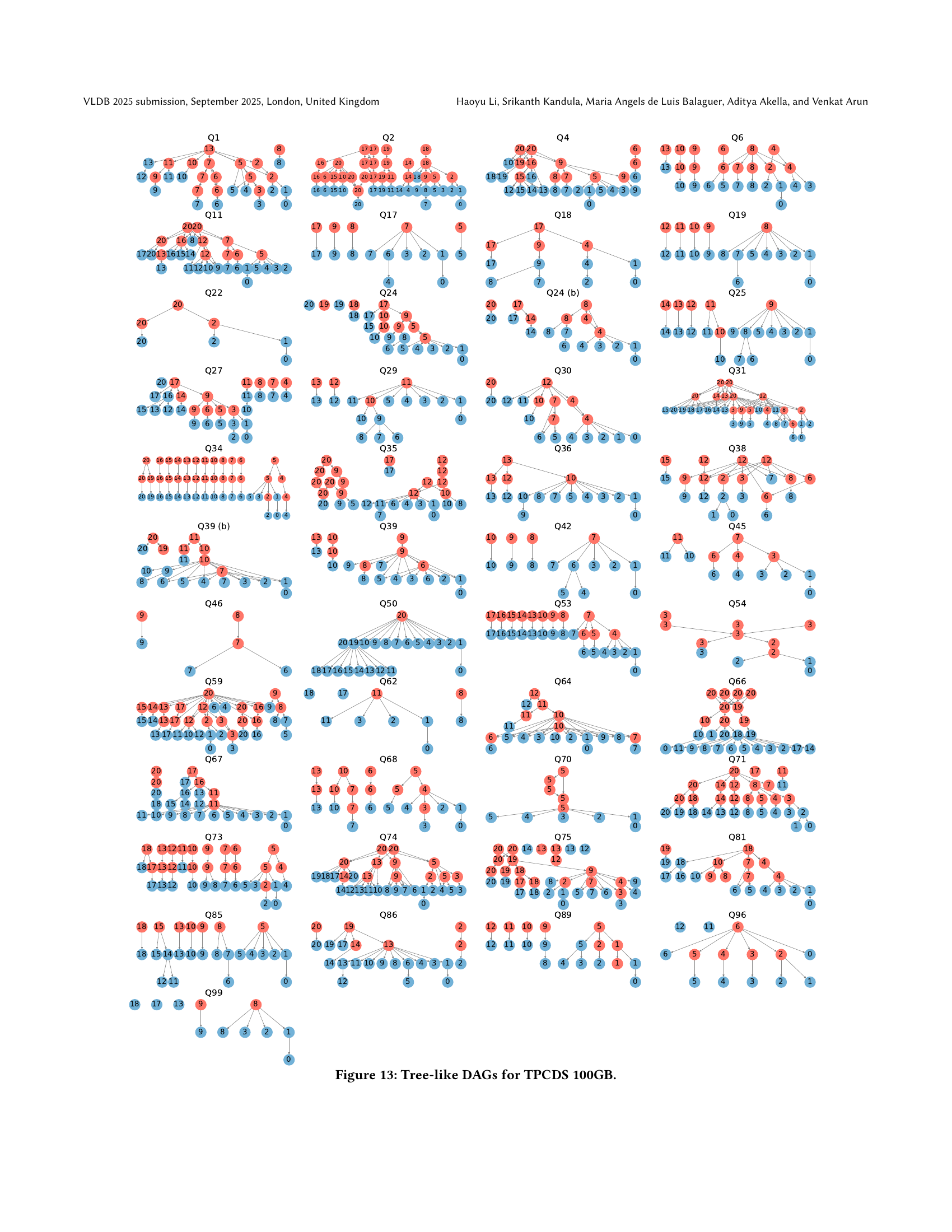
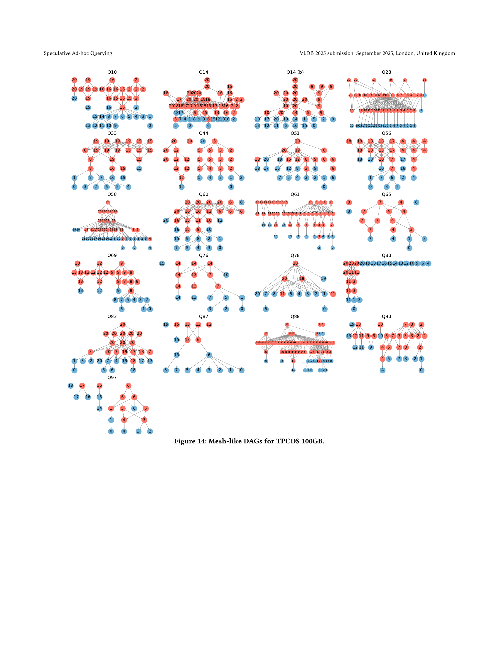
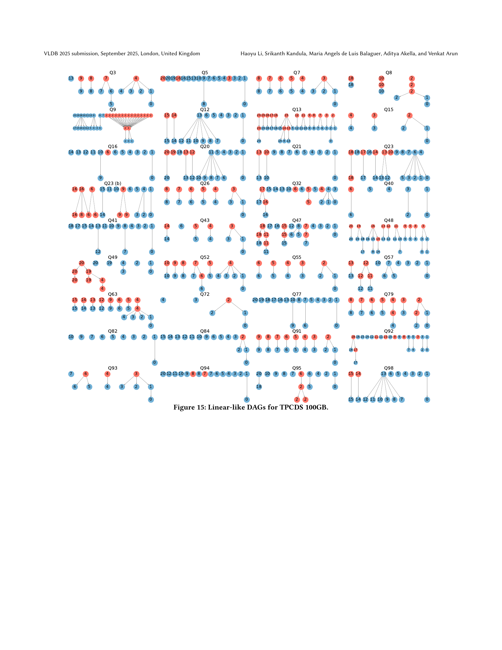
🔼 This figure illustrates the different types of directed acyclic graphs (DAGs) generated by SpeQL during the query construction process, categorized as tree-like, mesh-like, and linear-like. Each node in the DAG represents either a temporary table creation query (orange) or a preview query (blue). The number on each node indicates the order in which it was generated as the user types the query, with ‘0’ representing the final, complete query. The figure shows example DAGs for three TPC-DS queries (Query 1, Query 14(b), and Query 41) with different structures. The DAGs for the remaining 100 TPC-DS queries are shown in the appendix.
read the caption
Figure 6. Tree-, mesh-, and linear-like DAGs. Orange vertices represents temporary table creation queries, and blue vertices represents preview queries. The number i represents the vertex created when the last i lines of code are revealed. ”0” indicates that the user has completed typing. DAGs of the remaining 100 TPC-DS (tpcds, ) queries are in Appendix (Fig. 13, 14, 15).

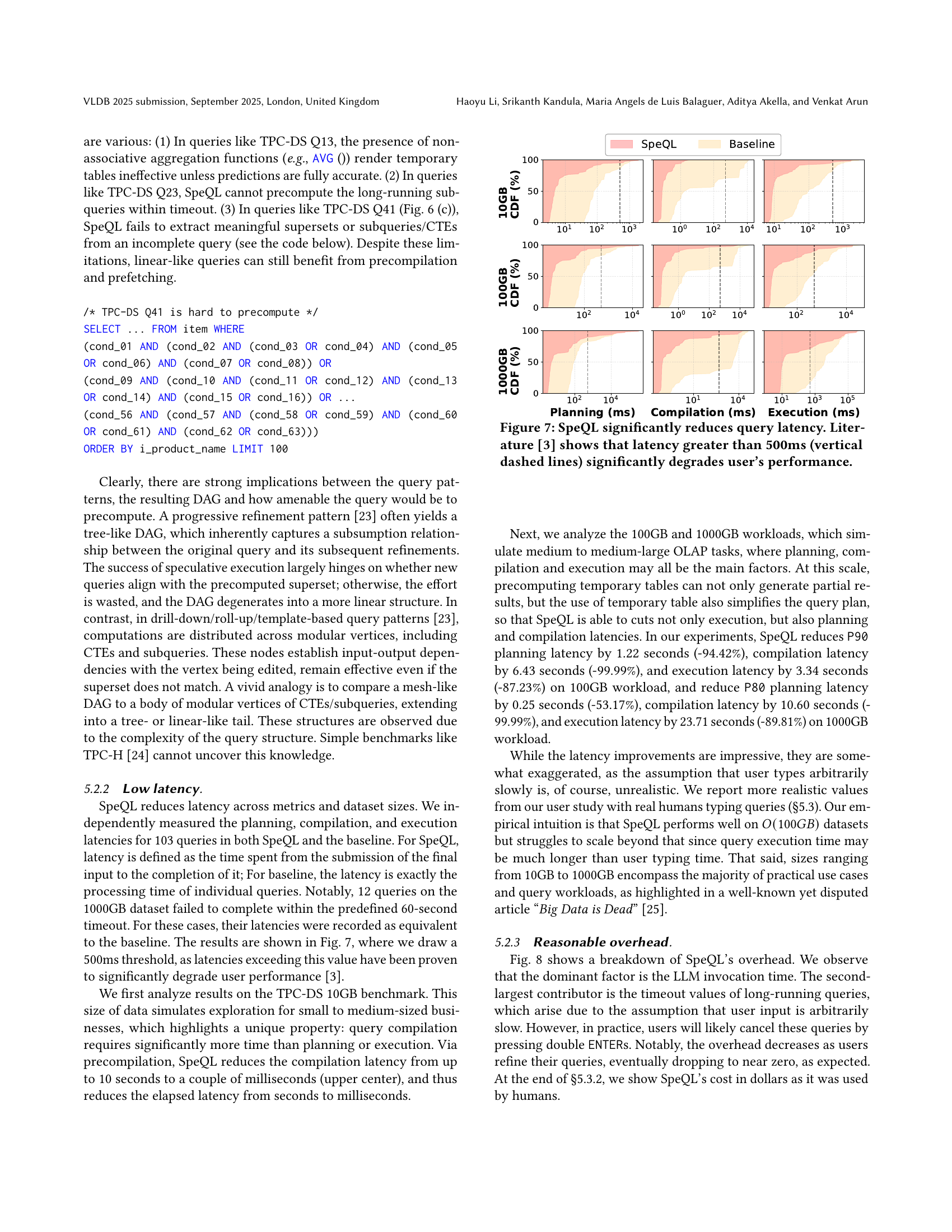
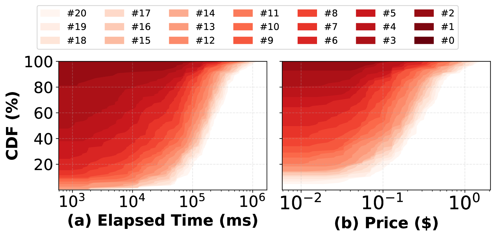
🔼 This figure displays the cumulative distribution function (CDF) plots for query planning, compilation, and execution latency across three different dataset sizes (10GB, 100GB, and 1000GB). The x-axis represents latency in milliseconds (ms) on a logarithmic scale. The y-axis shows the percentage of queries that completed within a given latency. Two sets of curves are shown for each dataset size: one for the baseline system (without speculative execution) and one for SpeQL (with speculative execution). Vertical dashed lines at 500ms highlight the latency threshold identified in prior research as significantly impacting user experience. The plots illustrate SpeQL’s substantial reduction in query latency, especially at higher dataset sizes, and demonstrate that the vast majority of SpeQL queries fall below the 500ms performance threshold, unlike the baseline system which has a significant number of queries that take longer than 500ms.
read the caption
Figure 7. SpeQL significantly reduces query latency. Literature (liu2014effects, ) shows that latency greater than 500ms (vertical dashed lines) significantly degrades user’s performance.

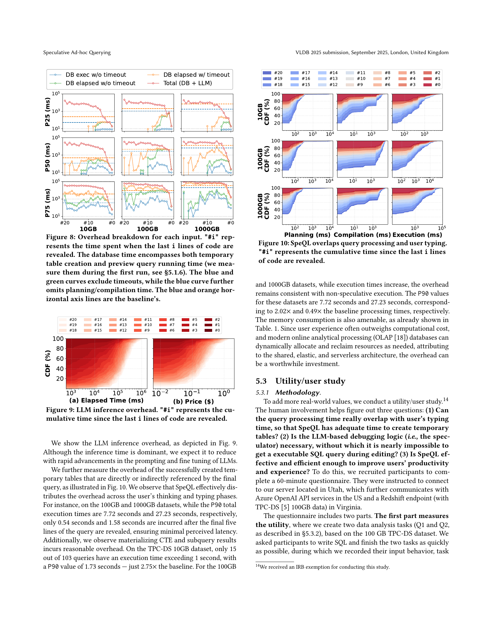
🔼 Figure 8 breaks down the time spent in different parts of SpeQL’s query processing pipeline for TPC-DS queries at various stages of user input (revealed lines of code). It shows the time spent on database operations (including temporary table creation and preview query execution), LLM inference, and total processing time. Different curves illustrate the impact of timeouts on query processing and planning/compilation time. The baseline (no speculation) is also presented for comparison.
read the caption
Figure 8. Overhead breakdown for each input. '#i' represents the time spent when the last i lines of code are revealed. The database time encompasses both temporary table creation and preview query running time (we measure them during the first run, see §5.1.6). The blue and green curves exclude timeouts, while the blue curve further omits planning/compilation time. The blue and orange horizontal axis lines are the baseline’s.
🔼 Figure 9 illustrates the cumulative time spent on LLM inference as more lines of code are added to a SQL query. The x-axis represents the number of lines added, while the y-axis shows the cumulative time. The figure helps to understand how the LLM’s processing time grows as the query becomes more complex and how this relates to the total query time. This is important because it shows a key component of SpeQL’s overhead.
read the caption
Figure 9. LLM inference overhead. '#i' represents the cumulative time since the last i lines of code are revealed.

🔼 Figure 10 illustrates how SpeQL efficiently manages query processing while a user is actively typing. The x-axis represents the cumulative time elapsed since the last ‘i’ lines of code were entered, with ‘#i’ indicating the specific point in time. Different curves represent various percentiles (P25, P50, P75) of latency for different query processing stages: planning, compilation, and execution. The figure visually demonstrates SpeQL’s ability to overlap these processing stages with user input, minimizing the overall query latency.
read the caption
Figure 10. SpeQL overlaps query processing and user typing. '#i' represents the cumulative time since the last i lines of code are revealed.

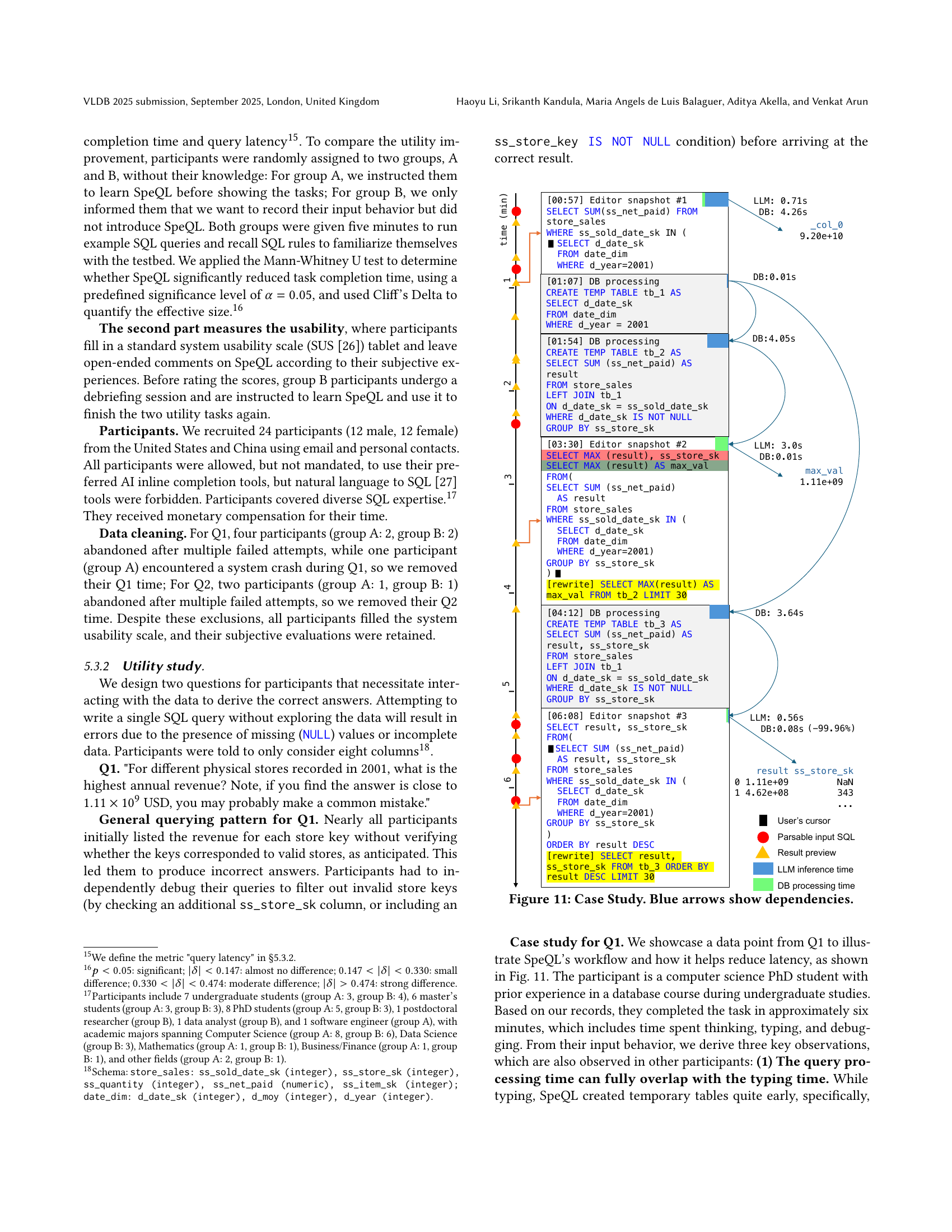
🔼 This figure presents a case study illustrating SpeQL’s workflow. It shows how a user iteratively refines a query, with SpeQL providing intermediate results and debugging assistance. The blue arrows illustrate dependencies between different query components and temporary tables. The timestamps show how the user typed, SpeQL debugged the query, and the database created the temporary tables. The figure demonstrates SpeQL’s ability to overlap query processing time with the user’s typing time, reducing latency significantly.
read the caption
Figure 11. Case Study. Blue arrows show dependencies.
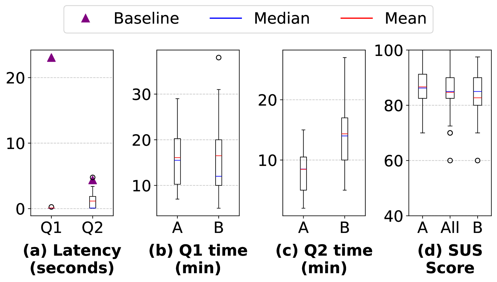
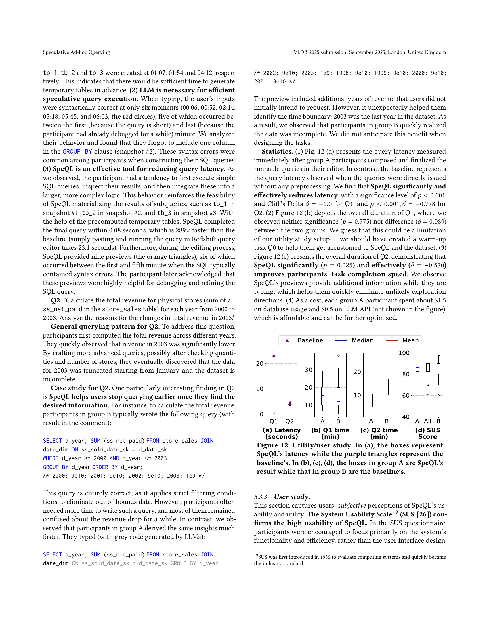
🔼 Figure 12 presents the results of a user study comparing SpeQL’s performance against a baseline system. Panel (a) shows the query latency, comparing SpeQL (boxes) and baseline (purple triangles). The x-axis represents the latency in milliseconds, and the y-axis represents the cumulative distribution function (CDF). Panels (b), (c), and (d) compare the task completion times and usability scores (using SUS) between two groups of participants: group A used SpeQL, and group B used the baseline system. The boxes represent SpeQL’s results and the triangles represent the baseline’s results for each task.
read the caption
Figure 12. Utilily/user study. In (a), the boxes represent SpeQL’s latency while the purple triangles represent the baseline’s. In (b), (c), (d), the boxes in group A are SpeQL’s result while that in group B are the baseline’s.

🔼 This figure visualizes the directed acyclic graphs (DAGs) generated by SpeQL for a subset of the TPC-DS benchmark queries (100GB dataset). Each DAG represents the sequence of temporary table creations and query executions performed by SpeQL as a user progressively constructs a query. The nodes represent individual SQL statements (temporary table creation or a preview query), and the edges depict dependencies between these statements. The color-coding distinguishes between precomputed temporary tables (orange) and preview queries (blue) executed to show intermediate results. The structure of each DAG reflects the complexity of the corresponding query, with varying levels of nested subqueries and CTEs.
read the caption
Figure 13. Tree-like DAGs for TPCDS 100GB.
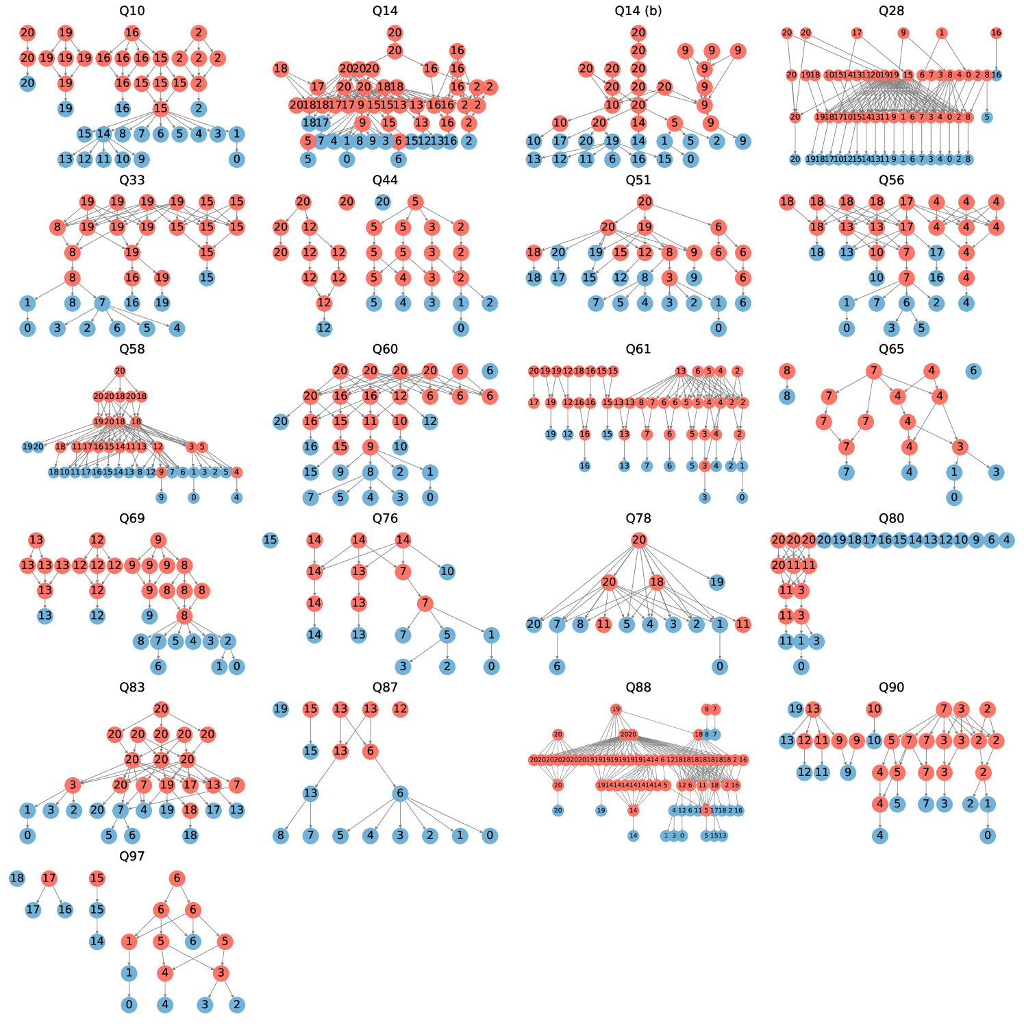
🔼 This figure displays a collection of 21 directed acyclic graphs (DAGs). Each DAG represents the execution plan generated by SpeQL for a specific TPC-DS query in the 100GB dataset. The nodes in the DAGs represent individual SQL queries or temporary table creations, while the edges show dependencies between them. These DAGs illustrate the mesh-like structure resulting from the decomposition of complex queries into smaller, reusable components. The mesh-like structure is characterized by multiple CTEs and subqueries interacting, unlike tree-like DAGs which exhibit a hierarchical structure, or linear-like DAGs which proceed sequentially.
read the caption
Figure 14. Mesh-like DAGs for TPCDS 100GB.

🔼 This figure presents the dependency graphs for queries in the TPC-DS 100GB benchmark dataset that exhibit linear characteristics. Linear-like dependency graphs indicate that the query execution is less amenable to speculative execution compared to tree-like or mesh-like structures. In these linear scenarios, the precomputation of intermediate results and temporary tables is less effective in reducing overall query latency, as there are fewer opportunities to reuse intermediate results for subsequent query refinements.
read the caption
Figure 15. Linear-like DAGs for TPCDS 100GB.
Full paper#