SampleMix: A Sample-wise Pre-training Data Mixing Strategey by Coordinating Data Quality and Diversity

2503.01506

Xiangyu Xi et el.

🤗 2025-03-04

TL;DR
#

Existing data mixing methods for LLMs often determine domain weights and then sample uniformly, neglecting inter-domain overlaps and sample quality. This leads to suboptimal data distribution, hindering effective pre-training due to a failure in controlling global diversity of the constructed training dataset and ignoring fine-grained sample-specific features.

To address these shortcomings, SampleMix employs a bottom-up approach, performing global cross-domain sampling by evaluating the quality and diversity of each sample. It dynamically determines the optimal domain distribution, surpassing existing methods and cutting training steps by 1.4x to 2.1x. SampleMix coordinates quality and diversity, capturing commonalities and optimizing sample distribution.

Key Takeaways
#

Why does it matter?
#

SampleMix offers a novel approach to pre-training data mixing by considering both quality and diversity, leading to more efficient and effective language models. It inspires future research in automatic data evaluation metrics and code data mixing.

Visual Insights
#

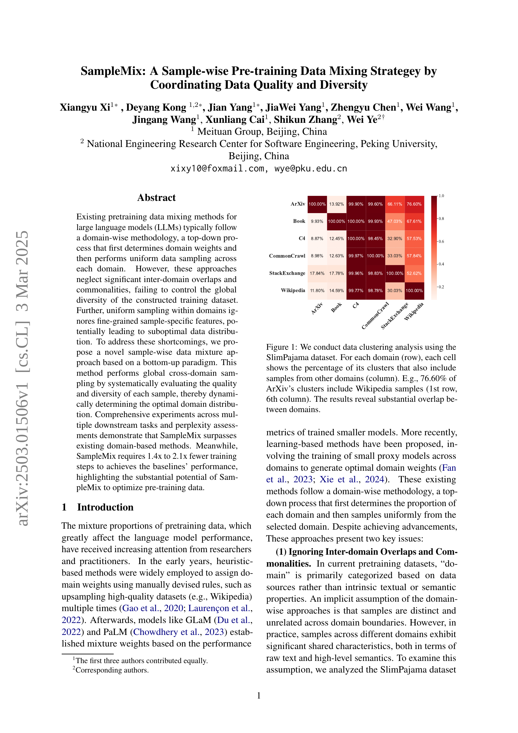
🔼 This figure displays the results of a data clustering analysis performed on the SlimPajama dataset. The analysis reveals the extent of overlap between different domains within the dataset. Each row represents a domain, and each cell within a row shows the percentage of clusters from that domain that also contain samples from another domain (specified by the column). For example, the value in the first row and sixth column indicates that 76.60% of the clusters originating from the ArXiv domain also include samples from the Wikipedia domain. The overall pattern in the figure highlights substantial overlap and interconnectedness between various domains within the SlimPajama dataset, contradicting the common assumption of distinct domain boundaries in pre-training data.
read the caption
Figure 1: We conduct data clustering analysis using the SlimPajama dataset. For each domain (row), each cell shows the percentage of its clusters that also include samples from other domains (column). E.g., 76.60% of ArXiv’s clusters include Wikipedia samples (1st row, 6th column). The results reveal substantial overlap between domains.

Dimension	Score
Clarity of Expression and Accuracy	{0,1}
Completeness and Coherence	{0,1}
Structure and Style	{0,1}
Content Accuracy and Credibility	{0,1}
Significance	{0,1}
Knowledge Richness	{0,1,2}
Logicality and Analytical Depth	{0,1,2}

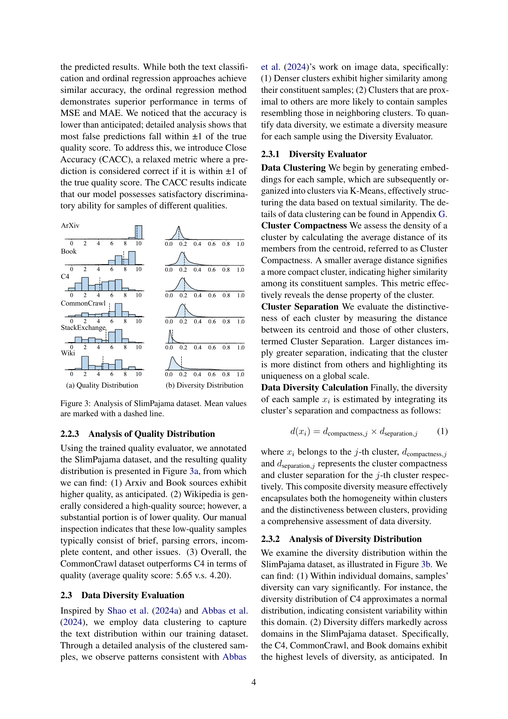
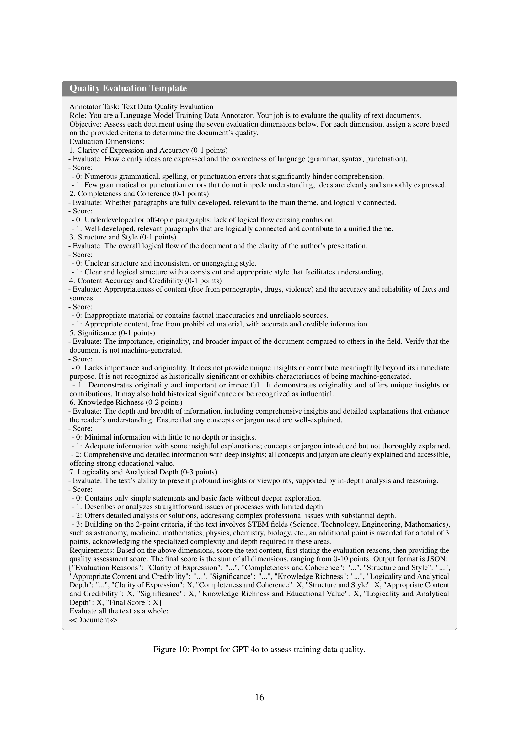
🔼 This table lists the seven dimensions used to evaluate the quality of text data for pre-training language models. Each dimension represents a specific aspect of text quality, such as clarity, completeness, structure, content accuracy, significance, knowledge richness, and logical depth. A numerical score (either 0 or 1, or 0, 1, or 2 depending on the dimension) is assigned to each dimension to reflect the degree to which that aspect is present in the text. The table provides a detailed and comprehensive understanding of the criteria used for data quality assessment.
read the caption
Table 1: Quality dimensions and scores.

In-depth insights
#

Sample-wise Mix
#

Sample-wise mixing seems to be a crucial step in pre-training data construction. Instead of domain-wise strategies, it is more useful to consider the quality and diversity of each sample to determine domain distribution. By assessing each sample, it helps to dynamically determine distribution, allowing more control over dataset quality and diversity. Sampling weights can be assigned based on evaluations, constructing optimal training dataset. It also offers the advantage of dynamically adapting to token budgets, which is useful in the data pre-processing for LLMs.

Quality+Diversity
#

In pre-training data mixing, balancing quality and diversity is crucial for optimal language model performance. High-quality data ensures linguistic precision, structural coherence, and content reliability, while diverse data enhances generalization and prevents overfitting. The interplay between these two factors significantly impacts the model’s ability to capture nuanced patterns and perform well on various downstream tasks. Careful consideration of both aspects is essential when curating pre-training datasets to achieve superior language understanding and generation capabilities. Prioritizing both aspects leads to better model performance and efficiency.

SlimPajama Analysis
#

The paper presents an analysis of the SlimPajama dataset, a cleaned and deduplicated version of RedPajama. The analysis seems to focus on understanding data quality and diversity across different domains within the dataset. This is crucial for pre-training language models, as the composition of the training data significantly impacts model performance. The authors use techniques like data clustering and quality evaluation to gain insights into the characteristics of SlimPajama. They analyze the percentage of cluster that includes other domains to reveal the overlapping of data in SlimPajama. This exploration informs the development of a sample-wise pre-training data mixing strategy, where the quality and diversity of each sample are considered to optimize the training data distribution. By addressing the limitations of domain-wise approaches that often overlook inter-domain commonalities and suboptimal sample distributions, the SlimPajama analysis contributes to creating more effective pre-training datasets for LLMs.

Budget Adaptation
#

Adapting to varying token budgets is a critical capability. Training often involves stages needing different data volumes. Methods with fixed data proportions struggle here. The analysis shows SampleMix’s ability to adjust effectively. When the token budget is small, it smartly discards low-value data. For larger budgets, it prioritizes high-weight samples, highlighting its versatility in resource allocation and effective data selection by ensuring the highest quality data is used first.

Data eval details
#

In analyzing data evaluation details, the focus is on assessing the quality and diversity of datasets used for pre-training large language models. Traditional methods often rely on heuristics, but more sophisticated approaches involve training models to evaluate data quality based on dimensions like linguistic precision, coherence, and content reliability. Diversity is measured using clustering techniques to understand the distribution of text within the dataset. The goal is to create a balanced dataset that enhances the model’s overall performance by prioritizing both quality and diversity. SampleMix is used to determine the optimal balance between these two aspects, adapting to training budgets for effectiveness.

More visual insights
#

More on figures

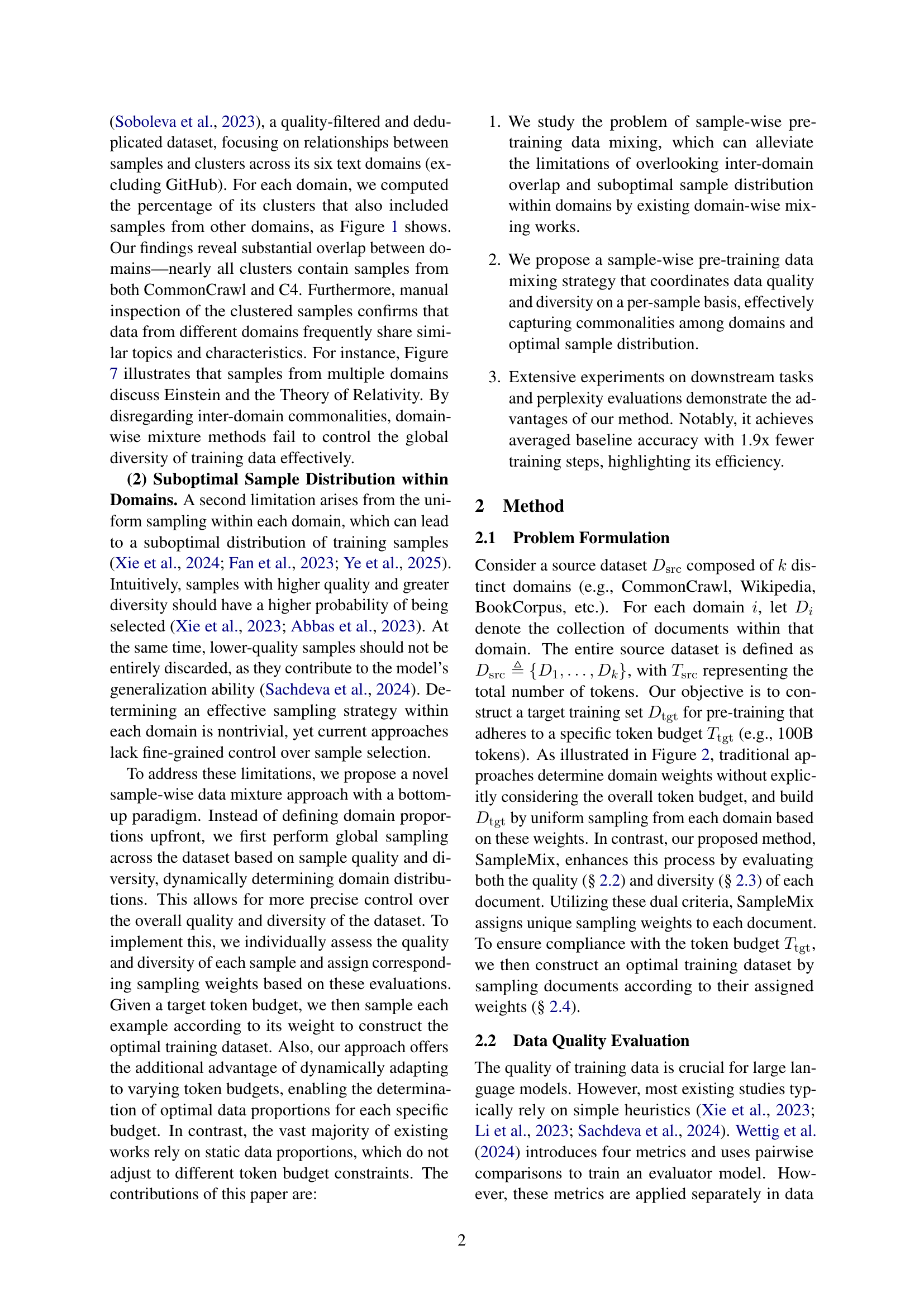
🔼 Figure 2 illustrates the difference between traditional domain-wise data mixing methods and the proposed SampleMix approach. (a) shows the traditional approach where domain weights are determined first and then uniform sampling is performed within each domain. This method ignores the overlap and commonalities among different domains, as well as the sample-specific quality and diversity within each domain. (b) illustrates SampleMix, a novel sample-wise approach. This method dynamically determines domain distributions by systematically evaluating the quality and diversity of each sample. It assigns appropriate weights based on these evaluations and then constructs an optimal training dataset by sampling each example according to its weight. The colors of dots represent different domains, which highlights that this approach considers data from all domains at the same time.
read the caption
Figure 2: (a) Traditional methods determine domain weights and construct the training dataset by uniformly sampling from each domain. (b) SampleMix employs a sample-wise mixing strategy by: evaluating sample quality and diversity, assigning appropriate weights, and constructing an optimal dataset based on these weights. Dots of the same color represent data from the same domain..

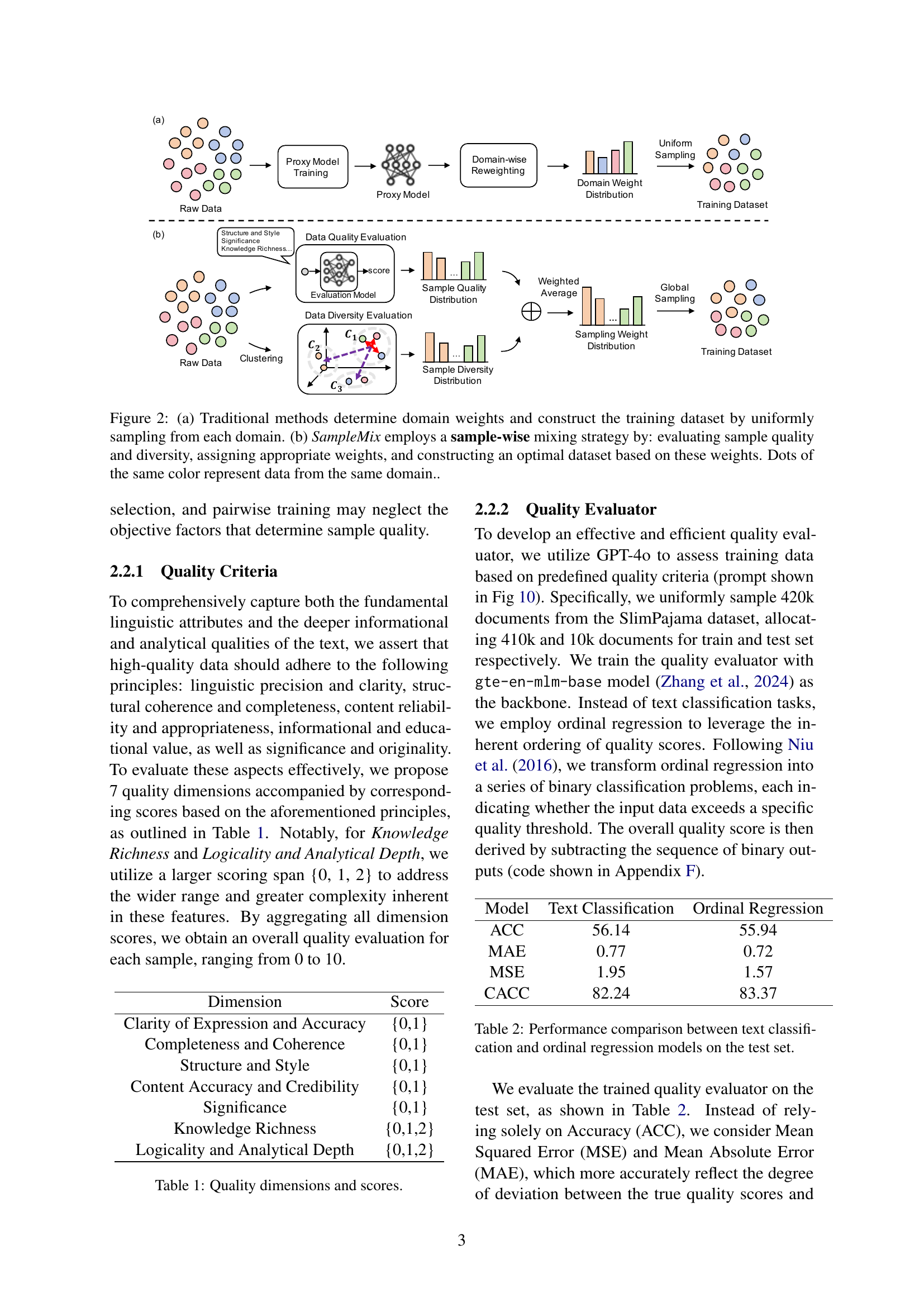
🔼 The figure shows the distribution of quality scores for each of the six domains in the SlimPajama dataset. Each domain’s distribution is shown as a histogram. The x-axis represents the quality score (ranging from 0 to 10), and the y-axis represents the number of samples. The distributions illustrate the varying levels of quality present within each domain. For example, some domains show a higher concentration of high-quality samples (scores closer to 10) while others exhibit a broader spread of quality scores, indicating a greater diversity in data quality.
read the caption
(a) Quality Distribution

🔼 This figure shows the distribution of diversity scores for samples within each domain of the SlimPajama dataset. Each domain’s diversity is assessed using a combined measure of cluster compactness and cluster separation, reflecting how similar samples are within a cluster and how distinct that cluster is from other clusters. The x-axis represents the diversity score, and the y-axis represents the frequency (or percentage) of samples with that diversity score. The figure helps illustrate the variability in diversity within and across different domains of the dataset.
read the caption
(b) Diversity Distribution

🔼 This figure visualizes the distribution of data quality and diversity scores across six domains within the SlimPajama dataset. The left panel (a) shows the distribution of quality scores, revealing variations in the average quality of data across different domains. The right panel (b) displays the distribution of diversity scores, illustrating how diverse the samples are within each domain. Dashed lines indicate the mean values for each distribution.
read the caption
Figure 3: Analysis of SlimPajama dataset. Mean values are marked with a dashed line.

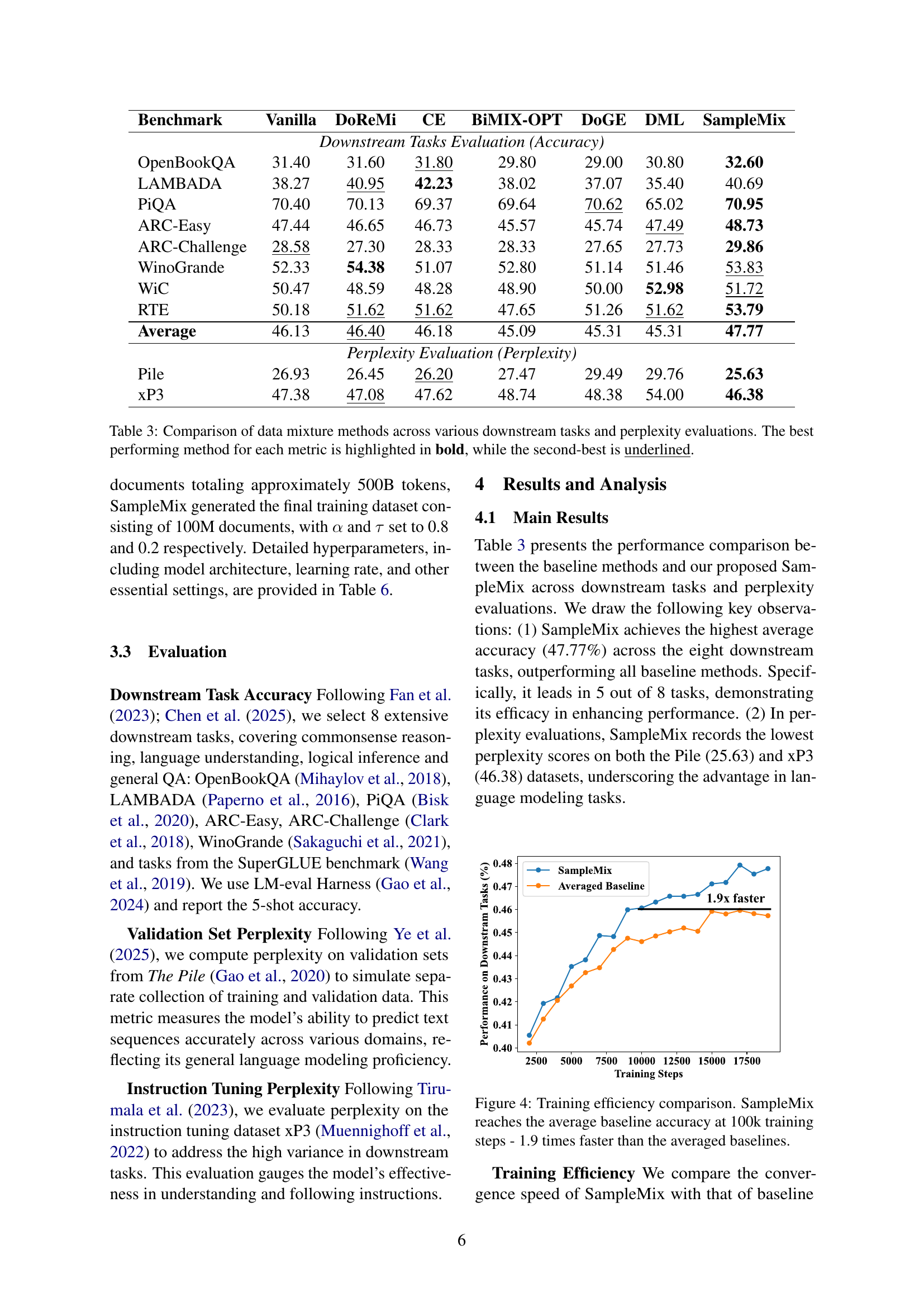
🔼 This figure shows a comparison of the training efficiency between SampleMix and the average performance of several baseline methods. The x-axis represents the number of training steps, and the y-axis represents the accuracy achieved on downstream tasks. The plot shows that SampleMix achieves comparable accuracy to the average baseline performance using significantly fewer training steps – specifically, reaching the average baseline accuracy at approximately 100,000 training steps, which is about 1.9 times faster than the average of the baseline methods.
read the caption
Figure 4: Training efficiency comparison. SampleMix reaches the average baseline accuracy at 100k training steps - 1.9 times faster than the averaged baselines.

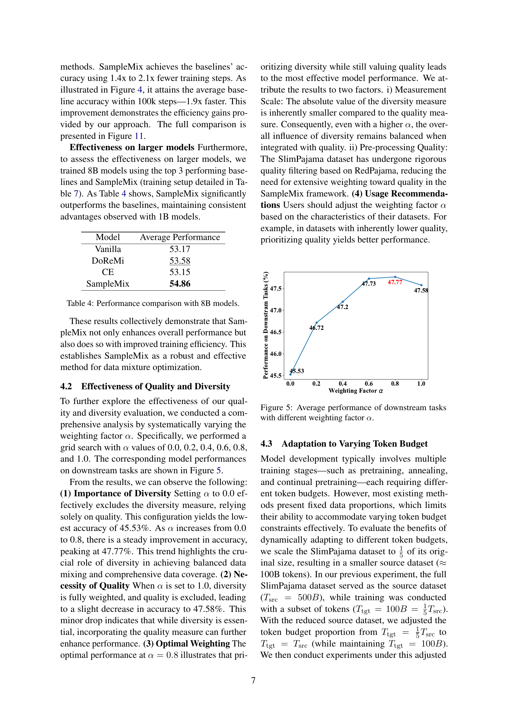
🔼 This figure shows how the weighting factor α (alpha) influences the average performance across various downstream tasks. The x-axis represents different values of α, ranging from 0.0 to 1.0, which controls the balance between quality and diversity in the data sampling process. A value of 0.0 means only quality is considered, while 1.0 means only diversity is considered. The y-axis represents the average performance across all downstream tasks. The plot reveals the optimal balance between quality and diversity that yields the highest average performance, illustrating the impact of different α values on model performance. The figure demonstrates the importance of considering both data quality and diversity for optimal model training.
read the caption
Figure 5: Average performance of downstream tasks with different weighting factor α𝛼\alphaitalic_α.

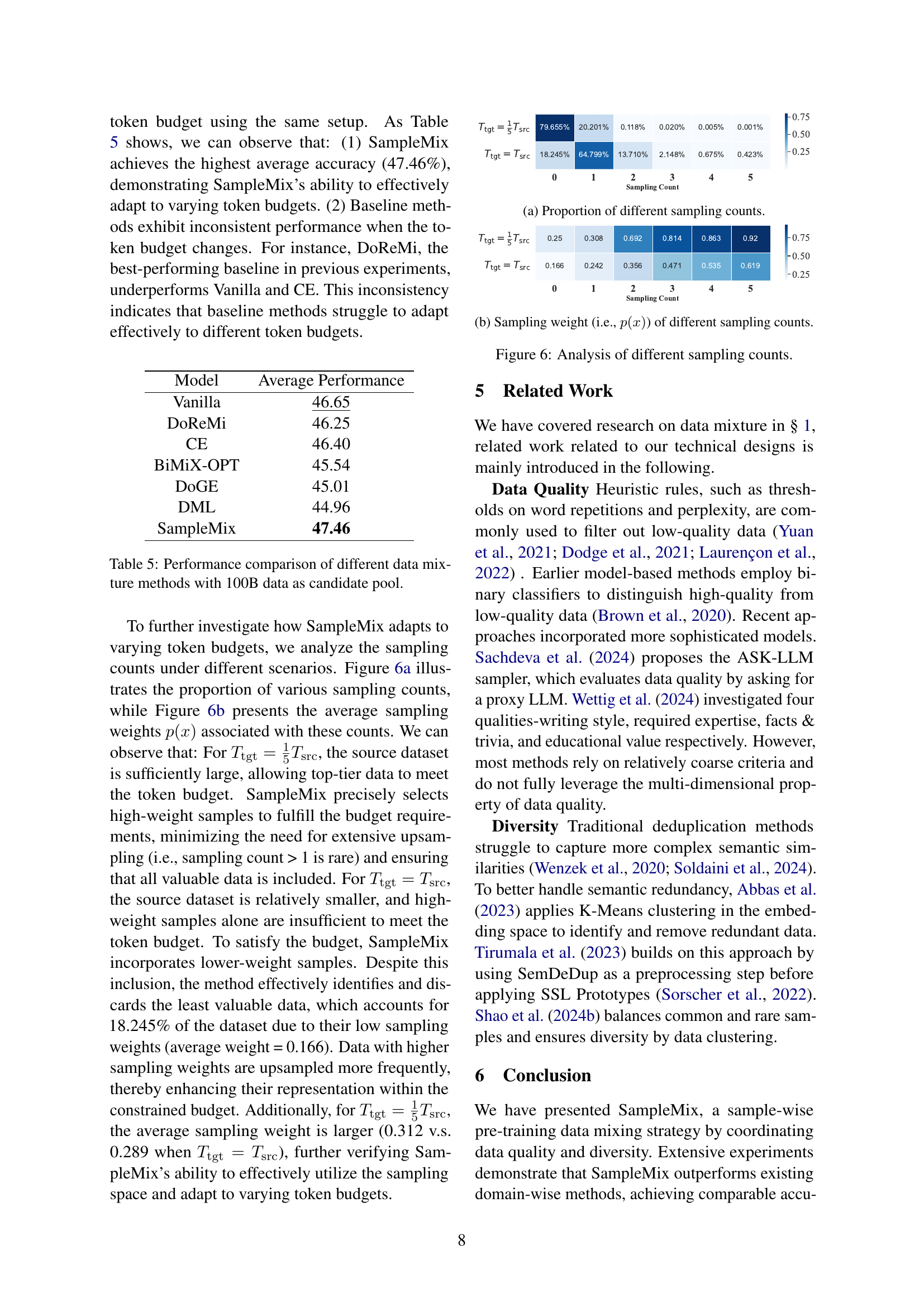
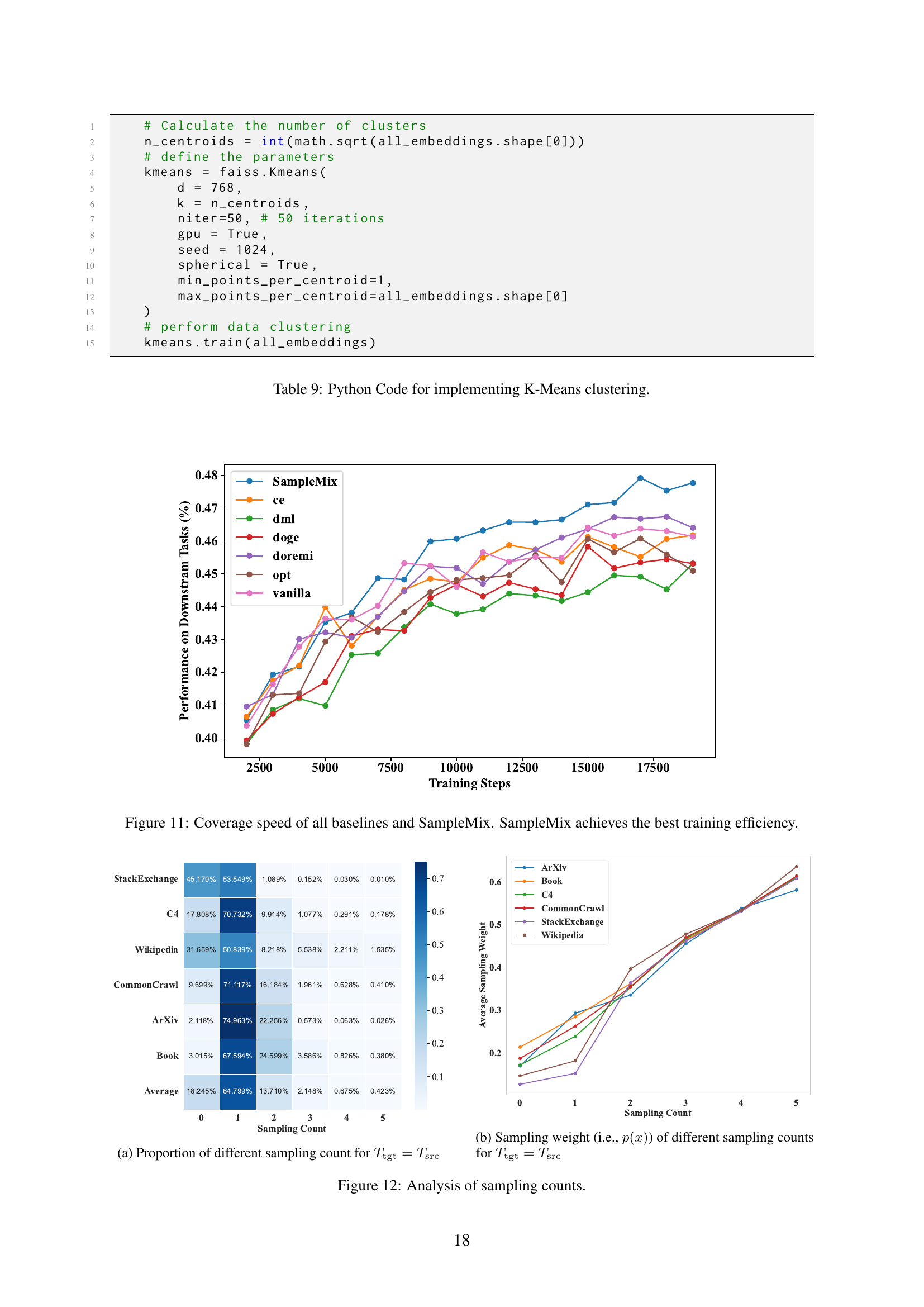
🔼 This figure shows the distribution of the number of times each document was sampled during the training process for the condition where the target token budget (Ttgt) equals the total number of tokens in the source dataset (Tsrc). The x-axis represents the number of times a document was sampled (sampling count), and the y-axis shows the percentage of documents that were sampled that many times. The data illustrates how SampleMix prioritizes high-quality and diverse documents, resulting in many documents being sampled once or twice. A smaller percentage of documents were sampled more frequently, or not at all.
read the caption
(a) Proportion of different sampling counts.

🔼 This figure’s sub-caption describes the relationship between the sampling weight assigned to each data sample and its sampling count, which reflects how many times a particular sample is selected during the training process. In the context of SampleMix, this illustrates how the algorithm prioritizes higher-quality and more diverse samples by assigning them larger sampling weights, leading to increased selection frequency. Conversely, it indicates that lower-quality or less diverse samples may not be chosen as often due to their assigned lower weights. The distribution of weights, therefore, showcases how SampleMix dynamically adjusts to the available data budget, optimizing data diversity, and balancing data quality.
read the caption
(b) Sampling weight (i.e., p⁢(x)𝑝𝑥p(x)italic_p ( italic_x )) of different sampling counts.

🔼 Figure 6 shows the distribution of sampling counts and the corresponding average sampling weights obtained under different token budget settings (Ttgt = Tsrc and Ttgt = Tsrc). When the target token budget (Ttgt) equals the total tokens in the source dataset (Tsrc), SampleMix prioritizes high-quality samples. As a result, the majority of samples are drawn once (sampling count = 1). Conversely, when Ttgt is smaller than Tsrc, the model incorporates samples with lower weights to satisfy the token budget. The figure demonstrates how the model dynamically adapts its sampling strategy based on the available token budget, showcasing SampleMix’s flexibility in handling different training scales.
read the caption
Figure 6: Analysis of different sampling counts.

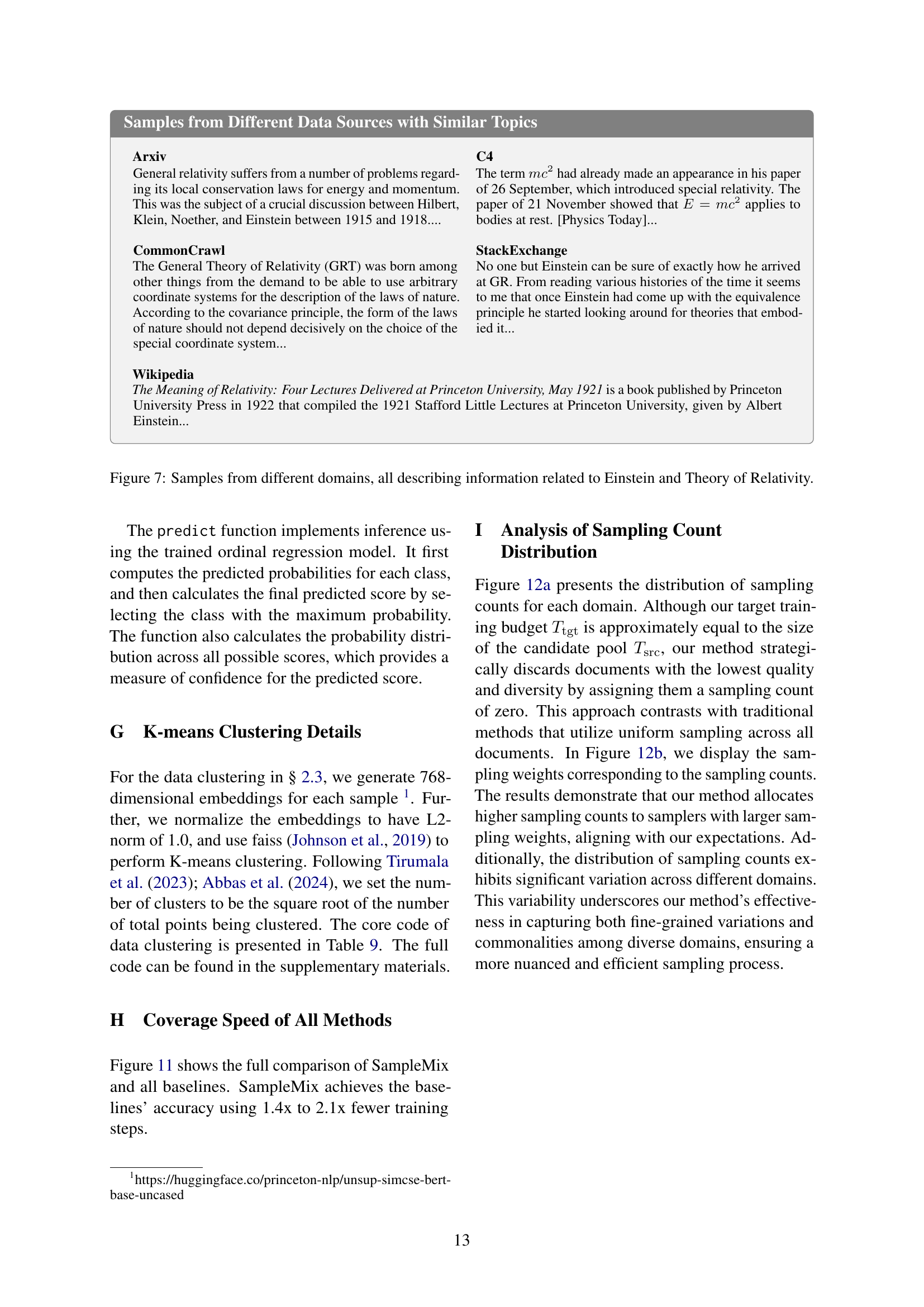
🔼 This figure demonstrates that samples from different datasets, categorized as separate domains, can share significant overlap in terms of topic and semantic content. The examples shown all discuss aspects of Einstein and the Theory of Relativity, highlighting the limitations of domain-wise data mixing approaches that assume strict separation between datasets.
read the caption
Figure 7: Samples from different domains, all describing information related to Einstein and Theory of Relativity.

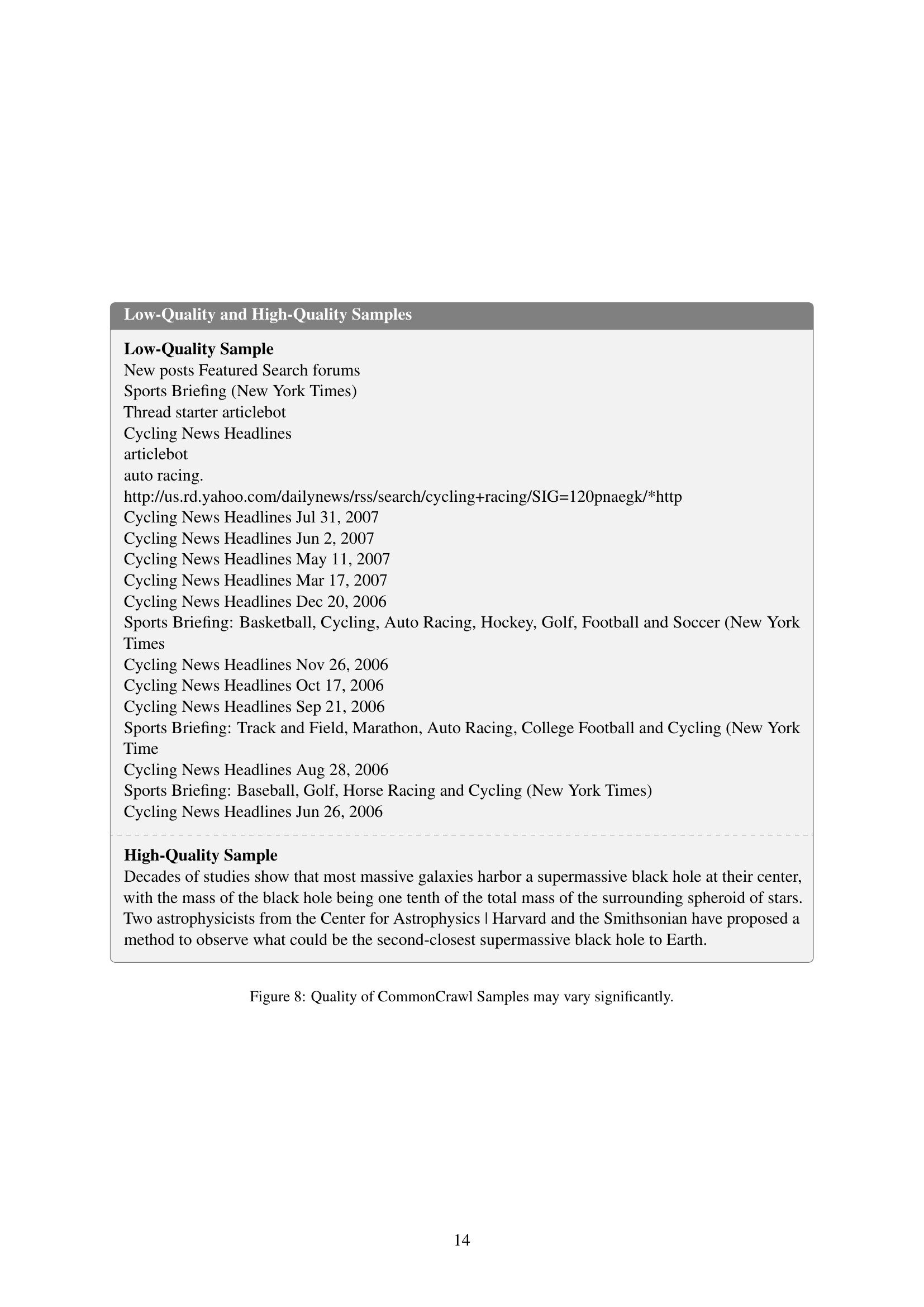
🔼 This figure shows examples of both low-quality and high-quality samples from the Common Crawl dataset. The low-quality example consists of short, seemingly random snippets of text focused on sports news, highlighting the inconsistent and fragmented nature of some data. In contrast, the high-quality example is a coherent, well-structured passage about astrophysics, demonstrating the substantial variation in quality found within the dataset.
read the caption
Figure 8: Quality of CommonCrawl Samples may vary significantly.

More on tables

Model	Text Classification	Ordinal Regression
ACC	56.14	55.94
MAE	0.77	0.72
MSE	1.95	1.57
CACC	82.24	83.37

🔼 This table presents a comparison of the performance of text classification and ordinal regression models in a quality evaluation task. The metrics used to evaluate performance are accuracy (ACC), mean absolute error (MAE), mean squared error (MSE), and close accuracy (CACC). Close accuracy is a relaxed metric where a prediction is considered correct if it’s within ±1 of the true quality score. The results show that while both models achieve similar accuracy, ordinal regression exhibits superior performance in terms of MAE and MSE.
read the caption
Table 2: Performance comparison between text classification and ordinal regression models on the test set.

Downstream Tasks Evaluation (Accuracy)
Benchmark	Vanilla	DoReMi	CE	BiMIX-OPT	DoGE	DML	SampleMix
OpenBookQA	31.40	31.60	31.80	29.80	29.00	30.80	32.60
LAMBADA	38.27	40.95	42.23	38.02	37.07	35.40	40.69
PiQA	70.40	70.13	69.37	69.64	70.62	65.02	70.95
ARC-Easy	47.44	46.65	46.73	45.57	45.74	47.49	48.73
ARC-Challenge	28.58	27.30	28.33	28.33	27.65	27.73	29.86
WinoGrande	52.33	54.38	51.07	52.80	51.14	51.46	53.83
WiC	50.47	48.59	48.28	48.90	50.00	52.98	51.72
RTE	50.18	51.62	51.62	47.65	51.26	51.62	53.79
Average	46.13	46.40	46.18	45.09	45.31	45.31	47.77
Perplexity Evaluation (Perplexity)
Pile	26.93	26.45	26.20	27.47	29.49	29.76	25.63
xP3	47.38	47.08	47.62	48.74	48.38	54.00	46.38

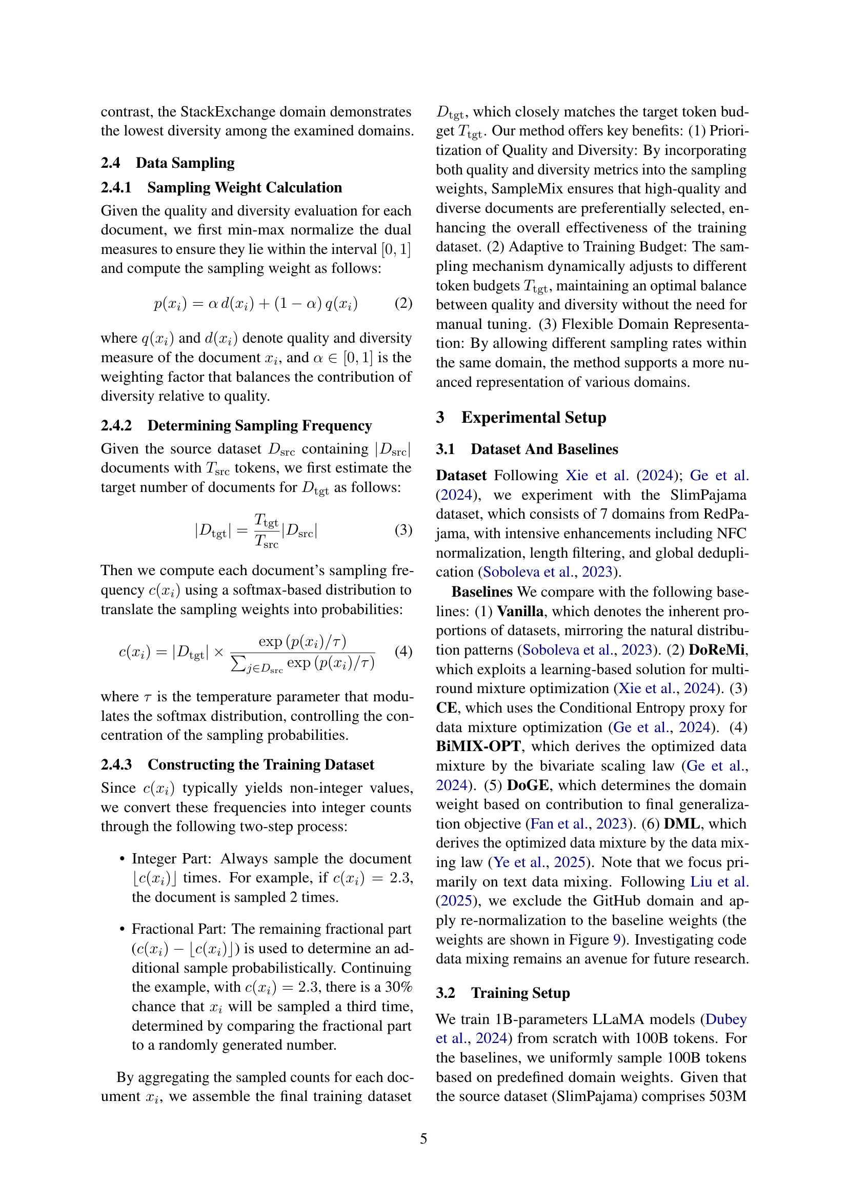
🔼 This table compares the performance of several data mixing methods for large language models across multiple downstream tasks and perplexity evaluations. The methods are compared based on their accuracy on eight different tasks (OpenBookQA, LAMBADA, PIQA, ARC-Easy, ARC-Challenge, WinoGrande, WiC, and RTE) and their perplexity scores on two benchmark datasets (Pile and xP3). The best-performing method for each metric is shown in bold, while the second-best is underlined. This allows for a direct comparison of the different methods’ effectiveness in improving model performance and generalizability across a range of tasks and datasets.
read the caption
Table 3: Comparison of data mixture methods across various downstream tasks and perplexity evaluations. The best performing method for each metric is highlighted in bold, while the second-best is underlined.

Model	Average Performance
Vanilla	53.17
DoReMi	53.58
CE	53.15
SampleMix	54.86

🔼 This table presents a comparison of the average performance achieved by different data mixture methods using 8B parameter models. It shows the average performance across various downstream tasks for each method, allowing for a direct comparison of the effectiveness of different approaches when scaling up the model size.
read the caption
Table 4: Performance comparison with 8B models.

Model	Average Performance
Vanilla	46.65
DoReMi	46.25
CE	46.40
BiMiX-OPT	45.54
DoGE	45.01
DML	44.96
SampleMix	47.46

🔼 This table presents a comparison of different data mixing methods’ performance when the total number of tokens in the training dataset is fixed at 100 billion. It contrasts the performance of various methods under a reduced candidate pool of data. The comparison includes the average performance across multiple downstream tasks, highlighting the effectiveness of the different methods under constrained data conditions.
read the caption
Table 5: Performance comparison of different data mixture methods with 100B data as candidate pool.

Hyper-parameter	Value
layer num	28
attention head num	13
attention head dim	128
model dim	1664
ffn intermediate dim	4480
global batch size	1280
sequence length	4096
learning rate	$2e^{-4}$
learning rate scheduler	cosine scheduler
learning rate warmup tokens	525M

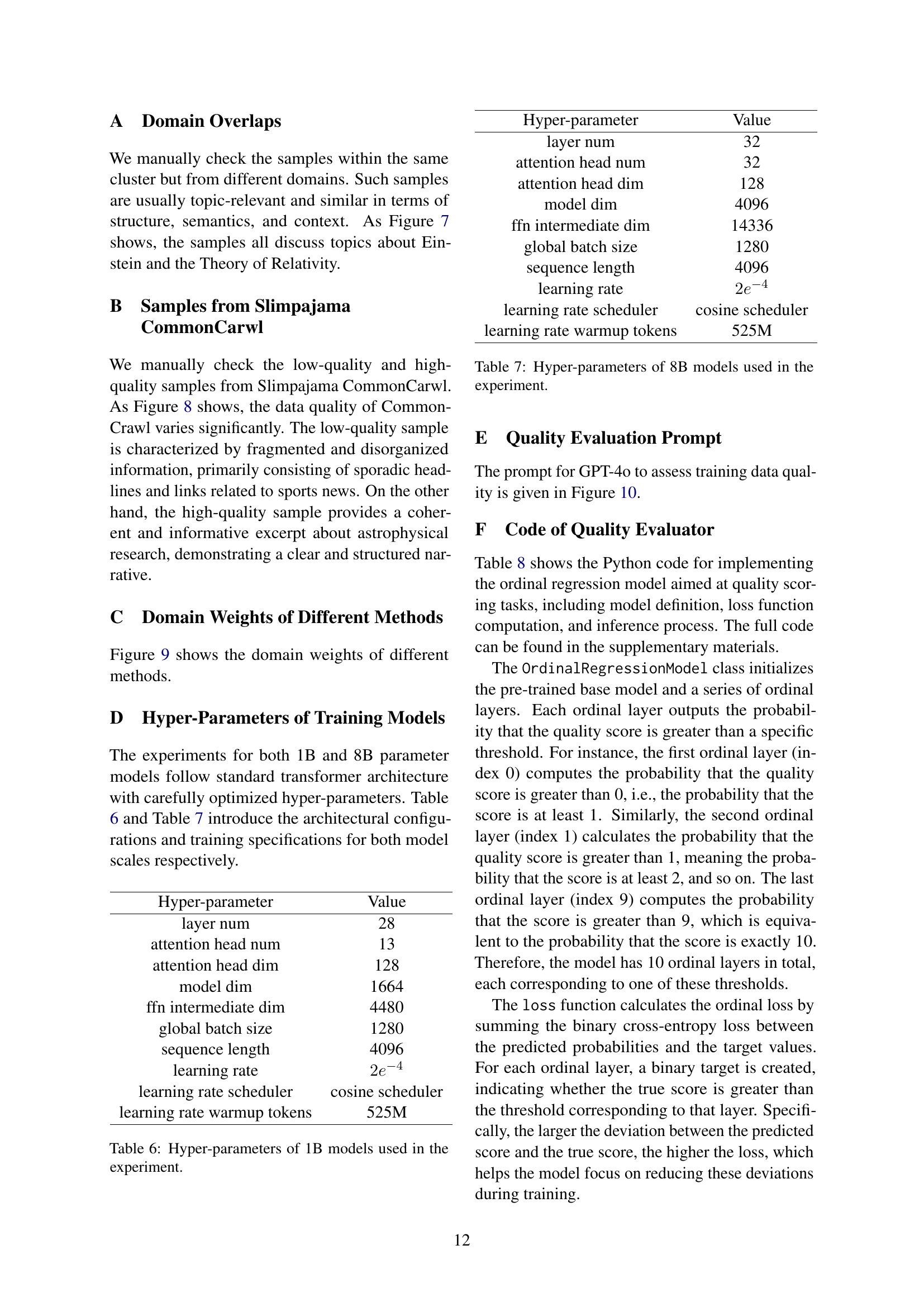
🔼 This table details the hyperparameters used for training the 1-billion parameter Language Model (LLM). These settings encompass various architectural choices and training configurations, influencing the model’s performance and efficiency. The listed hyperparameters include the number of layers, the dimensions of attention heads and the feed-forward network, batch size, sequence length during training, the learning rate and its scheduling scheme (including the number of warmup tokens), all crucial aspects determining the model’s final characteristics.
read the caption
Table 6: Hyper-parameters of 1B models used in the experiment.

Hyper-parameter	Value
layer num	32
attention head num	32
attention head dim	128
model dim	4096
ffn intermediate dim	14336
global batch size	1280
sequence length	4096
learning rate	$2e^{-4}$
learning rate scheduler	cosine scheduler
learning rate warmup tokens	525M

🔼 This table lists the hyperparameters used for training the 8-billion parameter language models in the experiment. It details the architectural configuration, including the number of layers, attention heads, dimensions of various components (attention head, model, feed-forward network), batch size, sequence length, learning rate, learning rate scheduler, and the number of warmup tokens used during training.
read the caption
Table 7: Hyper-parameters of 8B models used in the experiment.

TL;DR#

Key Takeaways#

Why does it matter?#

Visual Insights#

In-depth insights#

Sample-wise Mix#

Quality+Diversity#

SlimPajama Analysis#

Budget Adaptation#

Data eval details#

More visual insights#

Full paper#