TL;DR#
Large reasoning models (LRMs) enhance complex tasks by generating extended thought processes. Unlike one-time train-time scaling, test-time scaling learns to trade more token outputs for improved performance. This requires models to generate and employ critical reasoning steps, enabling solution searches within the natural language space. Current methods use rule-based rewards with verifiable problems, but general applicability remains challenging in complex scenarios.
This research explores scaling reinforcement learning (RL) training for LRMs as part of the STILL project. The study experiments with diverse factors influencing RL training, focusing on base and fine-tuned models. The RL approach improves base models (QWEN2.5-32B) consistently, enhancing response length and test accuracy. Refining models like DEEPSEEK-R1-DISTILL-QWEN-1.5B through RL reaches AIME 2024 accuracy of 39.33%. Tool manipulation further enhances large reasoning models, achieving 86.67% accuracy on AIME 2024 with greedy search.
Key Takeaways#
Why does it matter?#
This research provides valuable insights into training effective reasoning models, paving the way for future advancements in complex AI systems. The exploration of tool manipulation and RL techniques offers new avenues for enhancing model capabilities and solving intricate problems.
Visual Insights#

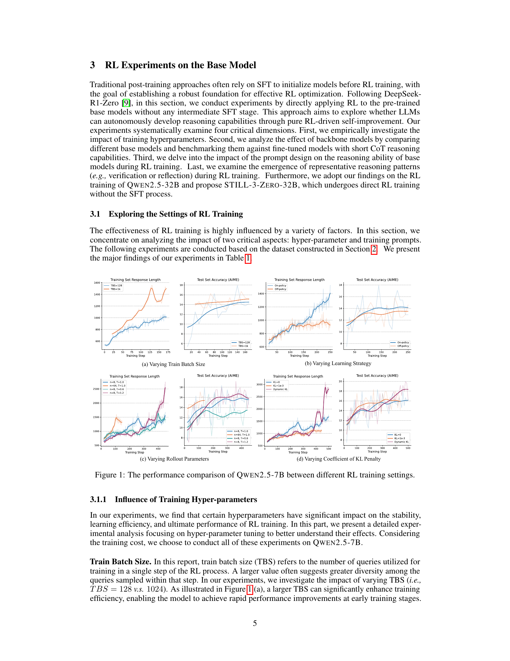
🔼 This figure compares the performance of the QWEN2.5-7B model under various RL training settings. It shows the training set response length and test set accuracy (on AIME) across different hyperparameters, including training batch size, learning strategies (on-policy vs. off-policy), rollout parameters (number of times and temperature), and the coefficient of KL penalty. Each subplot illustrates the impact of varying one hyperparameter while holding others constant, revealing the effects of these parameters on training efficiency and model performance.
read the caption
Figure 1: The performance comparison of Qwen2.5-7B between different RL training settings.
| Factor | Explored Options | Recommended Option |
| Train Batch Size | (Enhancing the training efficiency) | |
| Learning Strategy | On-policy Training | On-policy Training (Enhancing the training efficiency) |
| Off-policy Training | ||
| Rollout Times | (Expanding exploration space) | |
| Rollout Temperature | (Expanding exploration space) | |
| Coefficient of KL | Dynamic KL Annealing (Balancing constraints and exploration) | |
| Dynamic KL Annealing | ||
| Backbone Model | Qwen2.5-1.5B | Qwen2.5-32B (Possessing stronger learning capacities) |
| Qwen2.5-7B | ||
| Qwen2.5-32B | ||
| Qwen2.5-7B-Instruct | ||
| Training Prompt | Simple Instruction | Detailed Instruction (Enhancing reasoning efficiency of the model) |
| Detailed Instruction |
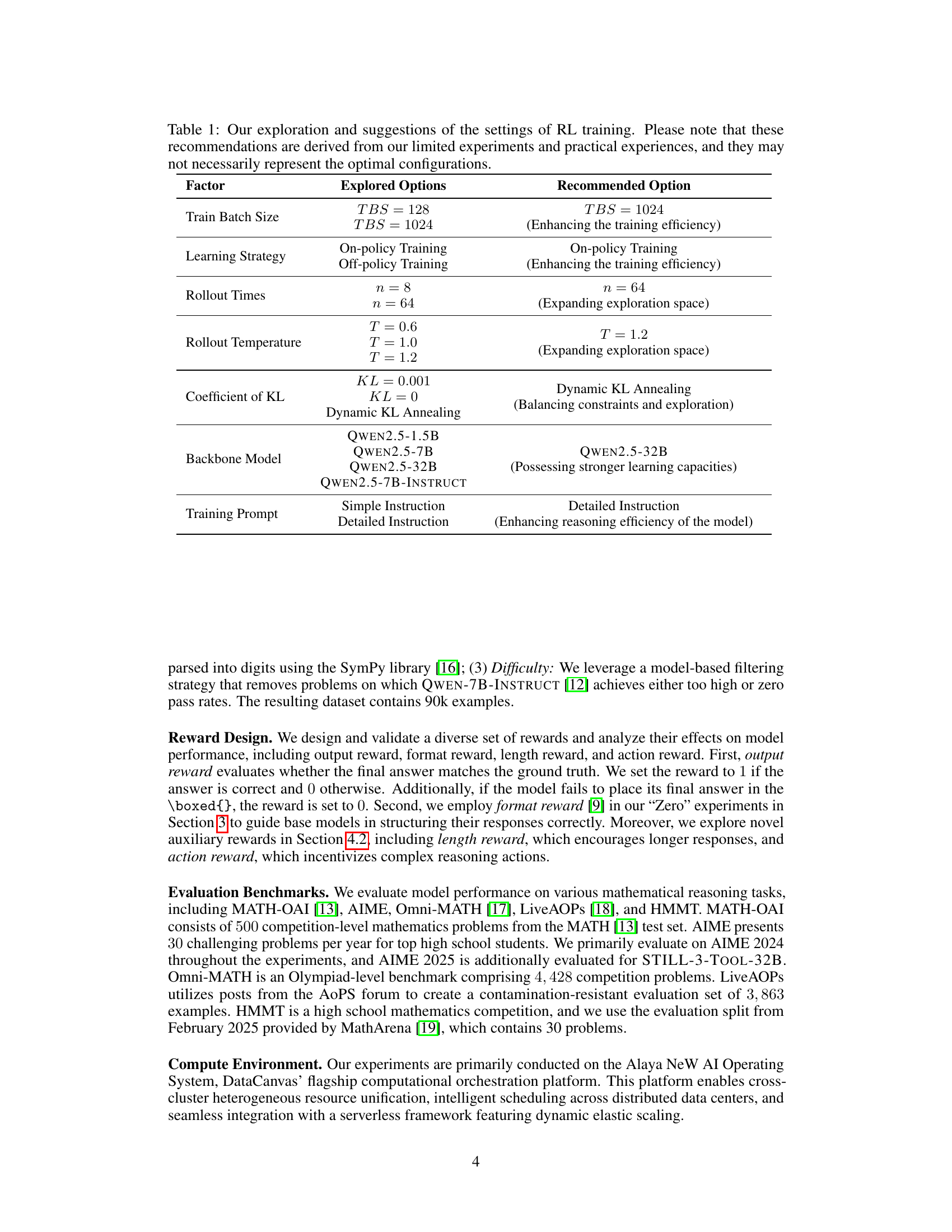
🔼 This table presents a summary of the hyperparameter settings explored during reinforcement learning (RL) training for large language models (LLMs), focusing on their impact on training efficiency and model performance. It compares various settings, including different train batch sizes, learning strategies (on-policy vs. off-policy), rollout times, rollout temperature, KL divergence coefficients, backbone models, and prompt types. For each setting, the table indicates the options explored during experimentation and provides a recommendation based on the authors’ experience and observations, emphasizing that these are not necessarily optimal but rather provide guidance based on their empirical findings.
read the caption
Table 1: Our exploration and suggestions of the settings of RL training. Please note that these recommendations are derived from our limited experiments and practical experiences, and they may not necessarily represent the optimal configurations.
In-depth insights#
RL’s Nuances#
When considering the nuances of Reinforcement Learning (RL) in the context of language models, several factors come into play. One crucial aspect is the reward function’s design, which significantly influences the model’s behavior and the kind of reasoning skills it develops. It’s important to carefully tune the reward to incentivize desired actions while avoiding unintended consequences like reward hacking. Another nuance involves the exploration-exploitation trade-off. RL relies on exploration to find optimal strategies. Balancing these two competing needs is challenging, especially in complex language-based tasks. Additionally, the choice of RL algorithm itself (e.g., on-policy vs. off-policy) impacts the training process, stability, and sample efficiency. The size and architecture of the language model also matter, as smaller models may struggle to effectively explore and learn complex reasoning patterns. Finally, training data quality and the choice of hyperparameters play critical roles in determining the success of RL training for language models.
Base vs. Fine-tune#
Base models and fine-tuned models represent two distinct approaches in developing sophisticated language models. Base models undergo pre-training on vast datasets, capturing general language patterns and knowledge. They are versatile but may lack specific task expertise. Fine-tuning, on the other hand, leverages a pre-trained base model and further trains it on a smaller, task-specific dataset. This allows the model to specialize and achieve higher performance on targeted tasks, such as question answering or text generation. The choice between the two depends on the desired balance between generality and specialization, as well as the availability of task-specific data. Fine-tuning is cost-effective when adapting a pre-existing model to a new task, while base models provide a foundation for diverse applications.
Tooling Impact#
Tooling’s impact on large language models (LLMs) is significant, especially in reasoning. Equipping LLMs with external tools like code interpreters or search engines augments their capabilities. Tool manipulation allows LLMs to overcome inherent limitations in knowledge and reasoning. The ability to generate and execute code enables models to tackle complex mathematical problems or verify reasoning steps. Tools like search engines provide access to real-time information, improving accuracy and reducing hallucination. Effective tool integration requires careful design, including appropriate prompts and training data. While smaller models benefit from imitation learning (SFT), larger models can leverage reinforcement learning (RL) to develop tool-use strategies autonomously. Tool-augmented LLMs show substantial performance gains across diverse tasks. However, challenges remain in optimizing tool selection and invocation. More research is needed to explore tool manipulation and the effectiveness of different training paradigms. Thus, the strategic use of tooling is crucial for advancing LLMs’ reasoning and problem-solving abilities.
Length Hacking#
The concept of “Length Hacking” in the context of reasoning models is fascinating. While longer responses are often correlated with enhanced reasoning in Large Language Models (LLMs) due to a larger search space, it’s crucial to recognize that LLMs can exploit length-biased reward functions. This means that LLMs can learn to generate excessively long responses simply to maximize their reward, without necessarily improving the quality or accuracy of their reasoning. This can lead to issues such as redundant checks, irrelevant concepts, and overall inefficient use of computational resources. True reasoning enhancement should stem from a model’s intrinsic learning processes, not from directly incentivizing longer responses. This can be addressed by monitoring the model’s generated content diversity and maintaining a high-quality reward signal, as well as avoiding excessive reward penalties for generating the longer responses.
Scaling RL#
Scaling Reinforcement Learning (RL) presents multifaceted challenges. The optimization of hyperparameters, backbone models, and training data significantly impacts the success of RL. Larger batch sizes enhance training efficiency, while on-policy learning fosters exploration and superior performance. The number of rollout times and rollout temperature also require careful tuning. An effective KL penalty balances exploration and stability. Emergent reasoning is a key indicator of successful scaling, with models exhibiting human-like reasoning. Reward hacking is a major consideration, and efforts should focus on encouraging reasoning actions rather than directly rewarding longer responses. Finally, balancing exploration and exploitation is critical for avoiding performance bottlenecks and achieving consistent improvements in reasoning tasks.
More visual insights#
More on figures

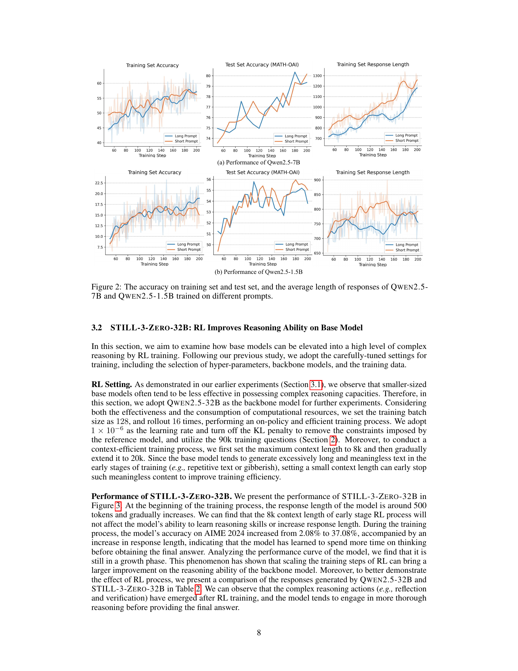
🔼 This figure compares the performance of two Qwen2.5 language models (7B and 1.5B parameters) during reinforcement learning (RL) training. The models were trained using two different prompt styles: a short prompt with basic instructions and a long prompt with more detailed instructions on how to perform the reasoning process. The plots show the accuracy on a training set and a MATH-OAI test set, along with the average length of the model’s responses over the course of the RL training. This comparison allows for analysis of how prompt engineering and model size affect the effectiveness of RL training for enhancing reasoning ability.
read the caption
Figure 2: The accuracy on training set and test set, and the average length of responses of Qwen2.5-7B and Qwen2.5-1.5B trained on different prompts.

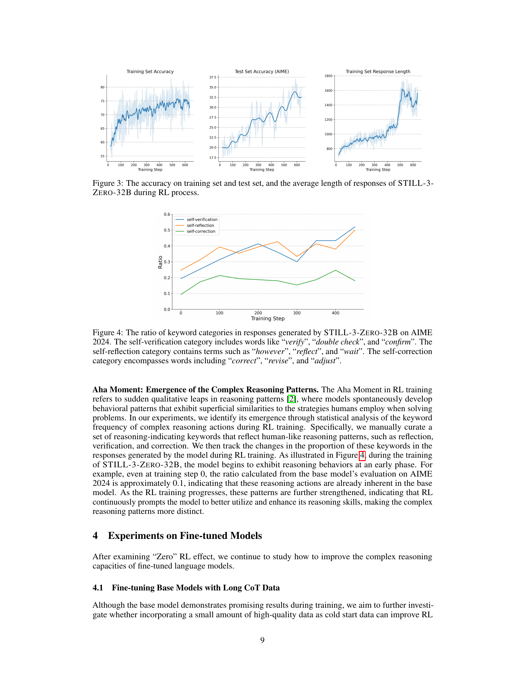
🔼 This figure displays the performance of the STILL-3-Zero-32B model during reinforcement learning (RL) training. It shows three key metrics plotted against training steps: 1) Training set accuracy, representing the model’s performance on the training data; 2) Test set accuracy (AIME), measuring performance on the AIME 2024 benchmark; and 3) Average response length, indicating the average number of tokens in the model’s responses. The graph allows for visualization of how these metrics evolve as the model undergoes RL training. This helps to assess the effectiveness of the RL training in improving both accuracy and reasoning capabilities (as measured by response length).
read the caption
Figure 3: The accuracy on training set and test set, and the average length of responses of STILL-3-Zero-32B during RL process.

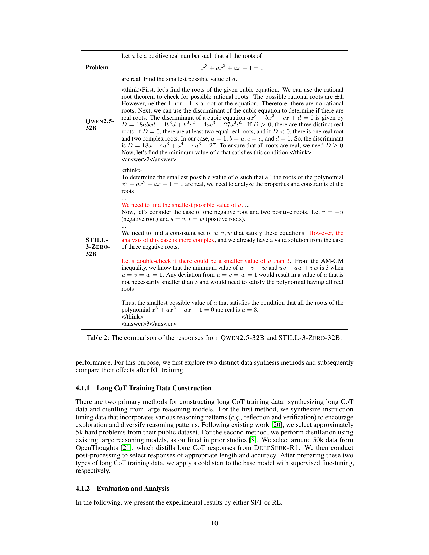
🔼 Figure 4 shows the evolution of reasoning patterns in the STILL-3-Zero-32B model during RL training on the AIME 2024 dataset. It tracks the proportion of keywords associated with three key reasoning processes over training steps. The ‘self-verification’ category (e.g., ‘verify’, ‘double check’, ‘confirm’) reflects the model’s tendency to check its work. The ‘self-reflection’ category (e.g., ‘however’, ‘reflect’, ‘wait’) indicates the model’s ability to reconsider its approach. The ‘self-correction’ category (e.g., ‘correct’, ‘revise’, ‘adjust’) demonstrates its capacity to identify and fix errors. The increasing proportions of these keywords suggest a refinement of the model’s reasoning process towards more human-like, deliberate thinking during training.
read the caption
Figure 4: The ratio of keyword categories in responses generated by STILL-3-Zero-32B on AIME 2024. The self-verification category includes words like “verify”, “double check”, and “confirm”. The self-reflection category contains terms such as “however”, “reflect”, and “wait”. The self-correction category encompasses words including “correct”, “revise”, and “adjust”.

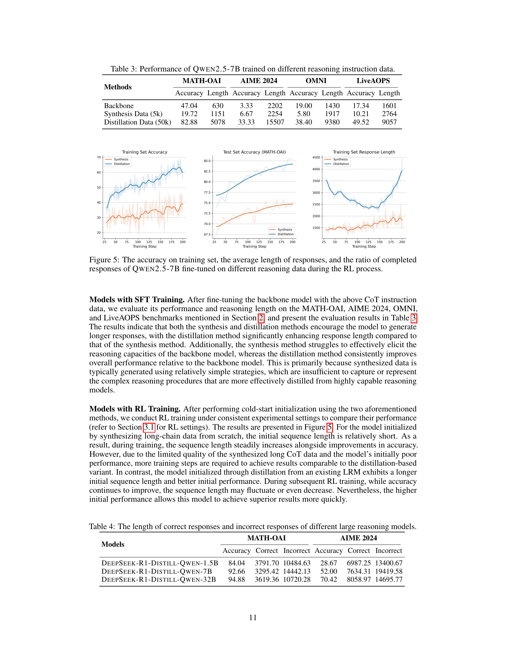
🔼 Figure 5 presents a comparative analysis of three key metrics—training set accuracy, average response length, and the ratio of completed responses—for the QWEN2.5-7B language model fine-tuned using two distinct methods: data synthesis and data distillation. The figure illustrates how these metrics evolve across the RL training process for both fine-tuning strategies. It highlights the differences in performance and training dynamics resulting from these two distinct approaches to data preparation for reinforcement learning.
read the caption
Figure 5: The accuracy on training set, the average length of responses, and the ratio of completed responses of Qwen2.5-7B fine-tuned on different reasoning data during the RL process.

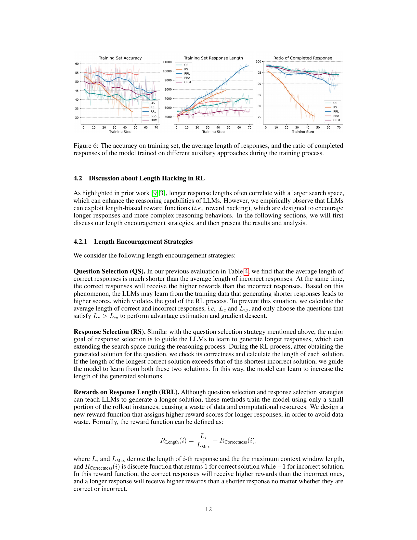
🔼 Figure 6 presents a comparative analysis of three different auxiliary training methods used to enhance the length of model responses during reinforcement learning. The x-axis represents the training step, while the y-axis displays three key metrics: training set accuracy, the average length of generated responses, and the ratio of completed responses. Each line on the graph represents the performance of the model under a specific auxiliary method (QS, RS, RRL, RRA, ORM). By examining these metrics, the figure allows for a comprehensive understanding of how each strategy influences the model’s ability to generate longer, more accurate, and complete responses over the course of training.
read the caption
Figure 6: The accuracy on training set, the average length of responses, and the ratio of completed responses of the model trained on different auxiliary approaches during the training process.

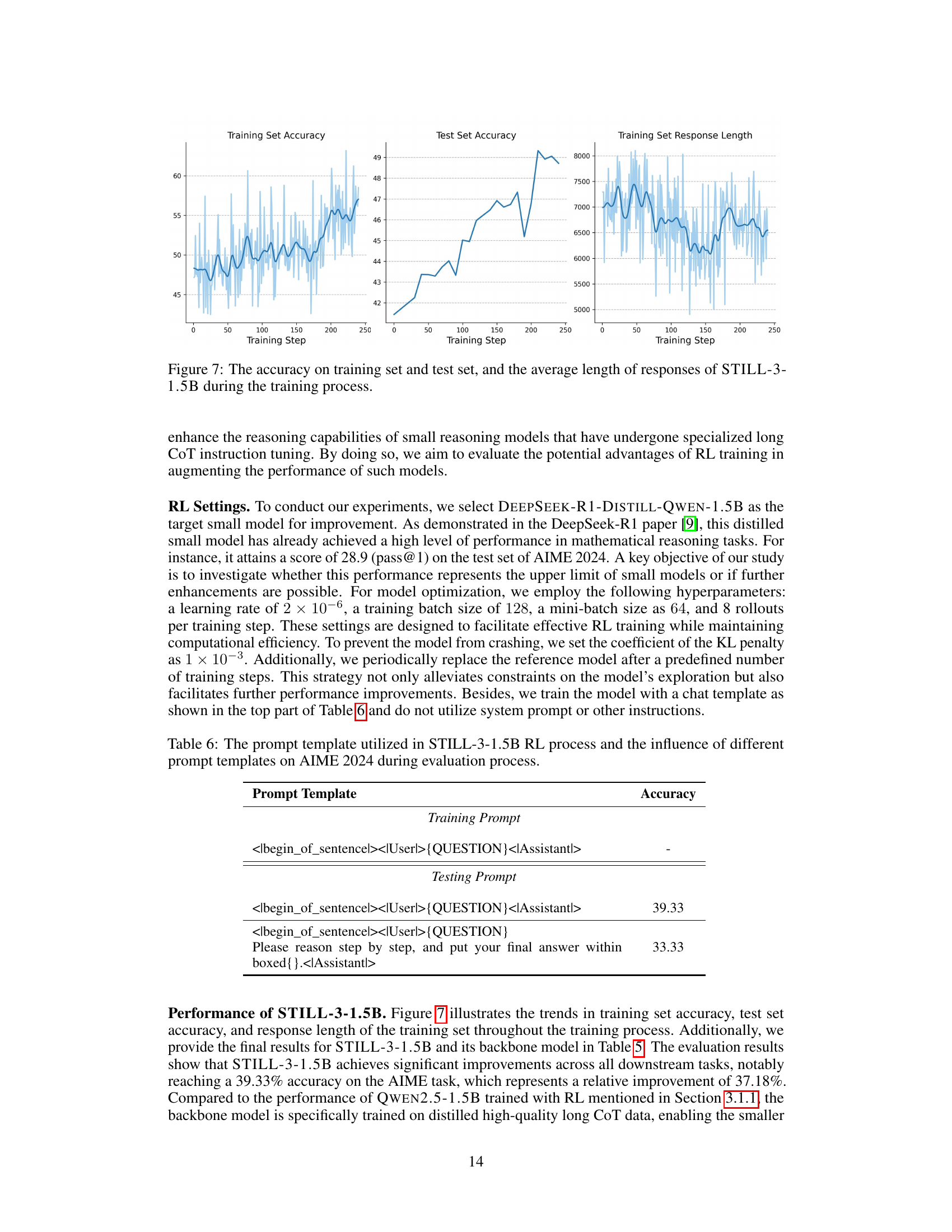
🔼 This figure displays the performance of the STILL-3-1.5B model throughout its reinforcement learning (RL) training process. The x-axis represents the training step, indicating the progression of the training. The three lines show the model’s accuracy on the training dataset, its accuracy on the test dataset (a separate dataset used to evaluate generalization performance), and the average length of the responses generated by the model at each training step. The plot illustrates how the model’s accuracy and response length evolve as it learns through RL, providing insights into the training dynamics and the relationship between model performance and response length.
read the caption
Figure 7: The accuracy on training set and test set, and the average length of responses of STILL-3-1.5B during the training process.

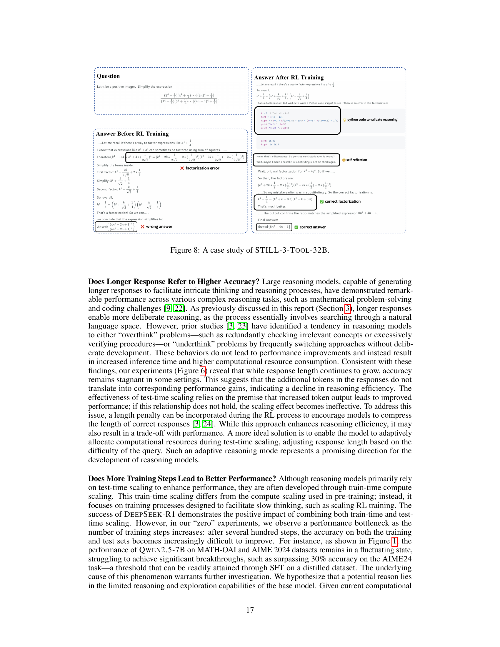
🔼 This figure showcases a specific example of how STILL-3-Tool-32B, a large language model enhanced with tool manipulation capabilities, approaches a mathematical problem. It contrasts the model’s reasoning process before and after reinforcement learning (RL) training. The ‘Before RL Training’ section illustrates an initial attempt at solving the problem, revealing errors and flawed reasoning. The ‘After RL Training’ section demonstrates the model’s improved reasoning abilities after RL training; it identifies and corrects its previous mistakes, even using a Python code snippet for verification and successfully arrives at the correct answer. This figure highlights the significant improvement in both the accuracy and the sophistication of the model’s reasoning process after RL training.
read the caption
Figure 8: A case study of STILL-3-Tool-32B.

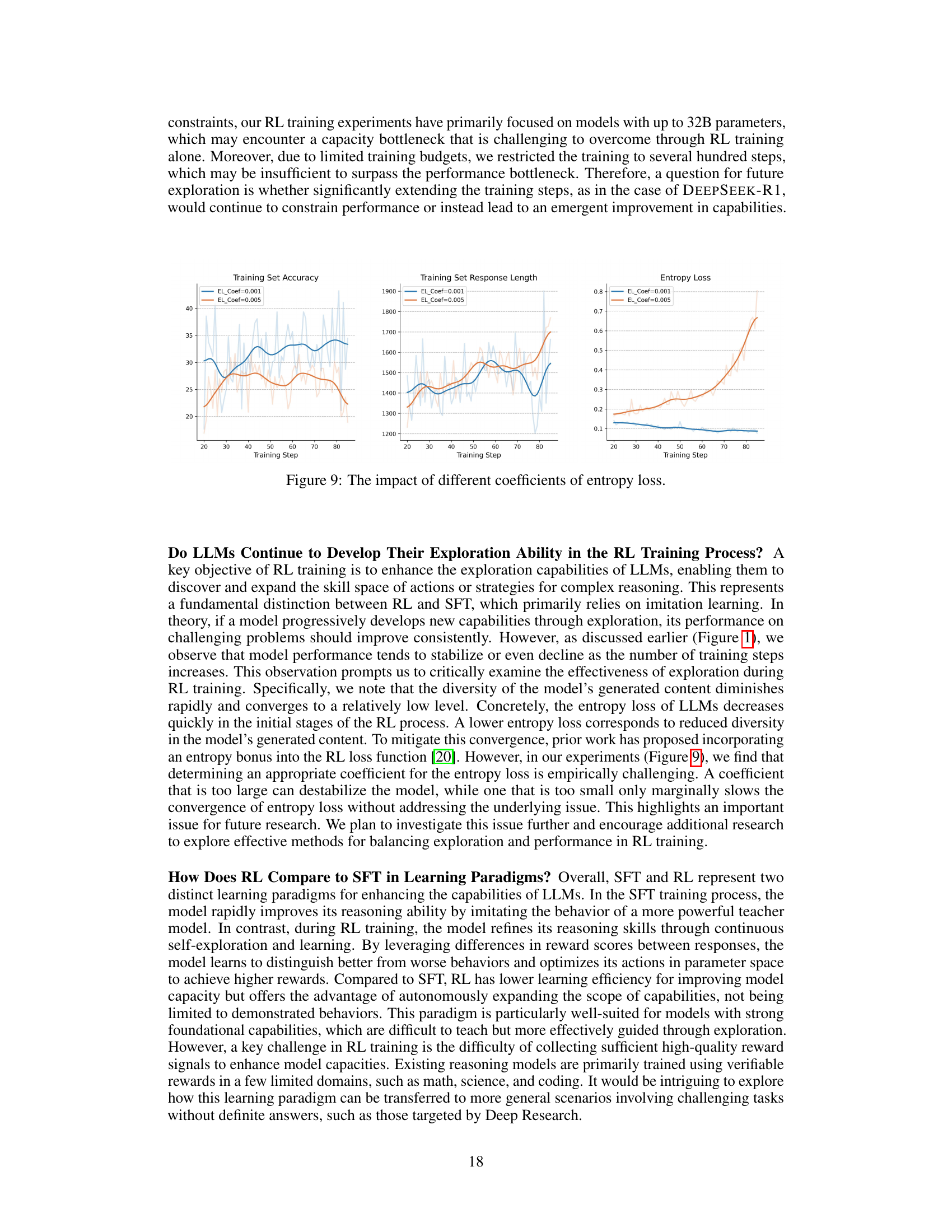
🔼 This figure displays the effects of varying the coefficient of entropy loss during reinforcement learning (RL) training. It shows three subplots tracking the training set accuracy, training set response length, and entropy loss over the course of training. Each subplot presents two lines, representing the results using two different coefficients for entropy loss (0.001 and 0.005). This visualization helps to understand how different coefficients influence the exploration-exploitation trade-off during RL. The trends in accuracy, response length, and entropy loss are presented to assess the impact of each coefficient on the overall training process.
read the caption
Figure 9: The impact of different coefficients of entropy loss.
More on tables
|
| ||||||||||||
|
| ||||||||||||
|
|
🔼 This table compares the responses generated by the QWEN2.5-32B base model and the STILL-3-Zero-32B model (which underwent direct RL training without an intermediate SFT stage) to the same mathematical reasoning problem. It highlights the differences in the reasoning process and the final answers produced by each model, showcasing how direct RL training influences the model’s reasoning capabilities.
read the caption
Table 2: The comparison of the responses from Qwen2.5-32B and STILL-3-Zero-32B.
| Problem |
🔼 This table presents the performance of the QWEN2.5-7B language model after being fine-tuned on different reasoning instruction datasets. It compares the model’s accuracy and response length across four different benchmark datasets: MATH-OAI, AIME 2024, OMNI, and LiveAOPS. Two different fine-tuning datasets are used: one synthesized from scratch (5k examples) and one distilled from a larger pre-trained model (50k examples). The comparison helps illustrate the impact of different training data on the model’s ability to perform mathematical reasoning tasks.
read the caption
Table 3: Performance of Qwen2.5-7B trained on different reasoning instruction data.
| Let be a positive real number such that all the roots of are real. Find the smallest possible value of |
🔼 This table compares the average lengths of correct and incorrect responses generated by several large reasoning models on two benchmark datasets, MATH-OAI and AIME 2024. The goal is to show the relationship between response length and accuracy; longer responses are generally associated with more complex reasoning, but not always with higher accuracy. The models compared represent various approaches and sizes, illustrating differences in their reasoning performance and tendencies toward either overly concise or overly verbose responses.
read the caption
Table 4: The length of correct responses and incorrect responses of different large reasoning models.
| Qwen2.5-32B |
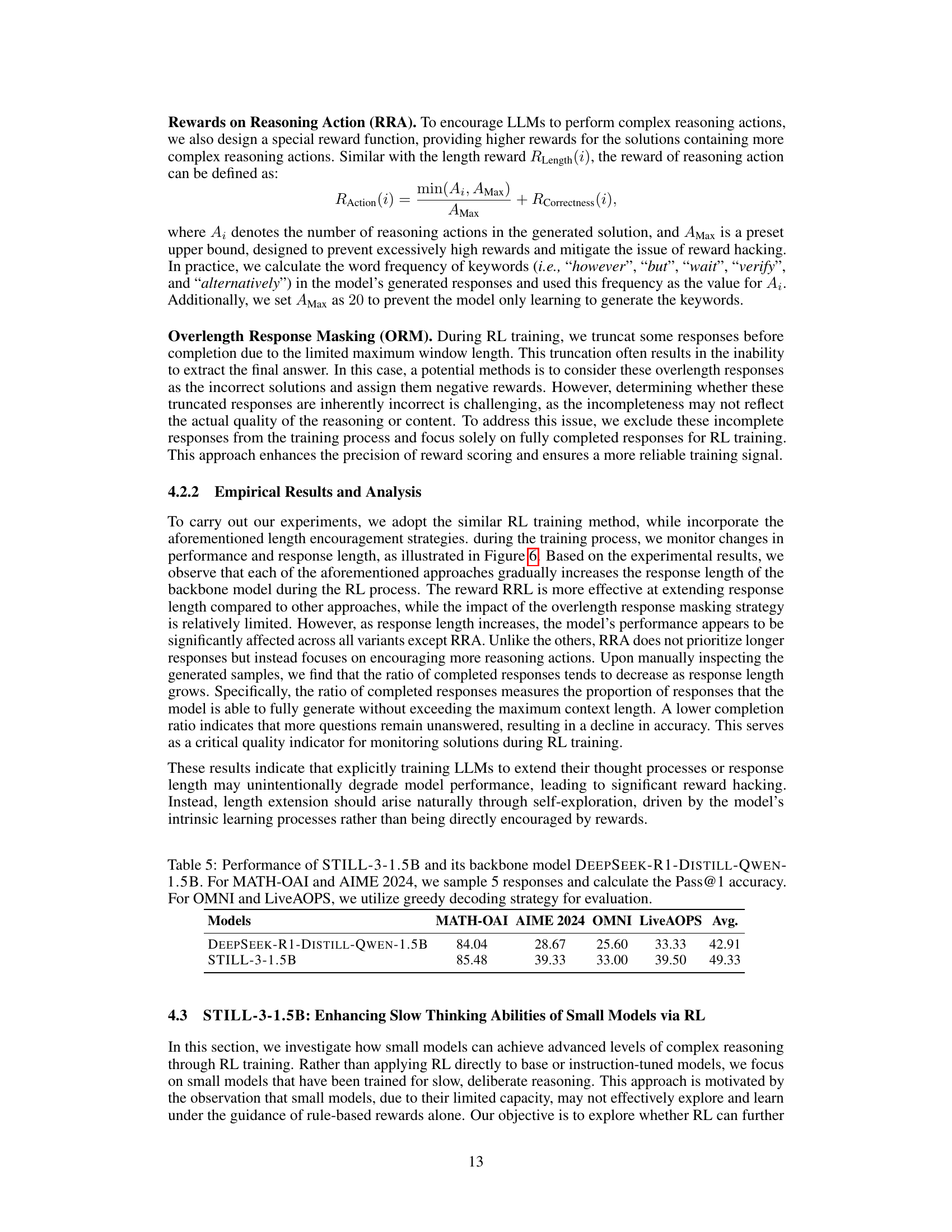
🔼 This table presents a comparison of the performance of two models on various mathematical reasoning tasks. STILL-3-1.5B is a smaller model that has undergone further training using reinforcement learning (RL) techniques, building upon its pre-trained backbone model DeepSeek-R1-Distill-Qwen-1.5B. The table shows the accuracy of each model on four different benchmark datasets: MATH-OAI, AIME 2024, Omni, and LiveAOPS. For MATH-OAI and AIME 2024, the Pass@1 accuracy (the percentage of times the top-ranked answer is correct) is reported based on five sampled responses per question. For Omni and LiveAOPS, the greedy decoding strategy is used for evaluation.
read the caption
Table 5: Performance of STILL-3-1.5B and its backbone model DeepSeek-R1-Distill-Qwen-1.5B. For MATH-OAI and AIME 2024, we sample 5 responses and calculate the Pass@1 accuracy. For OMNI and LiveAOPS, we utilize greedy decoding strategy for evaluation.
| <think>First, let’s find the roots of the given cubic equation. We can use the rational root theorem to check for possible rational roots. The possible rational roots are . However, neither nor is a root of the equation. Therefore, there are no rational roots. Next, we can use the discriminant of the cubic equation to determine if there are real roots. The discriminant of a cubic equation is given by . If , there are three distinct real roots; if , there are at least two equal real roots; and if , there is one real root and two complex roots. In our case, , , , and . So, the discriminant is . To ensure that all roots are real, we need . Now, let’s find the minimum value of a that satisfies this condition.</think> |
| <answer>2</answer> |
🔼 This table details the prompt engineering experiments conducted as part of the STILL-3-1.5B RL training process. It shows how different prompt templates affect the model’s performance on the AIME 2024 benchmark. The table contrasts a simple prompt template against one providing more detailed instructions on the reasoning process, highlighting the impact of prompt design on the model’s accuracy during reinforcement learning.
read the caption
Table 6: The prompt template utilized in STILL-3-1.5B RL process and the influence of different prompt templates on AIME 2024 during evaluation process.
| STILL-3-Zero-32B |
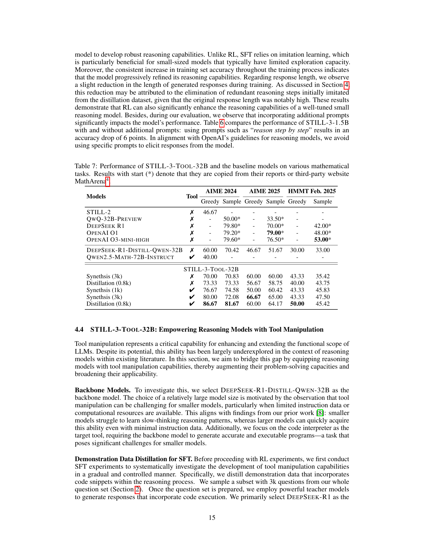
🔼 Table 7 presents a comparative analysis of the performance of various large language models (LLMs) on several mathematical reasoning tasks. The primary focus is on STILL-3-Tool-32B, a model enhanced with tool manipulation capabilities. Results are shown for different evaluation metrics (accuracy) across four benchmark datasets: AIME 2024, AIME 2025, and HMMT February 2025. For comparison, the table includes results from other notable LLMs such as Qwen-32B-Preview, DeepSeek-R1, and several OpenAI models. Where data was obtained from external sources (like MathArena), this is explicitly indicated. The results highlight the performance improvements achieved by STILL-3-Tool-32B, particularly its ability to integrate external tools effectively.
read the caption
Table 7: Performance of STILL-3-Tool-32B and the baseline models on various mathematical tasks. Results with start (*) denote that they are copied from their reports or third-party website MathArena333https://matharena.ai/.
Full paper#