TL;DR#
Large language models require scalable training approaches. Linear Sequence Modeling (LSM) and Mixture-of-Experts (MoE) are promising architectural improvements. However, attention layers rely on softmax, leading to quadratic complexity with input sequence length. LSM has emerged to achieve impressive efficiency with linear training and constant memory inference, and can be expressed with matrix-valued hidden states, similar to RNN.
This paper introduces Linear-MoE, production-level system that combines LSM with MoE for large-scale models. Linear-MoE has modeling and training subsystems with linear attention, state space models, and linear RNN. Incorporating sequence parallelism enhances training. Evaluations show that Linear-MoE achieves efficiency while maintaining competitive performance.
Key Takeaways#
Why does it matter?#
This paper is important for researchers, because it addresses the growing need for efficient and scalable training of large language models. By integrating LSMs with MoE, it opens new avenues for architectural innovation and efficient handling of long sequences. The exploration of hybrid models also provides valuable insights for future research.
Visual Insights#

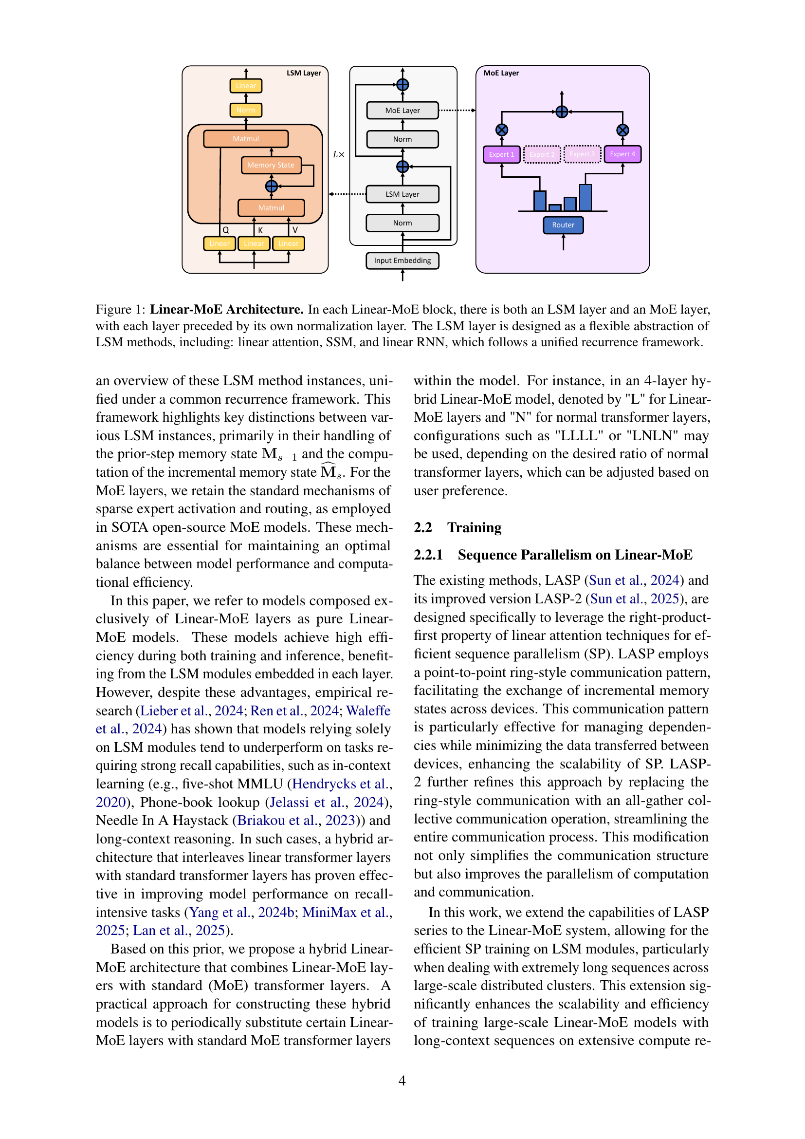
🔼 The Linear-MoE architecture consists of stacked Linear-MoE blocks. Each block contains a normalization layer followed by an LSM layer and an MoE layer. The LSM layer is a flexible module that unifies different linear sequence modeling methods such as linear attention, state space models, and linear RNNs under a common recurrence framework. The MoE layer implements the standard mixture-of-experts mechanism for sparse activation.
read the caption
Figure 1: Linear-MoE Architecture. In each Linear-MoE block, there is both an LSM layer and an MoE layer, with each layer preceded by its own normalization layer. The LSM layer is designed as a flexible abstraction of LSM methods, including: linear attention, SSM, and linear RNN, which follows a unified recurrence framework.
| LSM Method | Instance | Recurrent Update Rule | Parameter |
| Linear Attention | BLA | ||
| Lightning Attn | |||
| RetNet | |||
| GLA | |||
| DeltaNet | |||
| Rebased | |||
| GFW | |||
| GateLoop | |||
| Gated DeltaNet | |||
| TTT | |||
| Titans | |||
| SSM * | S4 | ||
| Mamba | |||
| Mamba2 | |||
| HGRN2 | |||
| Linear RNN | RWKV6 | ||
| RWKV7 |
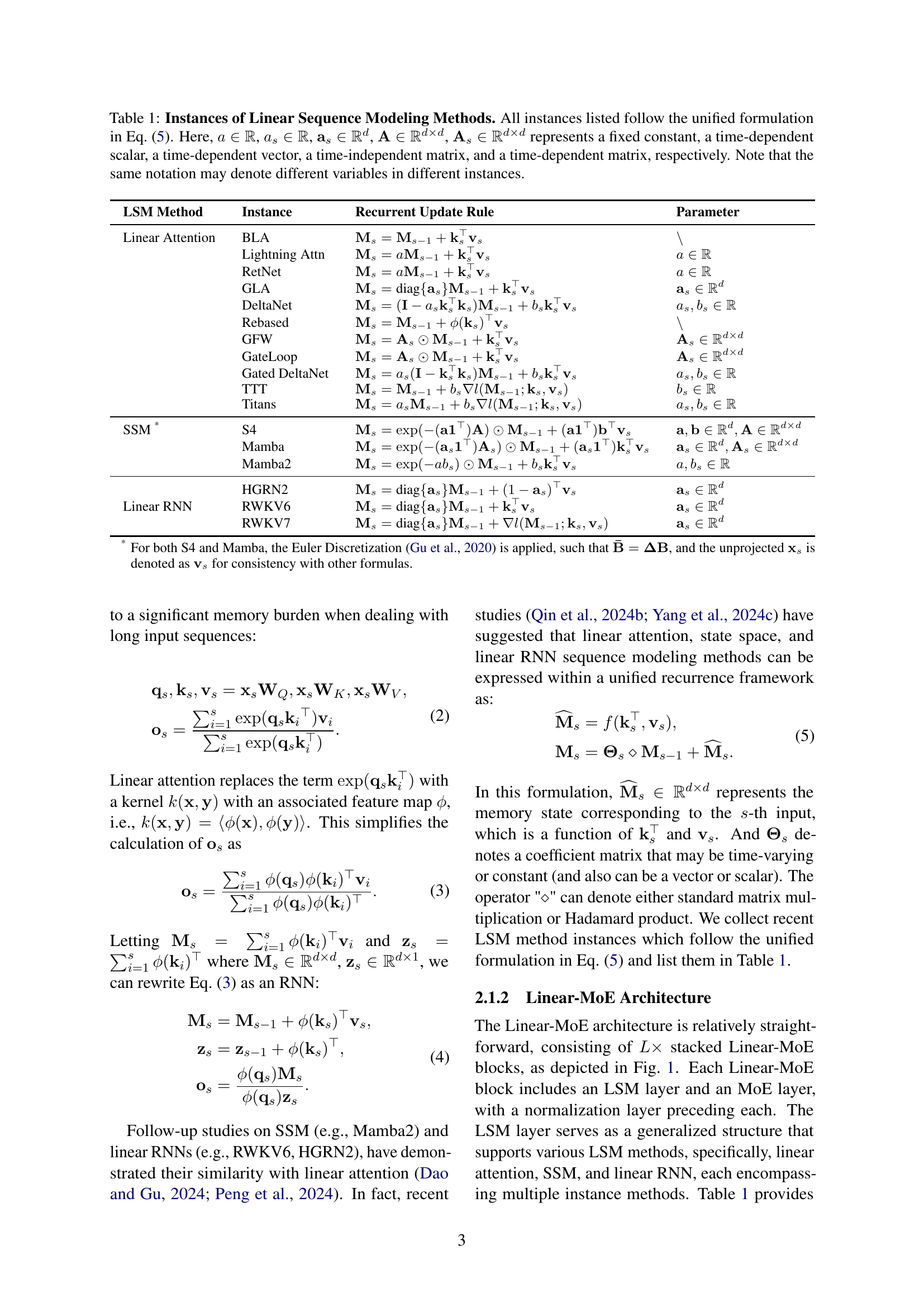
🔼 This table lists various instances of linear sequence modeling (LSM) methods. Each method is described by a recurrent update rule, which shows how the memory state is updated at each time step. The parameters (a, as, as, A, As) in the update rule represent a fixed constant, a time-dependent scalar, a time-dependent vector, a time-independent matrix, and a time-dependent matrix, respectively. All the LSM methods listed in the table share a common mathematical foundation and can be represented using the unified formulation presented in Equation 5 of the paper. Note that some symbols may represent different variables across different methods.
read the caption
Table 1: Instances of Linear Sequence Modeling Methods. All instances listed follow the unified formulation in Eq. (5). Here, a∈ℝ𝑎ℝa\in\mathbb{R}italic_a ∈ blackboard_R, as∈ℝsubscript𝑎𝑠ℝa_{s}\in\mathbb{R}italic_a start_POSTSUBSCRIPT italic_s end_POSTSUBSCRIPT ∈ blackboard_R, 𝐚s∈ℝdsubscript𝐚𝑠superscriptℝ𝑑\mathbf{a}_{s}\in\mathbb{R}^{d}bold_a start_POSTSUBSCRIPT italic_s end_POSTSUBSCRIPT ∈ blackboard_R start_POSTSUPERSCRIPT italic_d end_POSTSUPERSCRIPT, 𝐀∈ℝd×d𝐀superscriptℝ𝑑𝑑\mathbf{A}\in\mathbb{R}^{d\times d}bold_A ∈ blackboard_R start_POSTSUPERSCRIPT italic_d × italic_d end_POSTSUPERSCRIPT, 𝐀s∈ℝd×dsubscript𝐀𝑠superscriptℝ𝑑𝑑\mathbf{A}_{s}\in\mathbb{R}^{d\times d}bold_A start_POSTSUBSCRIPT italic_s end_POSTSUBSCRIPT ∈ blackboard_R start_POSTSUPERSCRIPT italic_d × italic_d end_POSTSUPERSCRIPT represents a fixed constant, a time-dependent scalar, a time-dependent vector, a time-independent matrix, and a time-dependent matrix, respectively. Note that the same notation may denote different variables in different instances.
In-depth insights#
Linear-MoE Intro#
Linear-MoE emerges as a novel architecture, integrating Linear Sequence Modeling (LSM) and Mixture-of-Experts (MoE). LSM offers linear complexity and efficient training, while MoE provides sparse activation. This combination aims for high performance with efficient resource utilization, addressing the quadratic complexity of standard attention. The system encompasses modeling and training subsystems, supporting various LSM instances (linear attention, SSM, linear RNN) under a unified framework. Sequence Parallelism is designed for efficient long-sequence processing. Hybrid models combining Linear-MoE and Transformer-MoE layers enhance flexibility. Evaluations demonstrate efficiency gains while maintaining competitive performance.
Unified LSM System#
The concept of a unified LSM (Linear Sequence Model) system is intriguing. The primary goal is to provide a singular framework that can accommodate a variety of LSM implementations, such as linear attention, SSMs (State Space Models), and linear RNNs (Recurrent Neural Networks). This unification offers significant advantages, as it simplifies the development and experimentation with different LSM architectures. A unified system likely involves defining a set of common interfaces and abstractions that all LSM implementations must adhere to, enabling modularity and interchangeability. It can promote code reuse and facilitate the comparison of different LSMs under controlled conditions. Ideally, the unified system would encapsulate the core operations of LSMs while allowing for customization through configurable parameters or plugin-like extensions. Such standardization might lead to the creation of more robust and versatile sequence models.
Hybrid Model SP#
The concept of ‘Hybrid Model SP’ likely refers to a parallel processing strategy tailored for models combining different architectural elements. It probably involves splitting the model across multiple devices, optimizing communication between them. A crucial aspect might be balancing the workload between different types of layers or sub-networks within the hybrid model, requiring careful consideration of computational demands and data dependencies. The ‘SP’ component likely indicates sequence parallelism, suggesting that the input sequence is divided and processed concurrently, with appropriate mechanisms for maintaining dependencies and ensuring coherent output. Optimizing hybrid models is essential to exploit the unique characteristics of different model components.
Training Efficiency#
Training efficiency is critical for large language models. The paper likely investigates how incorporating linear sequence modeling (LSM) affects training throughput and memory usage compared to traditional methods like softmax attention. LSM aims for linear complexity, potentially enabling longer sequences. Expect discussion of hardware utilization (GPU), batch size, and sequence length’s impact on training. The authors probably benchmarked diverse LSM variants, highlighting their strengths and weaknesses in terms of memory footprint, computational cost, and scalability. Performance comparisons against baselines like standard attention and optimized implementations such as FlashAttention are anticipated, alongside ablations on the impact of parallelism strategies. Further investigations involving MoE optimization techniques such as grouped GEMM and MegaBlocks is expected, alongside exploration of diverse parallelism methods such as TP, DP, and SP.
Hybrid > Pure LSM#
The concept of “Hybrid > Pure LSM” suggests that models combining Linear Sequence Modeling (LSM) layers with standard Transformer layers often outperform models relying solely on LSM layers. Pure LSM models offer efficiency in training and inference due to their linear complexity, but may lack the strong recall capabilities of Transformers. This hybrid approach strategically balances the strengths of both architectures. By interleaving LSM layers (efficient sequence processing) with Transformer layers (superior memory and context handling), the hybrid models can achieve better performance on tasks requiring both efficiency and strong recall, such as long-context reasoning and in-context learning. The key is to leverage LSMs for speed and Transformers for accuracy, creating a more versatile and powerful model. This synergistic effect allows the model to adapt better to diverse tasks and data types, optimizing overall performance and addressing the limitations inherent in each individual architecture.
More visual insights#
More on figures

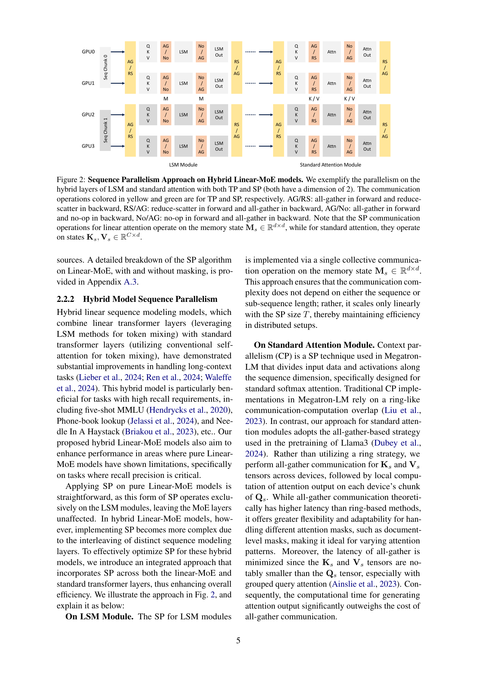
🔼 Figure 2 illustrates the sequence parallelism approach used in hybrid Linear-MoE models, which combine linear sequence modeling (LSM) layers and standard attention layers. The diagram shows how the computation is distributed across multiple GPUs (GPU0, GPU1, GPU2, GPU3) for both LSM and standard attention layers, using both tensor parallelism (TP) and sequence parallelism (SP), each with a dimension of 2. The colors yellow and green represent communication operations for TP and SP, respectively. Abbreviations AG, RS, and No represent all-gather, reduce-scatter, and no-op operations in the forward and backward passes. A key distinction is highlighted: sequence parallelism for linear attention operates on the memory state (a matrix of size d x d), whereas sequence parallelism for standard attention operates on the key (K) and value (V) matrices (matrices of size C x d). This difference reflects the distinct computational characteristics of the two types of layers.
read the caption
Figure 2: Sequence Parallelism Approach on Hybrid Linear-MoE models. We exemplify the parallelism on the hybrid layers of LSM and standard attention with both TP and SP (both have a dimension of 2). The communication operations colored in yellow and green are for TP and SP, respectively. AG/RS: all-gather in forward and reduce-scatter in backward, RS/AG: reduce-scatter in forward and all-gather in backward, AG/No: all-gather in forward and no-op in backward, No/AG: no-op in forward and all-gather in backward. Note that the SP communication operations for linear attention operate on the memory state 𝐌s∈ℝd×dsubscript𝐌𝑠superscriptℝ𝑑𝑑\mathbf{M}_{s}\in\mathbb{R}^{d\times d}bold_M start_POSTSUBSCRIPT italic_s end_POSTSUBSCRIPT ∈ blackboard_R start_POSTSUPERSCRIPT italic_d × italic_d end_POSTSUPERSCRIPT, while for standard attention, they operate on states 𝐊s,𝐕s∈ℝC×dsubscript𝐊𝑠subscript𝐕𝑠superscriptℝ𝐶𝑑\mathbf{K}_{s},\mathbf{V}_{s}\in\mathbb{R}^{C\times d}bold_K start_POSTSUBSCRIPT italic_s end_POSTSUBSCRIPT , bold_V start_POSTSUBSCRIPT italic_s end_POSTSUBSCRIPT ∈ blackboard_R start_POSTSUPERSCRIPT italic_C × italic_d end_POSTSUPERSCRIPT.

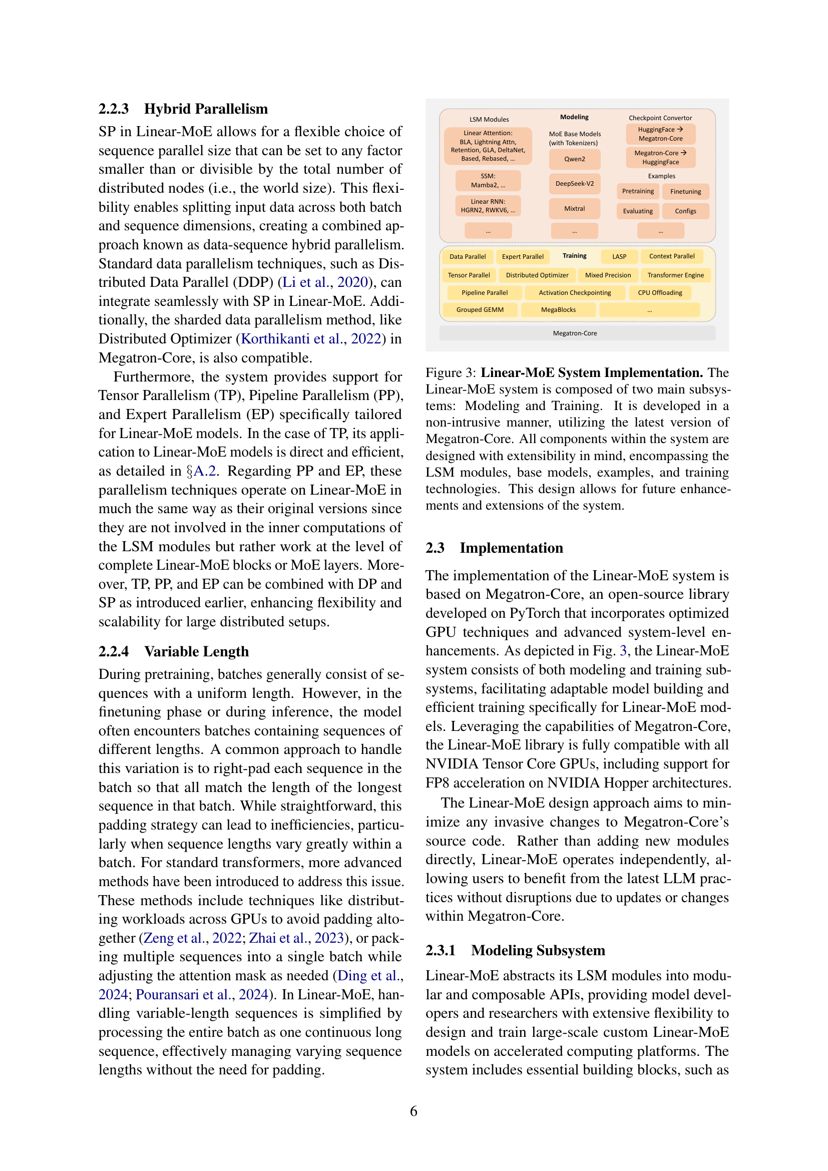
🔼 The Linear-MoE system is composed of two main subsystems: Modeling and Training. The Modeling subsystem provides a unified framework for various linear sequence modeling (LSM) methods, including linear attention, state space models, and linear RNNs. These LSM modules can be integrated with Mixture-of-Experts (MoE) layers. The Training subsystem facilitates efficient training by incorporating advanced parallelism technologies, particularly Sequence Parallelism. The figure illustrates the architecture, highlighting the modular and extensible design that allows for easy integration of new LSM methods, base models, and training techniques in the future. It leverages Megatron-Core for core functionalities.
read the caption
Figure 3: Linear-MoE System Implementation. The Linear-MoE system is composed of two main subsystems: Modeling and Training. It is developed in a non-intrusive manner, utilizing the latest version of Megatron-Core. All components within the system are designed with extensibility in mind, encompassing the LSM modules, base models, examples, and training technologies. This design allows for future enhancements and extensions of the system.

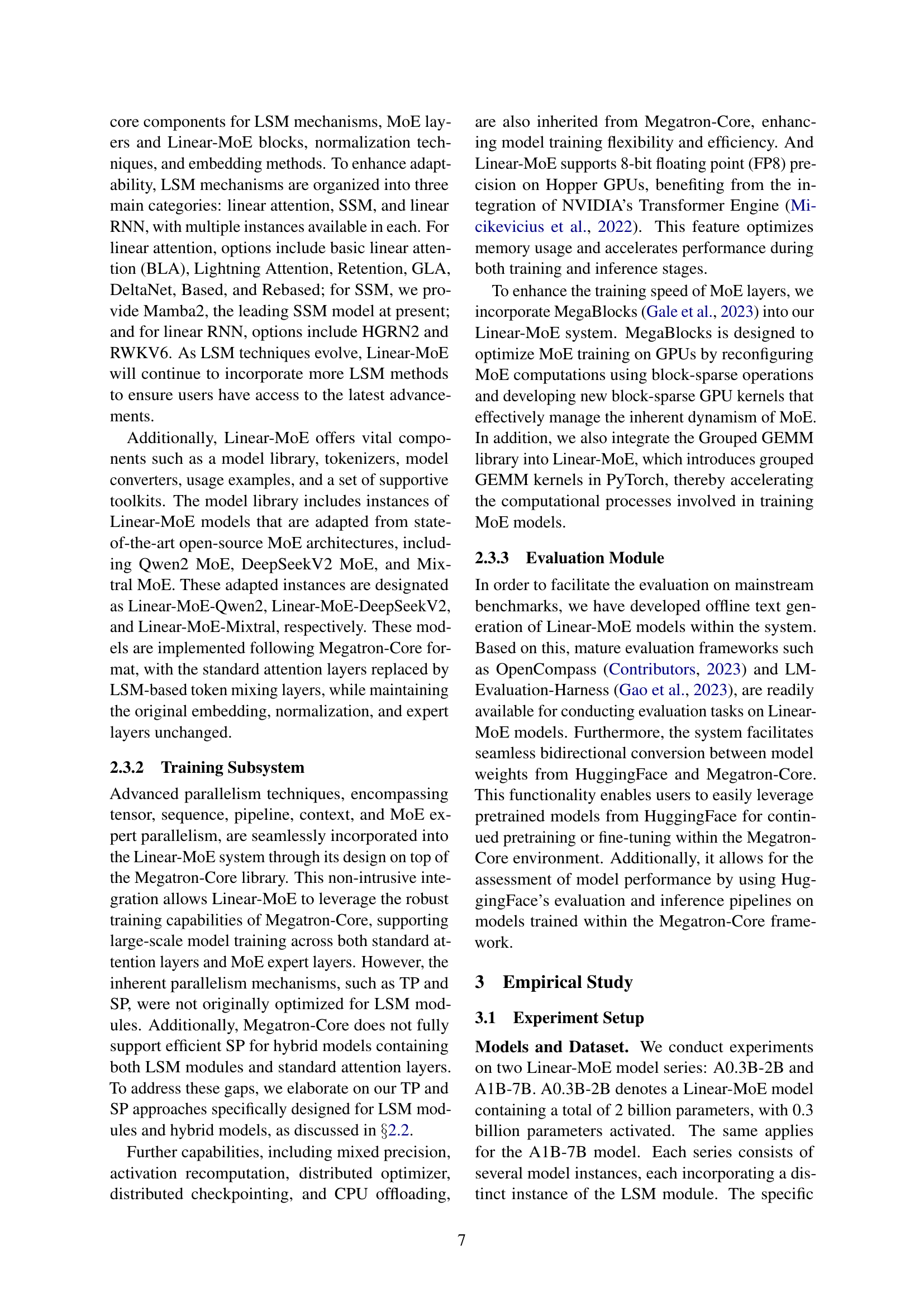
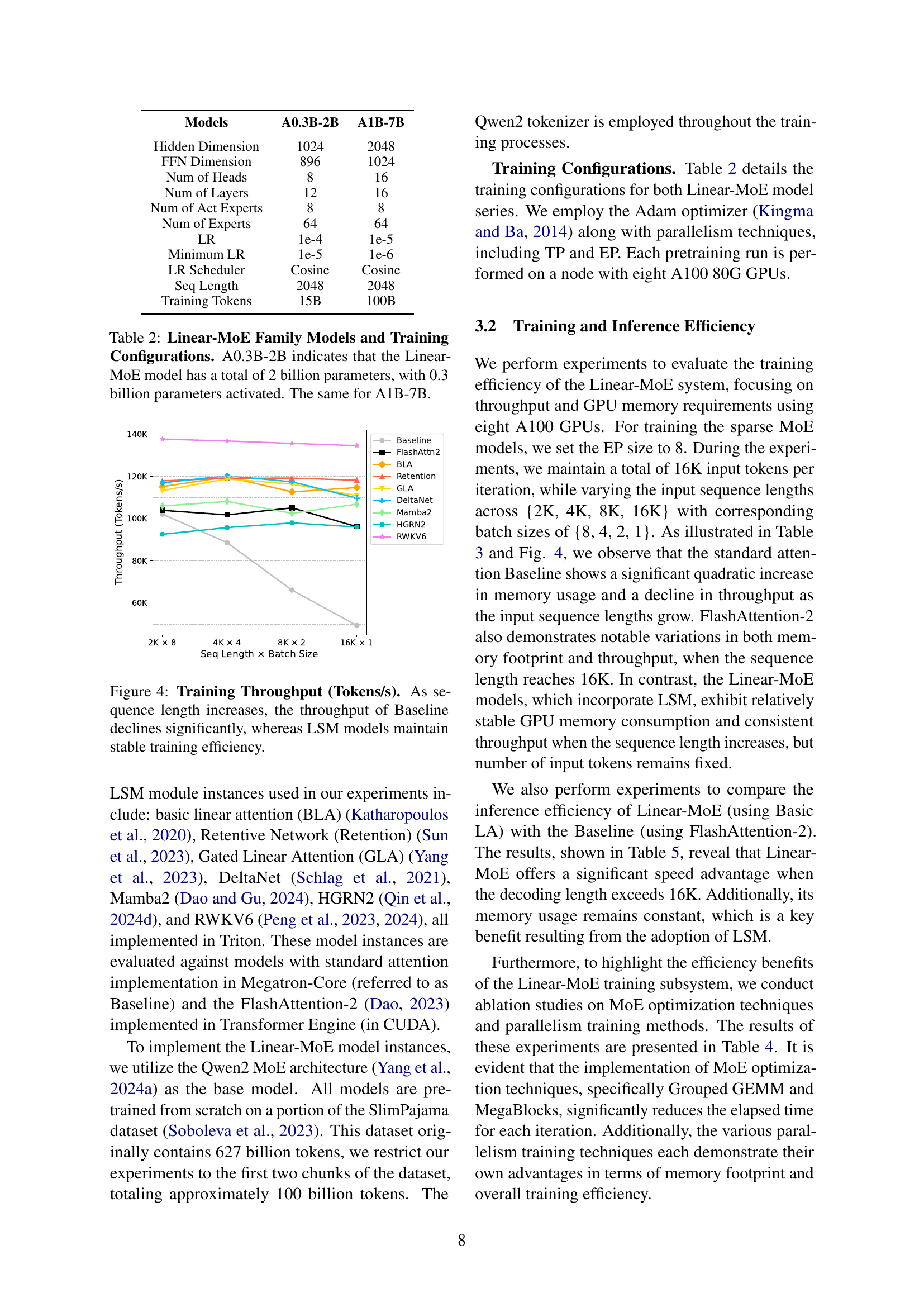
🔼 Figure 4 illustrates the training throughput, measured in tokens per second, for various models across different sequence lengths and batch sizes. The ‘Baseline’ model, which represents a standard Transformer model with softmax attention, shows a significant decrease in throughput as the sequence length increases. This illustrates the quadratic complexity of softmax attention. In contrast, Linear Sequence Modeling (LSM) methods demonstrate much more stable training throughput, even with longer sequence lengths. This highlights the advantage of LSM in maintaining efficient training, regardless of input sequence size.
read the caption
Figure 4: Training Throughput (Tokens/s). As sequence length increases, the throughput of Baseline declines significantly, whereas LSM models maintain stable training efficiency.

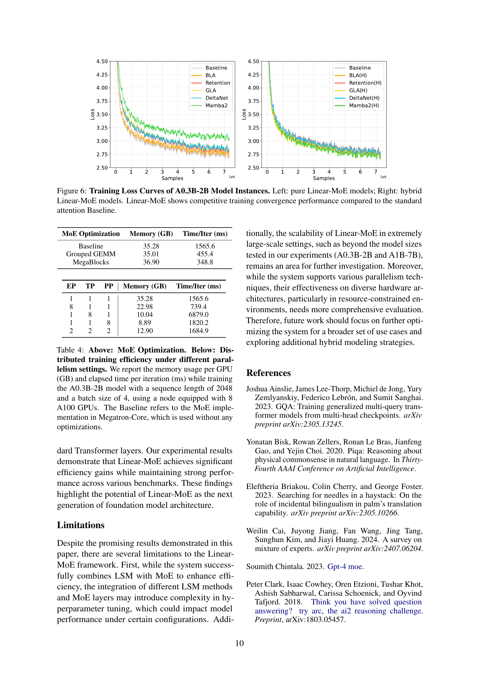
🔼 This figure compares the inference efficiency of two A0.3B-2B models: a baseline model using FlashAttention-2 and a Linear-MoE model using basic linear attention. Both models were tested on a single A800 80GB GPU with a fixed batch size of 16, while varying the decoding length from 1K to 128K tokens. The graph illustrates the trade-off between inference latency (time) and GPU memory usage for both models across different decoding lengths. This allows for a direct comparison of the performance and resource consumption of the two approaches for long sequence inference.
read the caption
Figure 5: Inference Efficiency of A0.3B-2B Model Instances. We variate the decoding length from 1K to 128K with fixed batch size of 16 on single A800 80GB GPU to evaluate the Baseline w/ FlashAttention-2 and the Linear-MoE w/ Basic Linear Attention in terms of inference latency time and GPU memory usage.

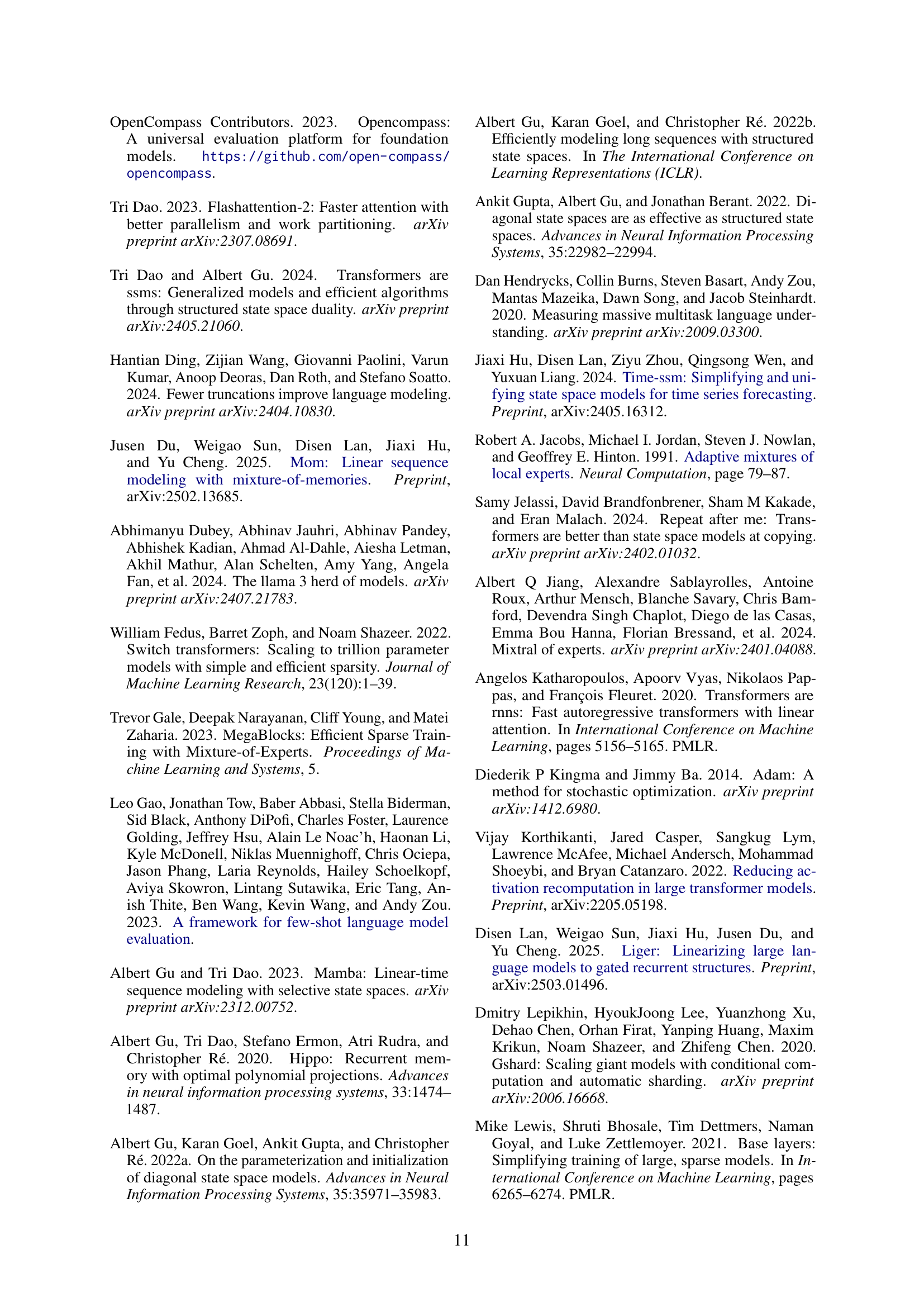
🔼 This figure displays the training loss curves for the A0.3B-2B Linear-MoE model. The left panel shows curves for models using only Linear-MoE layers, while the right panel presents curves for hybrid models which incorporate both Linear-MoE and standard Transformer-MoE layers. The comparison highlights that the Linear-MoE models demonstrate competitive training convergence performance when compared to the baseline model which utilizes standard attention mechanisms.
read the caption
Figure 6: Training Loss Curves of A0.3B-2B Model Instances. Left: pure Linear-MoE models; Right: hybrid Linear-MoE models. Linear-MoE shows competitive training convergence performance compared to the standard attention Baseline.
More on tables
| Models | A0.3B-2B | A1B-7B |
| Hidden Dimension | 1024 | 2048 |
| FFN Dimension | 896 | 1024 |
| Num of Heads | 8 | 16 |
| Num of Layers | 12 | 16 |
| Num of Act Experts | 8 | 8 |
| Num of Experts | 64 | 64 |
| LR | 1e-4 | 1e-5 |
| Minimum LR | 1e-5 | 1e-6 |
| LR Scheduler | Cosine | Cosine |
| Seq Length | 2048 | 2048 |
| Training Tokens | 15B | 100B |
🔼 This table details the configurations used for training two families of Linear-MoE models: A0.3B-2B and A1B-7B. The A0.3B-2B model has 2 billion parameters, of which 0.3 billion are activated during training. Similarly, A1B-7B has 7 billion parameters, with a portion activated during training. The table lists key hyperparameters for both models including hidden dimension, feedforward network (FFN) dimension, number of attention heads, number of layers, number of activated experts, number of total experts, learning rate (LR), minimum learning rate, learning rate scheduler, sequence length, and total training tokens.
read the caption
Table 2: Linear-MoE Family Models and Training Configurations. A0.3B-2B indicates that the Linear-MoE model has a total of 2 billion parameters, with 0.3 billion parameters activated. The same for A1B-7B.
| Seq Length Batch Size | 2K 8 | 4K 4 | 8K 2 | 16K 1 | ||||
| Mem. | Thpt. | Mem. | Thpt. | Mem. | Thpt. | Mem. | Thpt. | |
| Baseline | 40.74 | 102.14 | 41.42 | 88.60 | 42.93 | 66.17 | 47.08 | 49.39 |
| FlashAttn-2 | 38.96 | 103.91 | 39.10 | 101.78 | 39.57 | 105.08 | 41.51 | 96.16 |
| Basic LA | 42.69 | 115.16 | 43.85 | 119.72 | 42.71 | 112.66 | 43.00 | 114.67 |
| Retention | 42.71 | 117.85 | 42.66 | 119.11 | 42.73 | 119.16 | 42.65 | 118.19 |
| GLA | 43.87 | 113.29 | 43.73 | 118.77 | 43.63 | 116.34 | 43.60 | 110.87 |
| DeltaNet | 43.33 | 116.95 | 43.34 | 120.27 | 43.31 | 117.43 | 43.32 | 109.72 |
| Mamba2 | 45.63 | 105.99 | 45.94 | 108.13 | 47.16 | 102.51 | 44.97 | 106.84 |
| HGRN2 | 46.03 | 92.58 | 46.14 | 95.74 | 45.56 | 97.98 | 44.97 | 96.02 |
| RWKV6 | 47.11 | 137.62 | 47.12 | 136.73 | 47.11 | 135.60 | 47.12 | 134.51 |
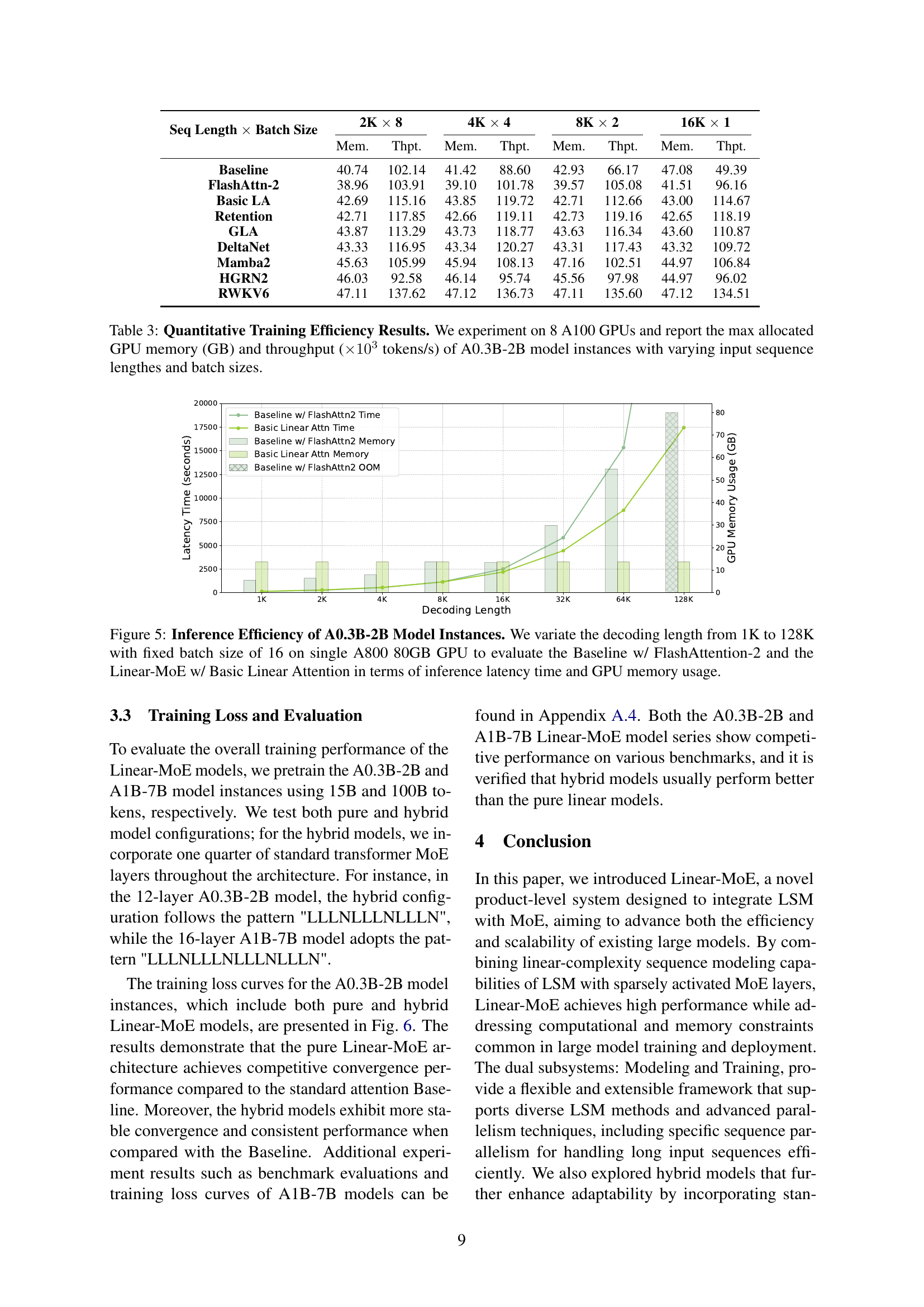
🔼 This table presents a quantitative analysis of the training efficiency of different Linear-MoE model instances (A0.3B-2B) using eight A100 GPUs. It compares various LSM methods (Basic Linear Attention, FlashAttention-2, Retention, GLA, DeltaNet, Mamba2, HGRN2, RWKV6) across different input sequence lengths (2K, 4K, 8K, 16K) and corresponding batch sizes. For each configuration, the table reports the maximum allocated GPU memory (in GB) and the training throughput (in thousands of tokens per second). This data allows for a comprehensive evaluation of the memory usage and speed performance of each LSM method under varying sequence lengths and batch sizes.
read the caption
Table 3: Quantitative Training Efficiency Results. We experiment on 8 A100 GPUs and report the max allocated GPU memory (GB) and throughput (×103absentsuperscript103\times 10^{3}× 10 start_POSTSUPERSCRIPT 3 end_POSTSUPERSCRIPT tokens/s) of A0.3B-2B model instances with varying input sequence lengthes and batch sizes.
| MoE Optimization | Memory (GB) | Time/Iter (ms) |
| Baseline | 35.28 | 1565.6 |
| Grouped GEMM | 35.01 | 455.4 |
| MegaBlocks | 36.90 | 348.8 |
🔼 This table presents a performance comparison of different training configurations for the A0.3B-2B Linear-MoE model. The ‘Above’ section shows the impact of MoE optimization techniques (Grouped GEMM and MegaBlocks) on training efficiency, measured by memory usage per GPU and time per iteration. The ‘Below’ section demonstrates the effect of various parallelism strategies (Tensor, Pipeline, and Expert Parallelism) on training efficiency. The experiments were conducted on a single node with 8 A100 GPUs, using a sequence length of 2048 and a batch size of 4. The Baseline represents a standard Megatron-Core MoE implementation without any optimizations.
read the caption
Table 4: Above: MoE Optimization. Below: Distributed training efficiency under different parallelism settings. We report the memory usage per GPU (GB) and elapsed time per iteration (ms) while training the A0.3B-2B model with a sequence length of 2048 and a batch size of 4, using a node equipped with 8 A100 GPUs. The Baseline refers to the MoE implementation in Megatron-Core, which is used without any optimizations.
| EP | TP | PP | Memory (GB) | Time/Iter (ms) |
| 1 | 1 | 1 | 35.28 | 1565.6 |
| 8 | 1 | 1 | 22.98 | 739.4 |
| 1 | 8 | 1 | 10.04 | 6879.0 |
| 1 | 1 | 8 | 8.89 | 1820.2 |
| 2 | 2 | 2 | 12.90 | 1684.9 |
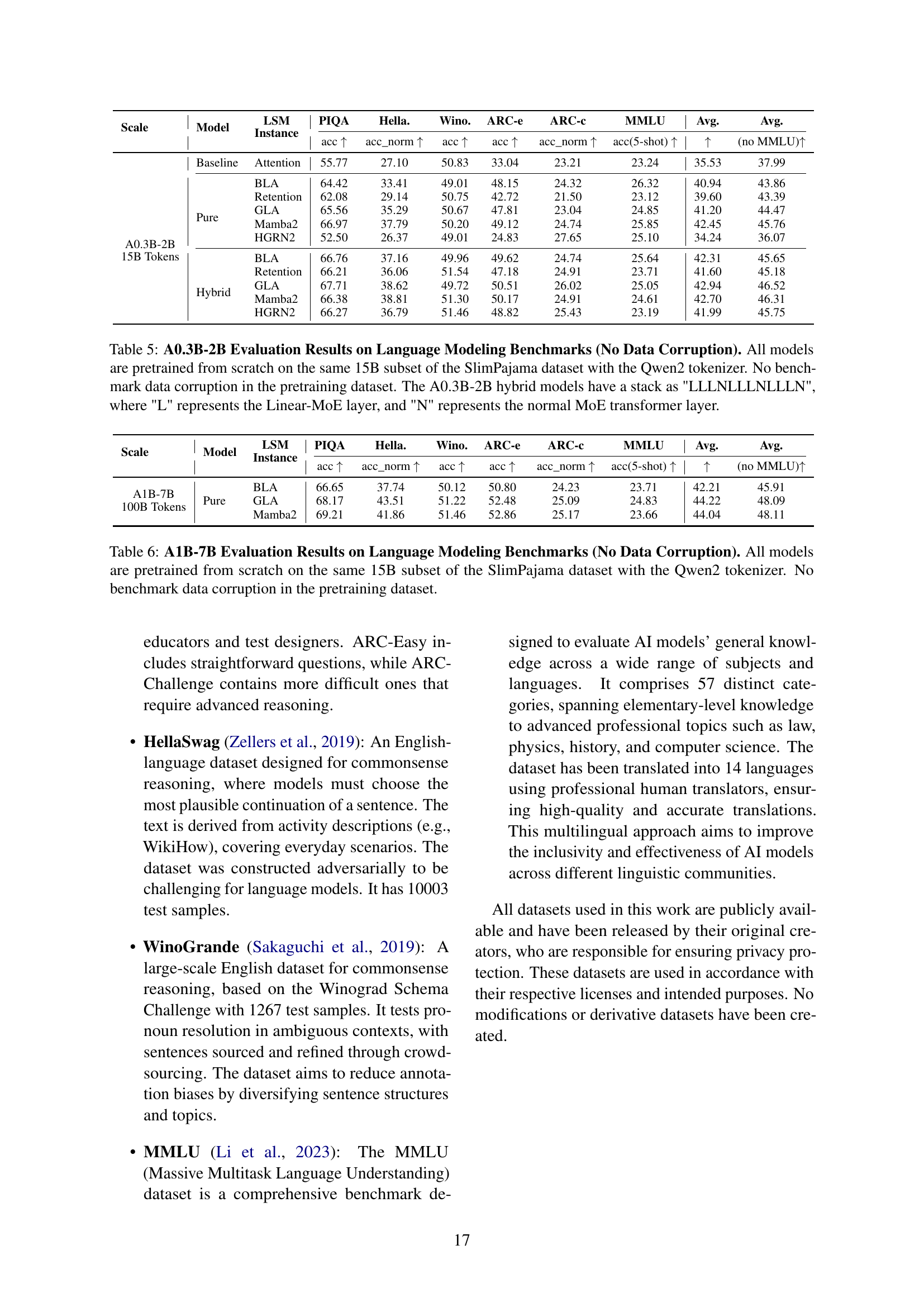
🔼 Table 5 presents the evaluation results of A0.3B-2B Linear-MoE models on various language modeling benchmarks. The models were all trained from scratch using the same 15B tokens from the SlimPajama dataset and the Qwen2 tokenizer. Crucially, no data corruption was introduced during pretraining. The table compares the performance of several different LSM (Linear Sequence Modeling) methods—basic linear attention (BLA), Retention, GLA, Mamba2, and HGRN2—both in pure Linear-MoE models (all Linear-MoE layers) and hybrid Linear-MoE models (a mix of Linear-MoE and standard transformer MoE layers, with the hybrid model architecture following a specific ‘LLLNLLLNLLLN’ pattern). The benchmarks include PIQA, HellaSwag, Winogrande, ARC-Easy, ARC-Challenge, and MMLU.
read the caption
Table 5: A0.3B-2B Evaluation Results on Language Modeling Benchmarks (No Data Corruption). All models are pretrained from scratch on the same 15B subset of the SlimPajama dataset with the Qwen2 tokenizer. No benchmark data corruption in the pretraining dataset. The A0.3B-2B hybrid models have a stack as 'LLLNLLLNLLLN', where 'L' represents the Linear-MoE layer, and 'N' represents the normal MoE transformer layer.
| Scale | Model | LSM Instance | PIQA | Hella. | Wino. | ARC-e | ARC-c | MMLU | Avg. | Avg. |
| acc | acc_norm | acc | acc | acc_norm | acc(5-shot) | (no MMLU) | ||||
| Baseline | Attention | 55.77 | 27.10 | 50.83 | 33.04 | 23.21 | 23.24 | 35.53 | 37.99 | |
| A0.3B-2B 15B Tokens | Pure | BLA | 64.42 | 33.41 | 49.01 | 48.15 | 24.32 | 26.32 | 40.94 | 43.86 |
| Retention | 62.08 | 29.14 | 50.75 | 42.72 | 21.50 | 23.12 | 39.60 | 43.39 | ||
| GLA | 65.56 | 35.29 | 50.67 | 47.81 | 23.04 | 24.85 | 41.20 | 44.47 | ||
| Mamba2 | 66.97 | 37.79 | 50.20 | 49.12 | 24.74 | 25.85 | 42.45 | 45.76 | ||
| HGRN2 | 52.50 | 26.37 | 49.01 | 24.83 | 27.65 | 25.10 | 34.24 | 36.07 | ||
| Hybrid | BLA | 66.76 | 37.16 | 49.96 | 49.62 | 24.74 | 25.64 | 42.31 | 45.65 | |
| Retention | 66.21 | 36.06 | 51.54 | 47.18 | 24.91 | 23.71 | 41.60 | 45.18 | ||
| GLA | 67.71 | 38.62 | 49.72 | 50.51 | 26.02 | 25.05 | 42.94 | 46.52 | ||
| Mamba2 | 66.38 | 38.81 | 51.30 | 50.17 | 24.91 | 24.61 | 42.70 | 46.31 | ||
| HGRN2 | 66.27 | 36.79 | 51.46 | 48.82 | 25.43 | 23.19 | 41.99 | 45.75 |
🔼 This table presents the evaluation results for the A1B-7B model series on various language modeling benchmarks. The A1B-7B models, each with 7 billion parameters and 1 billion activated parameters, were trained from scratch using a 15-billion token subset of the SlimPajama dataset and the Qwen2 tokenizer. The results are categorized by the type of Linear Sequence Modeling (LSM) method used (BLA, GLA, Mamba2), whether the model was a pure Linear-MoE model or a hybrid model (combining Linear-MoE and standard Transformer layers), and include metrics like accuracy and accuracy normalized for benchmarks including PIQA, HellaSwag, Winograd Schema Challenge, ARC-Easy, ARC-Challenge, and MMLU. Crucially, no data corruption was introduced during the pretraining phase.
read the caption
Table 6: A1B-7B Evaluation Results on Language Modeling Benchmarks (No Data Corruption). All models are pretrained from scratch on the same 15B subset of the SlimPajama dataset with the Qwen2 tokenizer. No benchmark data corruption in the pretraining dataset.
Full paper#