TL;DR#
Autonomous driving relies on generating high-quality, multimodal trajectories, but current methods struggle with trajectory selection and inconsistencies between guidance and scene information. This leads to complexity and reduced trajectory quality, hindering the development of robust end-to-end systems. Recent diffusion-based approaches, while promising, often suffer from trajectory divergence, requiring complex scoring mechanisms and HD maps, which are difficult to obtain in all environments. These limitations underscore the need for improved methods that can effectively constrain trajectory generation and enhance overall system reliability.
The paper introduces GoalFlow, a novel method that effectively constrains the generative process using goal-driven flow matching. GoalFlow consists of perception module, goal point construction module, and trajectory planning module. This approach uses a scoring mechanism to select the best goal point from candidate points, based on scene information, and employs flow matching for efficient multimodal trajectory generation. Experimental results on the Navsim dataset demonstrate that GoalFlow achieves state-of-the-art performance, delivering robust multimodal trajectories. It is significantly surpassing existing methods, while requiring only a single denoising step for excellent performance.
Key Takeaways#
Why does it matter?#
GoalFlow offers a robust method for multimodal trajectory generation, outperforming existing techniques in critical safety metrics and opening new research directions for generative models in autonomous driving. It advances end-to-end autonomous driving systems towards safer and more reliable navigation.
Visual Insights#

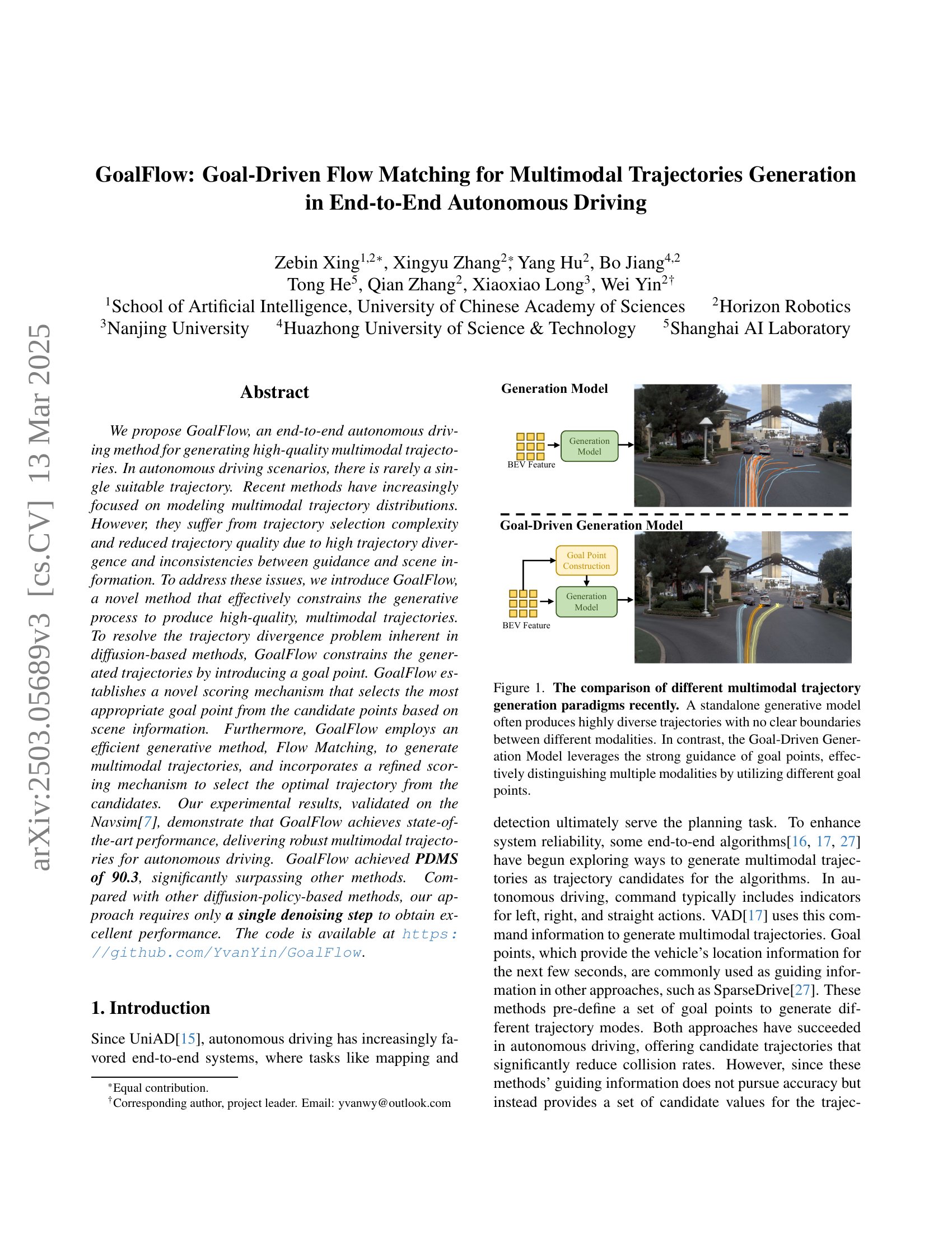
🔼 This figure compares different approaches to multimodal trajectory generation in autonomous driving. A standalone generative model is shown to produce a wide range of trajectories that blend together without clear distinctions between different driving behaviors (e.g., turning left vs. going straight). In contrast, the ‘Goal-Driven Generation Model’ uses goal points to guide the trajectory generation process, resulting in distinct trajectory clusters, each corresponding to a different driving maneuver. The use of goal points effectively separates the different trajectory modalities, leading to improved clarity and quality of the generated paths.
read the caption
Figure 1: The comparison of different multimodal trajectory generation paradigms recently. A standalone generative model often produces highly diverse trajectories with no clear boundaries between different modalities. In contrast, the Goal-Driven Generation Model leverages the strong guidance of goal points, effectively distinguishing multiple modalities by utilizing different goal points.
| Method | Ego Stat. | Image | LiDAR | Video | ||||||
| Constant Velocity | ✓ | 68.0 | 57.8 | 50.0 | 100 | 19.4 | 20.6 | |||
| Ego Status MLP | ✓ | 93.0 | 77.3 | 83.6 | 100 | 62.8 | 65.6 | |||
| LTF [3] | ✓ | ✓ | 97.4 | 92.8 | 92.4 | 100 | 79.0 | 83.8 | ||
| TransFuser [3] | ✓ | ✓ | ✓ | 97.7 | 92.8 | 92.8 | 100 | 79.2 | 84.0 | |
| UniAD [15] | ✓ | ✓ | ✓ | 97.8 | 91.9 | 92.9 | 100 | 78.8 | 83.4 | |
| PARA-Drive [30] | ✓ | ✓ | ✓ | ✓ | 97.9 | 92.4 | 93.0 | 99.8 | 79.3 | 84.0 |
| GoalFlow (Ours) | ✓ | ✓ | ✓ | 98.4 | 98.3 | 94.6 | 100 | 85.0 | 90.3 | |
| ✓ | ✓ | ✓ | 99.8 | 97.9 | 98.6 | 100 | 85.4 | 92.1 | ||
| 100 | 100 | 100 | 99.9 | 87.5 | 94.8 |
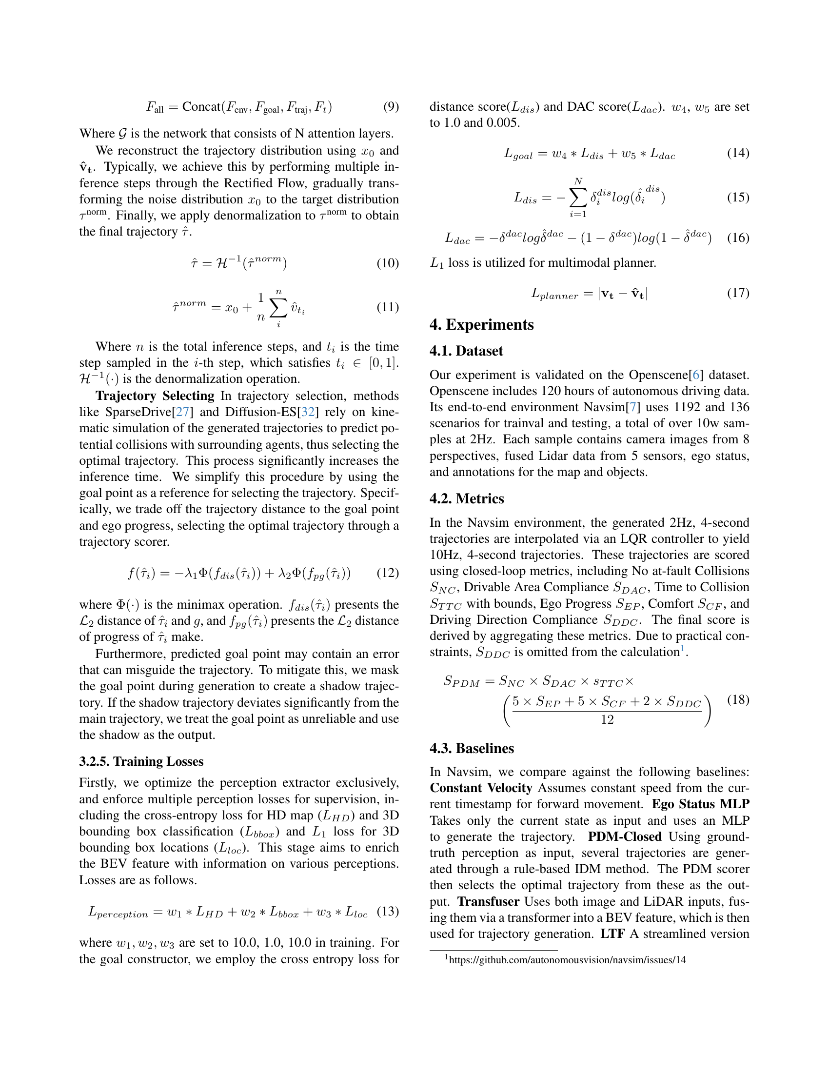
🔼 Table 1 presents a comparison of the proposed GoalFlow model with state-of-the-art (SOTA) methods for autonomous driving trajectory generation, evaluated using the PDM (Predictive Driving Metrics) score on the Navsim dataset. The table shows that GoalFlow outperforms all other methods across all key metrics (SNC, SDAC, STTC, SCF, SEP, and SPDM). Two additional rows highlight results using either the endpoint of the ground truth trajectory or the ground truth trajectories themselves for evaluation, further illustrating GoalFlow’s performance.
read the caption
Table 1: Comparisons with SOTA methods in PDM score metrics on Navsim [7] Test. Our method outperforms other approaches across all evaluation metrics. ††{\dagger}† uses the endpoint of the ground-truth trajectory as the goal point. ‡‡{\ddagger}‡ uses the ground-truth trajectories to evaluate.
In-depth insights#
GoalFlow: Overview#
GoalFlow’s overview likely details its core architecture and functionality, acting as a high-level introduction to the method. It probably articulates the key components and how they interact to achieve the primary goal: generating high-quality, multimodal trajectories for autonomous driving. The overview would highlight how GoalFlow addresses limitations in existing approaches, such as trajectory divergence and inconsistencies between guidance and scene information. It would likely emphasize the importance of the goal-driven approach, explaining how carefully constructed goal points constrain the generative process. Also it touches on the perception module for feature extraction from image and LiDAR data, goal point construction module to select the most suitable goal point and trajectory generation module using Flow Matching. The overview likely emphasizes that GoalFlow consists of three modules: perception module for BEV feature extraction, goal point construction module to select the optimal goal point for guidance and finally trajectory planning module to generate trajectories by denoising from the Gaussian distribution to the target distribution. The overview will likely summarize the benefits achieved by GoalFlow, such as state-of-the-art performance and reduced computational complexity.
Goal-Driven FM#
Goal-Driven Flow Matching (FM) likely focuses on leveraging flow matching techniques, which excel at mapping probability distributions, guided by specific goals. In autonomous driving, this means generating trajectories that are not just diverse but also intentionally directed towards pre-defined goal states. This approach contrasts with unguided generative models that might produce trajectories lacking clear objectives. A key challenge involves effectively defining and representing these goals in a way that is compatible with the FM framework. This could involve using goal points, which represent desired future locations or states of the vehicle. By conditioning the flow matching process on these goals, the generated trajectories are more likely to be relevant and useful for planning. The effectiveness of Goal-Driven FM hinges on the accuracy and relevance of the goal representation, as well as the ability of the FM model to seamlessly integrate this information into the trajectory generation process.
Navsim Validation#
Although the exact phrase “Navsim Validation” isn’t explicitly present, the paper validates its approach through experiments conducted within the Navsim environment, a crucial aspect for assessing autonomous driving algorithms. The choice of Navsim suggests a controlled, simulated setting allowing for repeatable testing and precise measurement of performance metrics. The validation likely focuses on evaluating the generated trajectories using closed-loop metrics like collision avoidance, drivable area compliance, and progress. Analyzing performance within Navsim provides insights into the algorithm’s robustness and safety before real-world deployment. The paper would detail how GoalFlow’s performance on Navsim compares to baseline methods, emphasizing improvements in key metrics related to safe and efficient navigation. The validation likely investigates the impact of GoalFlow’s components and parameters on trajectory quality and multimodal capabilities within the simulated environment. The results from the Navsim validation are vital for demonstrating the effectiveness and promise of the GoalFlow framework for autonomous driving applications. Also the Metrics used in Navsim can be a good way to determine the performance of the model.
Single-step Robust#
The concept of “single-step robust” likely refers to a method’s ability to maintain performance or stability when subjected to a single, significant perturbation or outlier data point. In machine learning, this is valuable because real-world datasets often contain noisy or erroneous data. A model that is single-step robust would not drastically change its predictions or internal parameters due to one bad sample. This could be achieved through various techniques such as robust loss functions (e.g., Huber loss) that are less sensitive to outliers, data preprocessing steps to identify and mitigate outliers, or regularization methods that prevent the model from overfitting to single data points. The term highlights a practical focus on immediate resilience to isolated errors, rather than aggregate performance over a distribution of noisy data. Further, in end-to-end systems, the single denoising step also means single-step robust
Beyond Diversity#
While diversity aims to include a range of perspectives, it can sometimes fall short of fostering true collaboration and understanding. Going beyond diversity means actively cultivating inclusion, where every voice is not only heard but also valued and integrated into decision-making processes. This requires creating a culture of equity, ensuring that everyone has equal opportunities to contribute and succeed, regardless of their background or identity. Furthermore, it necessitates addressing systemic biases and power imbalances that may hinder full participation. A truly impactful approach moves beyond mere representation to focus on creating a sense of belonging for all individuals, promoting empathy, and celebrating the richness that diverse perspectives bring to innovation and problem-solving. It’s about building bridges and fostering a shared commitment to creating a more just and equitable environment. This is a continuous journey that demands ongoing reflection, learning, and action.
More visual insights#
More on figures

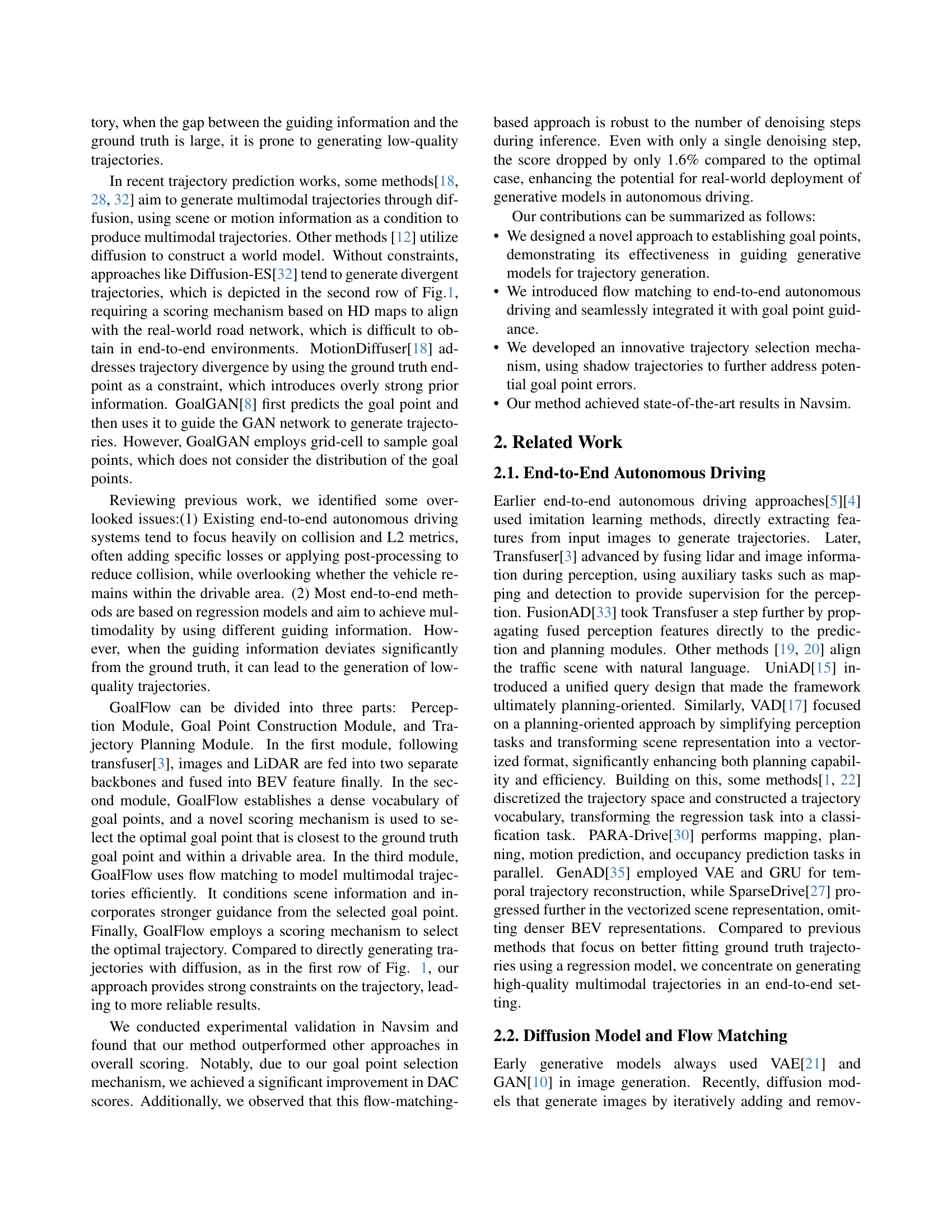
🔼 GoalFlow’s architecture is composed of three modules: the Perception Module, the Goal Point Construction Module, and the Trajectory Planning Module. The Perception Module takes image and LiDAR data as input, processing them to generate a Bird’s Eye View (BEV) feature representation, denoted as Fbev. This BEV feature is then passed to the Goal Point Construction Module. This module utilizes a Goal Point Vocabulary (a set of potential goal points) to identify the optimal goal point for trajectory generation, using a scoring mechanism. The selected goal point is then given to the Trajectory Planning Module, which uses a denoising process to generate multiple trajectory candidates starting from a Gaussian distribution and converging towards the target distribution. These candidates are then evaluated by a Trajectory Scorer, which selects the single best trajectory.
read the caption
Figure 2: Overview of the GoalFlow architecture. GoalFlow consists of three modules. The Perception Module is responsible for integrating scene information into a BEV feature Fbevsubscript𝐹𝑏𝑒𝑣F_{bev}italic_F start_POSTSUBSCRIPT italic_b italic_e italic_v end_POSTSUBSCRIPT, the Goal Point Construction Module selects the optimal goal point from Goal Point Vocabulary 𝕍𝕍\mathbb{V}blackboard_V as guidance information, and the Trajectory Planning Module generates the trajectories by denoising from the Gaussian distribution to the target distribution. Finally, the Trajectory Scorer selects the optimal trajectory from the candidates.

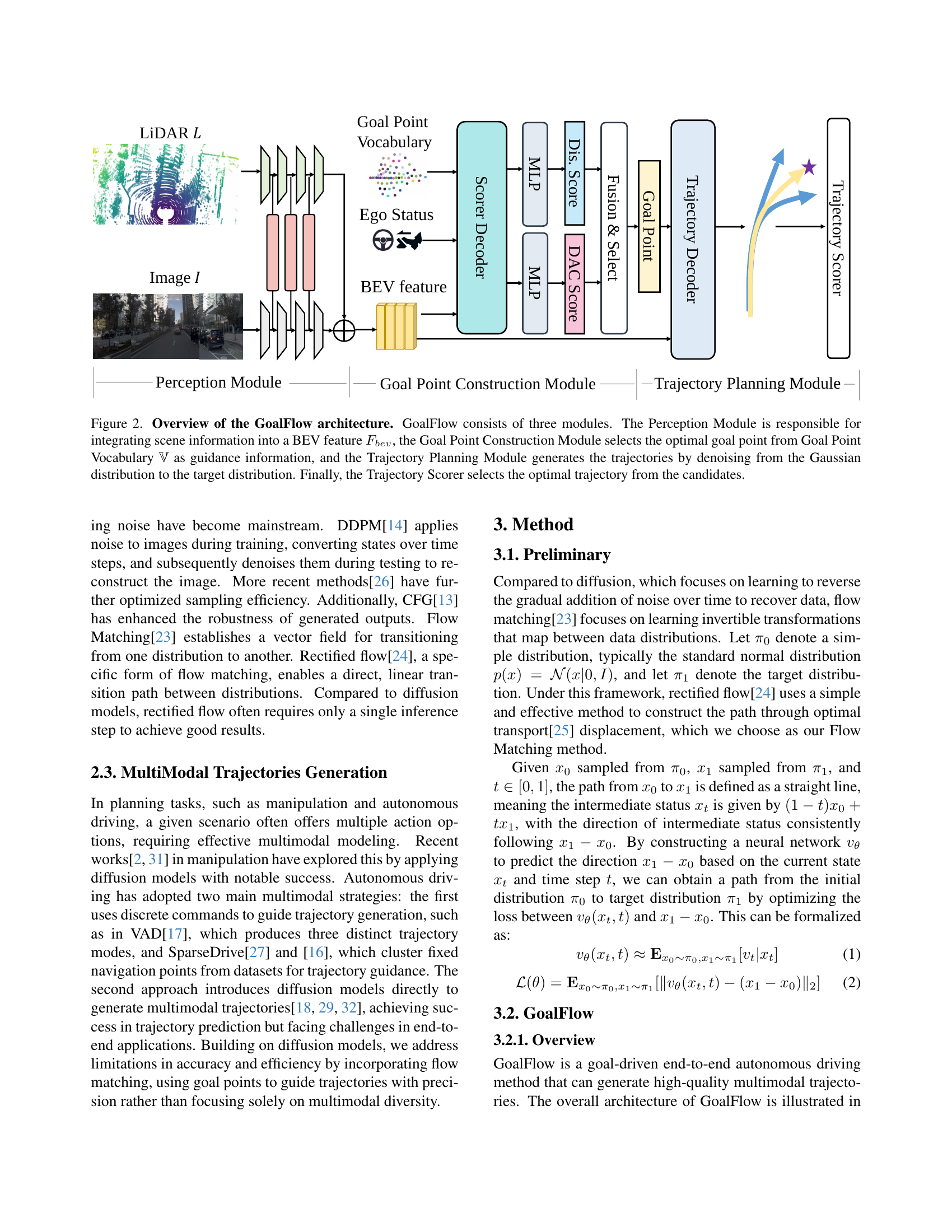
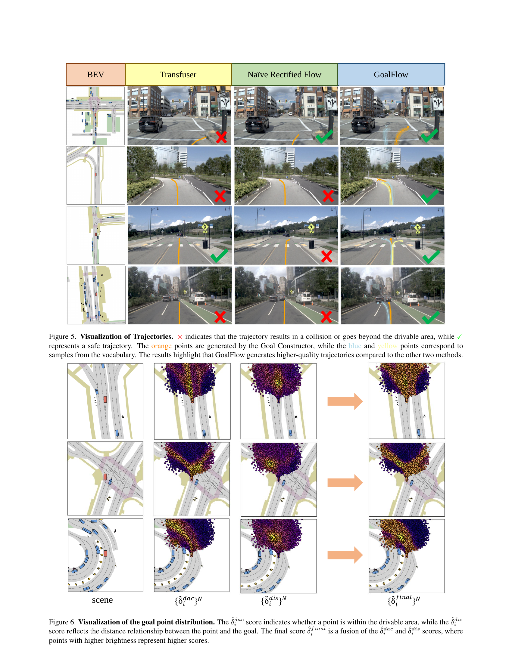
🔼 This figure shows the detailed structure of the Goal Point Construction Module. It visually depicts how the module processes the BEV feature (Fbev), ego status (Fego), and the goal point vocabulary (V) to select the optimal goal point. The figure highlights the key components: the vocabulary encoder, the scorer decoder (using MLPs), and the final goal point selection process. The accompanying text (b) illustrates the distributions of distance score (dis), drivable area compliance score (dac), and final score (final). Warmer colors indicate higher scores.
read the caption
(a)

🔼 This figure shows the score distributions of the Distance Score (dis), Drivable Area Compliance Score (dac), and the final score (ffinal) for goal point selection. Warmer colors indicate higher scores. The Distance Score measures how close a goal point is to the ground truth. The Drivable Area Compliance Score checks if the goal point is within a drivable area. The final score combines both scores to select the best goal point.
read the caption
(b)

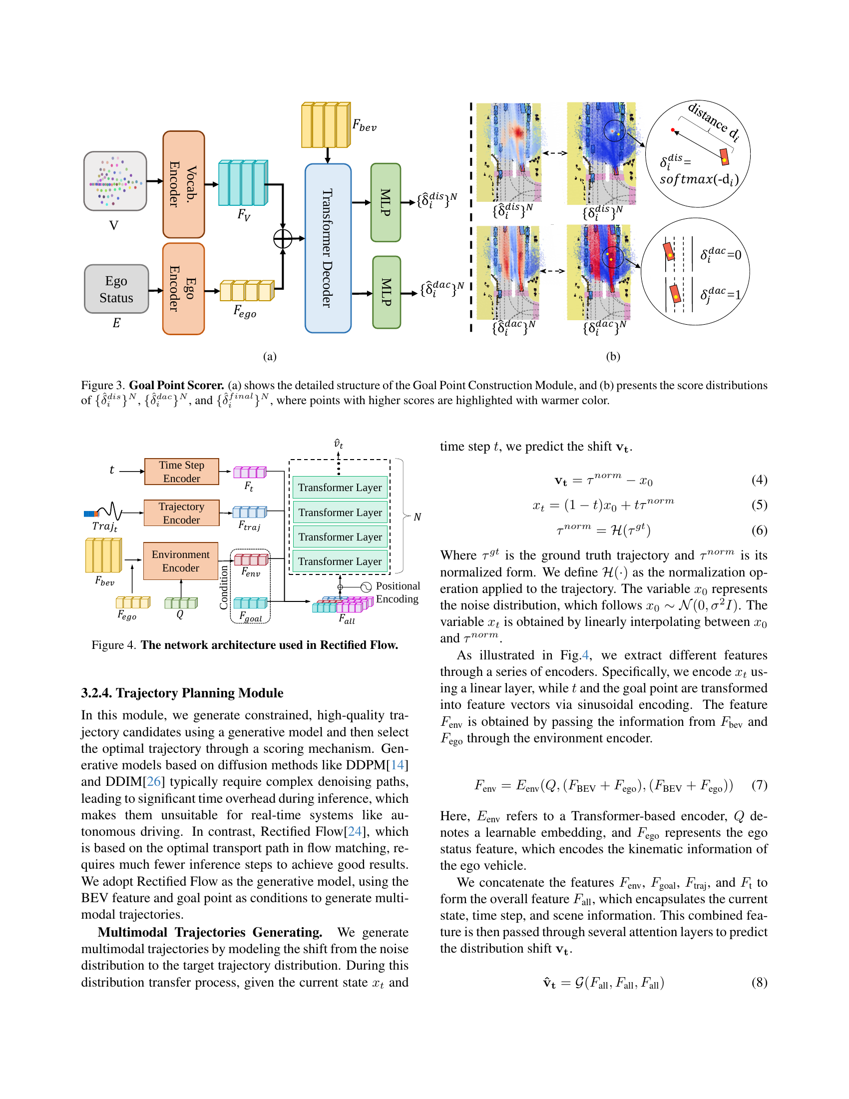
🔼 Figure 3 illustrates the Goal Point Construction Module, a key component of the GoalFlow architecture. Part (a) provides a detailed diagram of this module’s structure, showing how it uses a transformer-based scorer decoder to generate distance and drivable area compliance scores for each potential goal point. Part (b) visualizes the resulting score distributions (distance score, drivable area compliance score, and final score), using a color gradient to represent the magnitude of each score—warmer colors indicating higher scores. This visualization helps to understand how the module effectively selects the most appropriate goal point for trajectory generation.
read the caption
Figure 3: Goal Point Scorer. (a) shows the detailed structure of the Goal Point Construction Module, and (b) presents the score distributions of {δ^idis}Nsuperscriptsubscriptsuperscript^𝛿𝑑𝑖𝑠𝑖𝑁\{\hat{\delta}^{dis}_{i}\}^{N}{ over^ start_ARG italic_δ end_ARG start_POSTSUPERSCRIPT italic_d italic_i italic_s end_POSTSUPERSCRIPT start_POSTSUBSCRIPT italic_i end_POSTSUBSCRIPT } start_POSTSUPERSCRIPT italic_N end_POSTSUPERSCRIPT, {δ^idac}Nsuperscriptsubscriptsuperscript^𝛿𝑑𝑎𝑐𝑖𝑁\{\hat{\delta}^{dac}_{i}\}^{N}{ over^ start_ARG italic_δ end_ARG start_POSTSUPERSCRIPT italic_d italic_a italic_c end_POSTSUPERSCRIPT start_POSTSUBSCRIPT italic_i end_POSTSUBSCRIPT } start_POSTSUPERSCRIPT italic_N end_POSTSUPERSCRIPT, and {δ^ifinal}Nsuperscriptsubscriptsuperscript^𝛿𝑓𝑖𝑛𝑎𝑙𝑖𝑁\{\hat{\delta}^{final}_{i}\}^{N}{ over^ start_ARG italic_δ end_ARG start_POSTSUPERSCRIPT italic_f italic_i italic_n italic_a italic_l end_POSTSUPERSCRIPT start_POSTSUBSCRIPT italic_i end_POSTSUBSCRIPT } start_POSTSUPERSCRIPT italic_N end_POSTSUPERSCRIPT, where points with higher scores are highlighted with warmer color.

🔼 This figure illustrates the architecture of the Rectified Flow model employed in GoalFlow for trajectory generation. It shows how the model takes different inputs including time step (t), the current state (xt), and features from the environment (Fenv) and ego vehicle (Fego) to generate a trajectory. These features are processed through various encoder and transformer layers to produce a shift vector (vt), used for transitioning the trajectory from a noise distribution to a target distribution. The various components such as the encoder, transformer layers, and positional encoding are clearly depicted to show the process of trajectory prediction using the rectified flow framework.
read the caption
Figure 4: The network architecture used in Rectified Flow.
More on tables
| Model | Description | ||||||
|---|---|---|---|---|---|---|---|
| Transfuser[3] | 97.7 | 92.8 | 92.8 | 100 | 79.0 | 84.0 | |
| Base Model | 97.9 | 94.2 | 94.2 | 100 | 79.9 | 85.6 | |
| + Distance Score Map | 98.5 | 96.4 | 94.9 | 100 | 83.0 | 88.5 | |
| + DAC Score Map | 98.6 | 97.5 | 94.7 | 100 | 83.8 | 89.4 | |
| + Trajectory Scorer | 98.4 | 98.3 | 94.6 | 100 | 85.0 | 90.3 |
🔼 This table presents an ablation study analyzing the impact of different components on the model’s performance. The base model (ℳ₀) uses rectified flow without goal point guidance, averaging all generated trajectories for the final output. Adding the distance score map (ℳ₁) improves the model by providing distance information for guidance. Further enhancement comes from incorporating the drivable area compliance (DAC) score map (ℳ₂), which adds constraints to keep trajectories within drivable areas. Finally, adding a trajectory scorer (ℳ₃) refines the selection process for the optimal trajectory among the candidates.
read the caption
Table 2: Ablation study on the influence of each component. ℳ0subscriptℳ0\mathcal{M}_{0}caligraphic_M start_POSTSUBSCRIPT 0 end_POSTSUBSCRIPT is the base model, which uses rectified flow without goal point guidance and averages all generated trajectories to produce the final output. ℳ1subscriptℳ1\mathcal{M}_{1}caligraphic_M start_POSTSUBSCRIPT 1 end_POSTSUBSCRIPT and ℳ2subscriptℳ2\mathcal{M}_{2}caligraphic_M start_POSTSUBSCRIPT 2 end_POSTSUBSCRIPT introduce the distance score map and DAC score map, respectively, to guide the rectified flow. ℳ3subscriptℳ3\mathcal{M}_{3}caligraphic_M start_POSTSUBSCRIPT 3 end_POSTSUBSCRIPT builds upon ℳ1subscriptℳ1\mathcal{M}_{1}caligraphic_M start_POSTSUBSCRIPT 1 end_POSTSUBSCRIPT by incorporating trajectory scorer.
| 20 | 177.8ms | 98.3 | 98.1 | 94.3 | 100 | 84.7 | 89.9 |
| 10 | 92.4ms | 98.3 | 98.2 | 94.4 | 100 | 84.9 | 90.1 |
| 5 | 49.0ms | 98.4 | 98.3 | 94.6 | 100 | 84.4 | 90.3 |
| 1 | 10.4ms | 98.4 | 97.8 | 94.1 | 100 | 84.5 | 88.9 |
🔼 This table presents an ablation study on the impact of varying the number of denoising steps (T) during inference on the performance of the GoalFlow model. It shows that the model’s performance metrics (SNC, SDAC, STTC, SCF, SEP, and SPDM) remain relatively stable across a wide range of denoising steps from 20 to 1, demonstrating the model’s robustness to this hyperparameter. This is a key finding, highlighting the efficiency of GoalFlow, as it requires only a few denoising steps to achieve excellent results. The inference time is also shown, demonstrating the significant reduction in computation time as the number of steps decreases.
read the caption
Table 3: Impact of different timesteps in inference. T𝑇Titalic_T denotes the number of denoising steps during inference. The results indicate that the model’s performance is robust to variations of denoising steps.
| 0.05 | 98.3 | 98.2 | 94.4 | 100 | 85.0 | 90.1 |
| 0.1 | 98.4 | 98.3 | 94.6 | 100 | 85.0 | 90.3 |
| 0.2 | 87.4 | 76.0 | 69.4 | 32.0 | 56.2 | 49.0 |
| 0.3 | 68.3 | 48.1 | 44.8 | 2.23 | 23.6 | 18.8 |
🔼 This table presents an ablation study analyzing the effect of varying the standard deviation (σ) of the initial noise distribution (x₀) on the performance of the GoalFlow model. The standard deviation (σ) controls the amount of noise added to the initial state of the trajectory generation process. The results demonstrate that model performance is relatively robust to changes in σ when σ is below 0.1. However, as σ increases beyond 0.1, the performance drops significantly, indicating that too much initial noise negatively impacts the model’s ability to generate high-quality trajectories.
read the caption
Table 4: Impact of different values of σ𝜎\sigmaitalic_σ on the initial noise distribution. σ𝜎\sigmaitalic_σ is the standard deviation of x0subscript𝑥0x_{0}italic_x start_POSTSUBSCRIPT 0 end_POSTSUBSCRIPT. The results show that performance drops significantly when σ𝜎\sigmaitalic_σ exceeds 0.1, but remains stable for values below 0.1.
| Dim | Backbone | |||||
|---|---|---|---|---|---|---|
| 256 | V2-99 | 97.1 | 96.2 | 91.8 | 81.8 | 86.5 |
| 512 | V2-99 | 97.3 | 97.6 | 92.5 | 83.0 | 88.1 |
| 1024 | V2-99 | 98.6 | 97.5 | 94.7 | 85.0 | 89.4 |
| 256 | resnet34 | 98.3 | 93.8 | 94.3 | 79.8 | 85.7 |
| 256 | V2-99 | 97.1 | 96.2 | 91.8 | 81.8 | 86.5 |
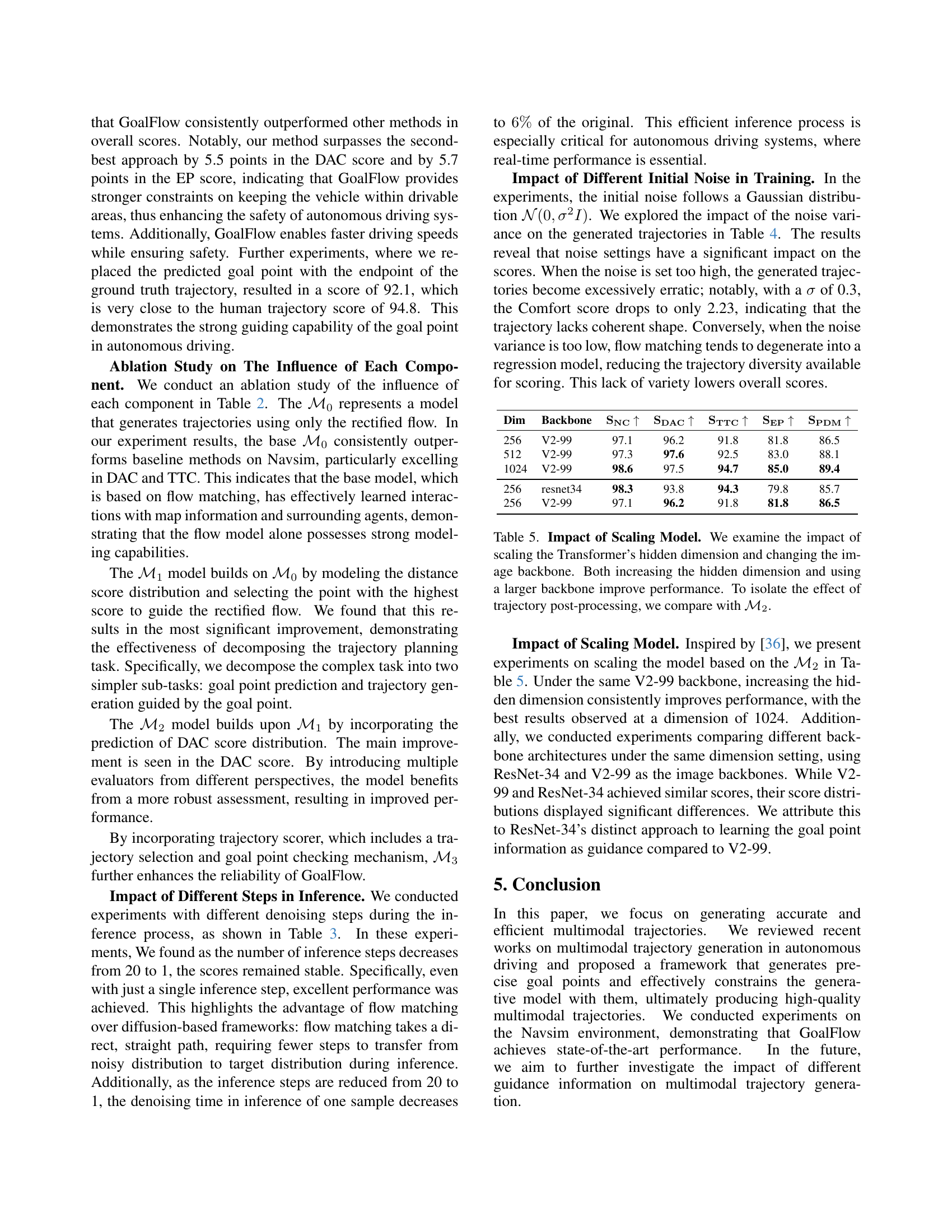
🔼 This table presents an ablation study on the impact of scaling the transformer’s hidden dimension and changing the image backbone in the GoalFlow model. The results show that increasing the hidden dimension and using a larger backbone (V2-99 vs. ResNet-34) generally lead to performance improvements, as measured by various metrics like SNC, SDAC, STTC, SEP, and SPDM. The table isolates the effect of trajectory post-processing by comparing results to the performance of model M2, which includes all other components except the changes made for this experiment.
read the caption
Table 5: Impact of Scaling Model. We examine the impact of scaling the Transformer’s hidden dimension and changing the image backbone. Both increasing the hidden dimension and using a larger backbone improve performance. To isolate the effect of trajectory post-processing, we compare with ℳ2subscriptℳ2\mathcal{M}_{2}caligraphic_M start_POSTSUBSCRIPT 2 end_POSTSUBSCRIPT.
Full paper#