TL;DR#
Recent advances in LLMs show remarkable success in following instructions, but handling those with multiple constraints remains a challenge. Existing works evaluating the ability of LLMs follow a bottom-up approach, starting from curated verifiable constraints. To evaluate the abilities of LLMs to follow real-world instructions, this paper introduces a large-scale dataset of real user instructions under diverse conditions.
This paper introduces WILDIFEVAL, a dataset of 12K real user instructions. It analyzes different types of user tasks and constraints to provide an insight into real-world generation use cases. The paper compares the performance of various LLMs and analyzes the impact of the number and type of constraints on model performance. Releasing WILDIFEVAL provides the first comprehensive analysis of the types and properties of constraints appearing in real-world user instructions.
Key Takeaways#
Why does it matter?#
This paper introduces WILDIFEVAL, a unique dataset with 12K real user instructions under multi-constraint to benchmark the abilities of instruction-following LLMs. WILDIFEVAL, aims to reflect a realistic and contemporary view of constrained generation user requests, serves as a playground for fine-grained analysis of the strengths and weaknesses of models, drilling down beyond the task level into atomic user constraints, can help focus model improvement efforts.
Visual Insights#

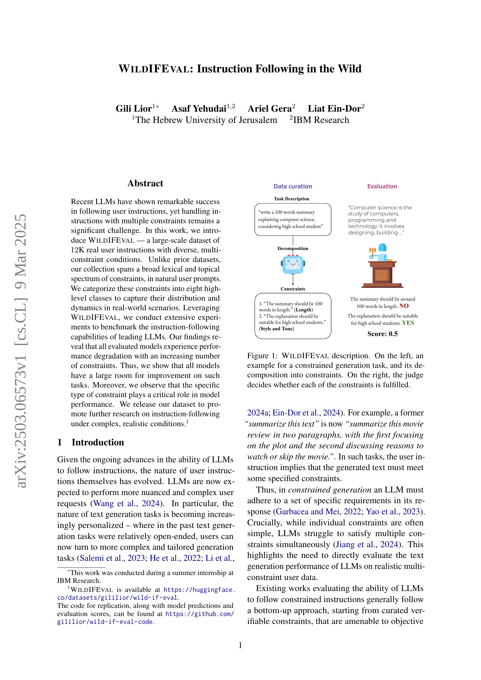
🔼 This figure illustrates the WILDIFEVAL dataset’s structure. The left side shows a sample user instruction for a text generation task, broken down into its individual constraints (e.g., length, style). The right side depicts how a human judge assesses whether the generated text satisfies each constraint, ultimately determining the task’s overall score. This process reveals the challenges LLMs face in fulfilling multiple constraints simultaneously.
read the caption
Figure 1: WildIFEval description. On the left, an example for a constrained generation task, and its decomposition into constraints. On the right, the judge decides whether each of the constraints is fulfilled.
| Benchmark | Data Source | Evaluation | Size |
| IFEval | Synthetic | Rule | 541 |
| FollowBench | Crowd + Syn. | Model / Rule | 795 |
| InfoBench | Crowd | Model / Rule | 500 |
| WildIFEval (Ours) | Real Users | Model | 11,813 |
🔼 This table compares WildIFEval to three other publicly available instruction-following benchmarks: IFEval, FollowBench, and InfoBench. For each benchmark, it shows the data source used for creating the benchmark (e.g., synthetic data, crowd-sourced data, or real users), the evaluation method used (e.g., rule-based, model-based, or a combination), and the size of the benchmark (number of tasks). This allows for a comparison of the scale and methodology of different benchmarks, highlighting WildIFEval’s unique characteristics such as its use of real-world user instructions.
read the caption
Table 1: Comparison of WildIFEval with openly available instruction-following benchmarks such as IFEval Zhou et al. (2023), FollowBench Jiang et al. (2024), and InfoBench Qin et al. (2024).
In-depth insights#
Multi-Constraint#
Multi-constraint scenarios in research highlight the complexities of real-world problems. Balancing multiple objectives and limitations requires sophisticated approaches. Traditional methods often struggle, leading to suboptimal solutions. AI and optimization techniques offer promising tools for addressing these challenges. Effective strategies involve prioritization, trade-off analysis, and robustness evaluation. Future research should focus on scalable algorithms and adaptive constraint handling to improve decision-making.
Dataset: WILDIFE#
The WILDIFEVAL dataset is introduced as a large-scale resource for evaluating LLMs on multi-constraint instructions. Comprising 12K real-world user instructions, it aims to tackle the challenge of LLMs struggling with complex constraints. Unlike existing datasets, WILDIFEVAL captures a broad lexical and topical range of constraints found in natural user prompts, categorized into eight high-level classes. The dataset enables a fine-grained analysis of LLM performance, breaking down tasks into individual constraints for evaluation. Its release promotes research on instruction-following under complex, realistic conditions and fills a gap in realistic and diverse instructions.
Constraint Types#
Constraint types in generation tasks are diverse, ranging from explicit content rules (include/avoid) to nuanced stylistic and quality directives. Taxonomies often lack unification, needing bridging with data-driven insights. Analyzing frequent words helps uncover patterns and refine categories, revealing overlooked types. Persona/role and style/tone significantly shape the output’s narrative voice.
LLM Benchmarking#
LLM benchmarking is vital for assessing model capabilities. The paper uses WILDIFEVAL to evaluate LLMs, focusing on instruction-following in complex scenarios. The method measures the fraction of fulfilled constraints. The paper evaluates 14 LLMs. Results show that larger models generally perform better, but all models struggle with multiple constraints, especially those related to length. Specific constraint types influence model rankings.
Atomic Analysis#
Atomic analysis in the context of LLMs instruction following could refer to a granular, component-level investigation of model behavior. It entails breaking down complex instructions into individual constraints or sub-tasks and evaluating the model’s success in fulfilling each one. This allows for identifying specific strengths and weaknesses, pinpointing which types of constraints models handle well and where they struggle. By focusing on these atomic elements, researchers can gain deeper insights into the model’s decision-making process, leading to more targeted improvements in instruction following capabilities and a better understanding of the relationship between instruction components and model performance.
More visual insights#
More on figures

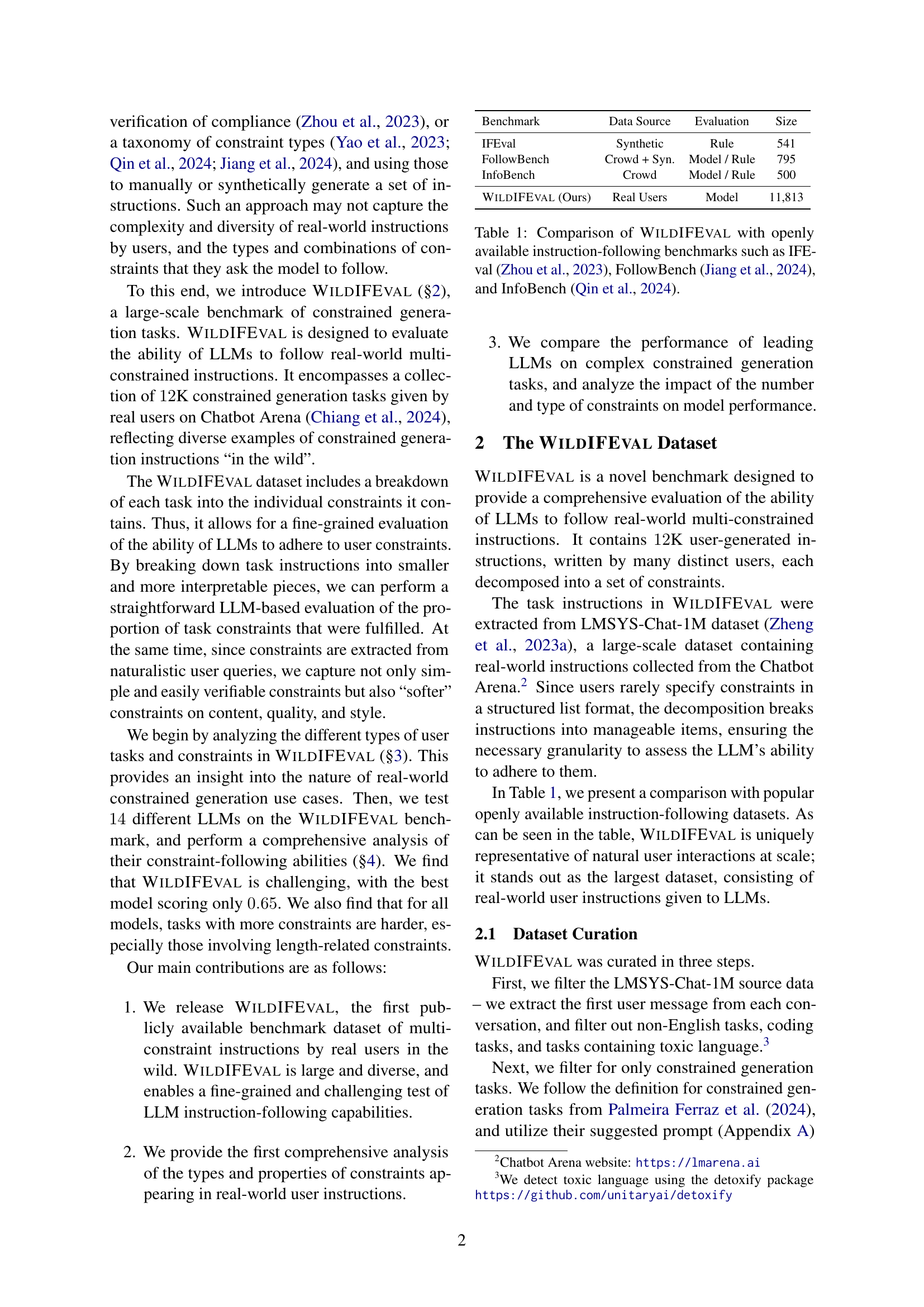
🔼 The figure shows the distribution of constraint types in the WILDIFEVAL dataset. It’s a bar chart visualizing the frequency of different constraint types, offering insights into the prevalence of various types of constraints in real-world user instructions. This helps understand the characteristics and complexity of user requests in terms of the types of constraints they impose on LLMs.
read the caption
(a)

🔼 This t-SNE projection of constraint embeddings shows clusters corresponding to certain constraint types, such as format and structure, length, and style and tone constraints, while others, like focus/emphasis and include/avoid, are more spread out.
read the caption
(b)

🔼 This figure displays the Kendall’s Tau correlation coefficients between the model rankings generated by different constraint types within the WILDIFEVAL benchmark. Values closer to 1 indicate stronger agreement in model rankings between the constraint types. This visualization helps to understand the relationship and potential overlap between various constraints, revealing whether models’ abilities to handle one type of constraint correlate with their abilities on other constraint types.
read the caption
(c)

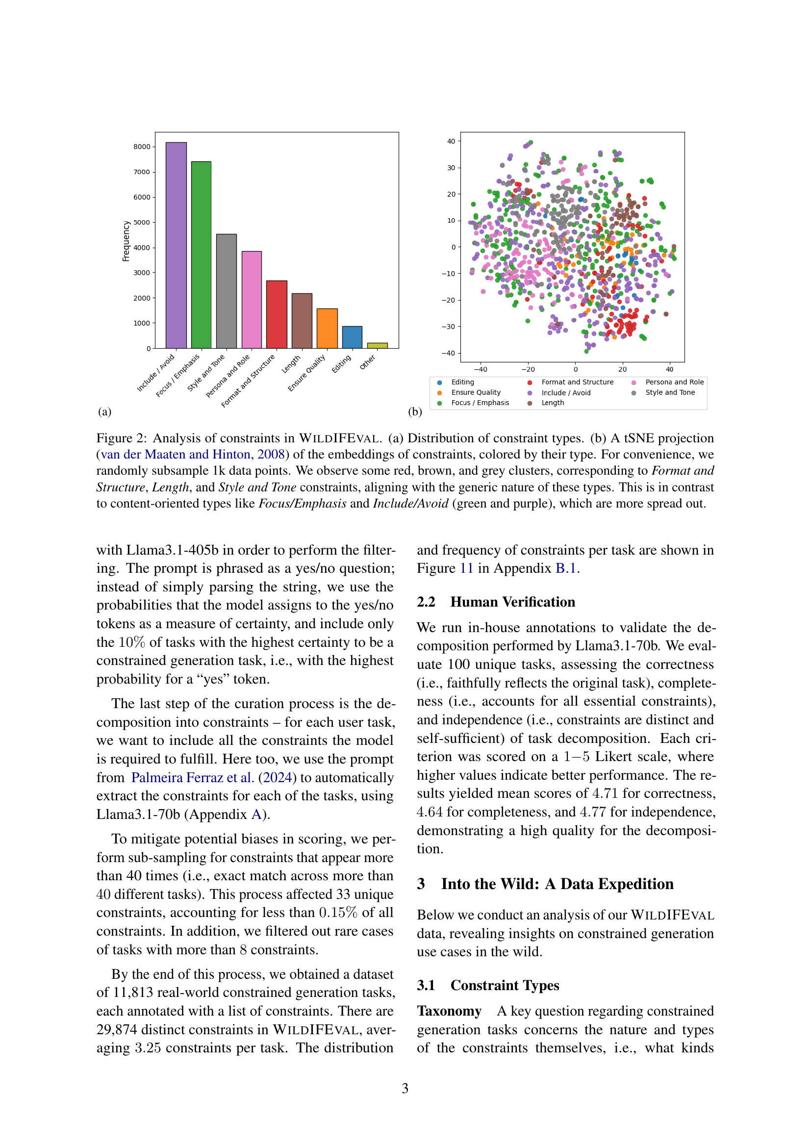
🔼 This figure shows the relative co-occurrence of constraint categories within tasks in the WILDIFEVAL dataset. It uses a heatmap to visualize how often pairs of constraint types appear together in the same task, compared to what would be expected based on their individual frequencies. Values above 1 indicate that constraints co-occur more frequently than expected by chance, suggesting potential relationships between constraint types. For example, a strong co-occurrence might indicate that certain types of constraints are often requested together by users.
read the caption
(d)

🔼 Figure 2 visualizes the analysis of constraints within the WildIFEval dataset. Panel (a) presents a bar chart illustrating the distribution of various constraint types, showing their relative frequencies. Panel (b) shows a t-distributed Stochastic Neighbor Embedding (t-SNE) projection of constraint embeddings, where each point represents a constraint and is colored according to its type. The t-SNE visualization reveals clustering patterns: constraints related to ‘Format and Structure’, ‘Length’, and ‘Style and Tone’ form distinct clusters, while ‘Focus/Emphasis’ and ‘Include/Avoid’ constraints are more dispersed. This suggests that the former group possesses a more inherent, generic nature than the latter content-oriented group.
read the caption
Figure 2: Analysis of constraints in WildIFEval. (a) Distribution of constraint types. (b) A tSNE projection van der Maaten and Hinton (2008) of the embeddings of constraints, colored by their type. For convenience, we randomly subsample 1k data points. We observe some red, brown, and grey clusters, corresponding to Format and Structure, Length, and Style and Tone constraints, aligning with the generic nature of these types. This is in contrast to content-oriented types like Focus/Emphasis and Include/Avoid (green and purple), which are more spread out.

🔼 This figure shows the relative co-occurrence of different constraint categories within the tasks in the WILDIFEVAL dataset. It compares the observed co-occurrence frequency of constraint pairs to what would be expected based on the individual frequencies of each constraint type. Values above 1 indicate that pairs of constraints appear together more frequently than expected by chance alone. The Appendix provides further details on the statistical calculations used.
read the caption
Figure 3: Relative co-occurrence of constraint categories within tasks. Values above 1111 indicate that constraints co-occur more than expected by their overall type frequencies. Refer to Appendix B.2 for details.

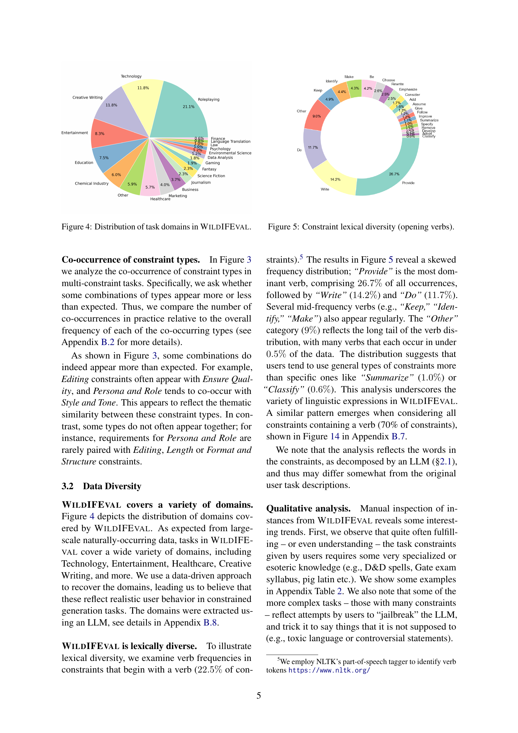
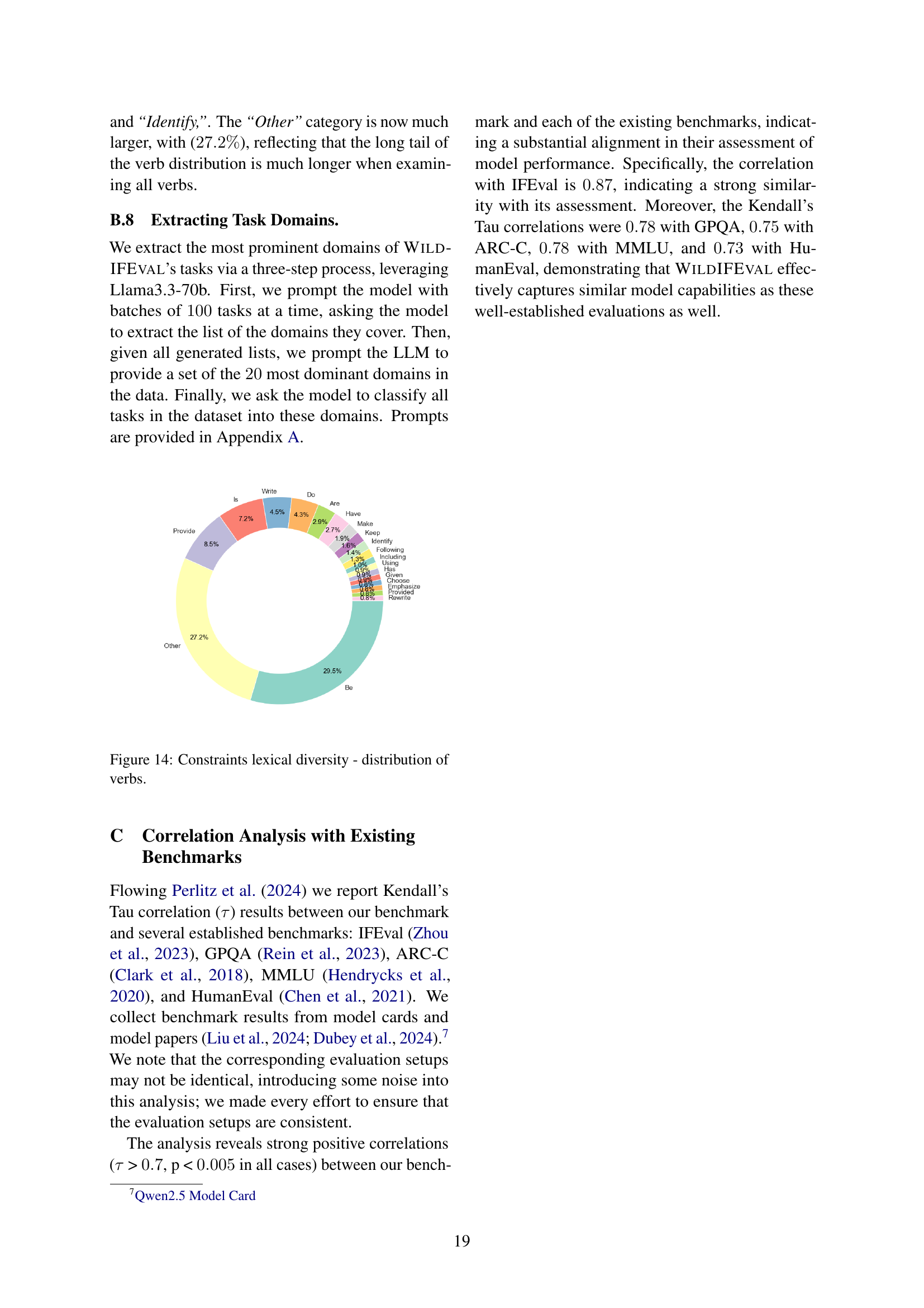
🔼 This figure shows the distribution of different domains present in the WildIFEVAL dataset. It provides a visual representation of the variety of real-world tasks included in the dataset, categorized by their subject matter. This allows readers to quickly understand the range of topics the dataset covers, which influences the generality of conclusions drawn from the dataset. The visual representation helps in assessing the diversity and real-world applicability of the benchmark.
read the caption
Figure 4: Distribution of task domains in WildIFEval.

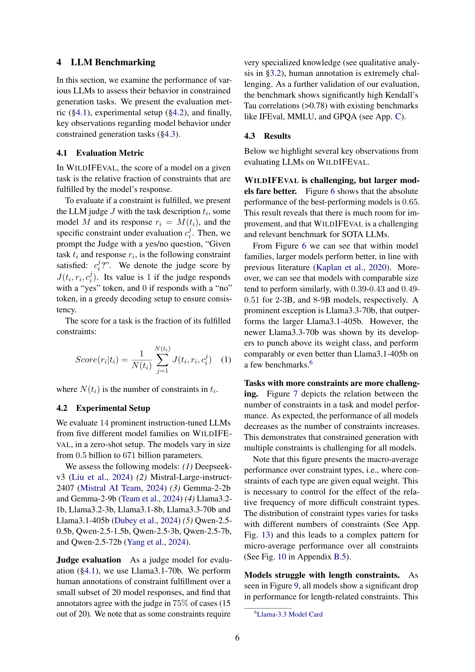
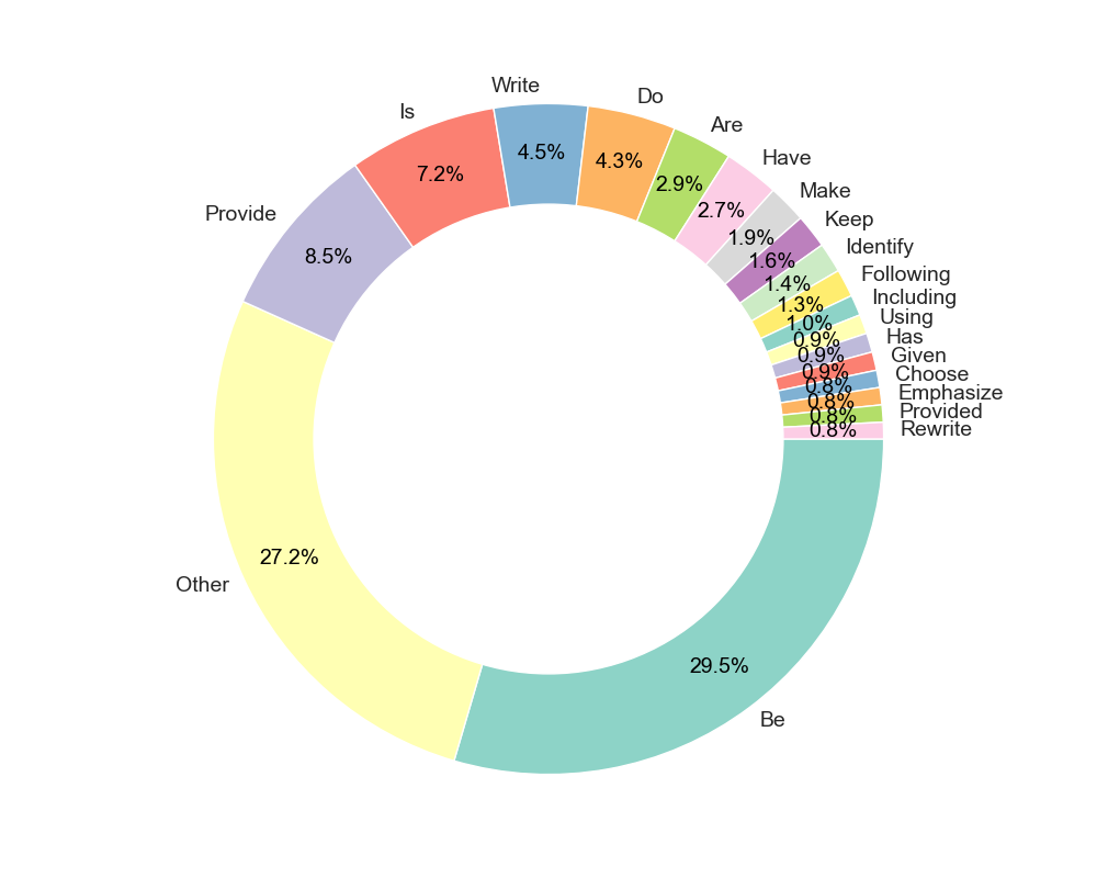
🔼 This figure shows the distribution of the most frequent verbs used at the beginning of constraints within the WILDIFEVAL dataset. It illustrates the lexical diversity of the constraints by showing how often certain verbs are used to initiate user-specified requirements. The visualization allows for a better understanding of the common ways in which users express constraints in natural language.
read the caption
Figure 5: Constraint lexical diversity (opening verbs).

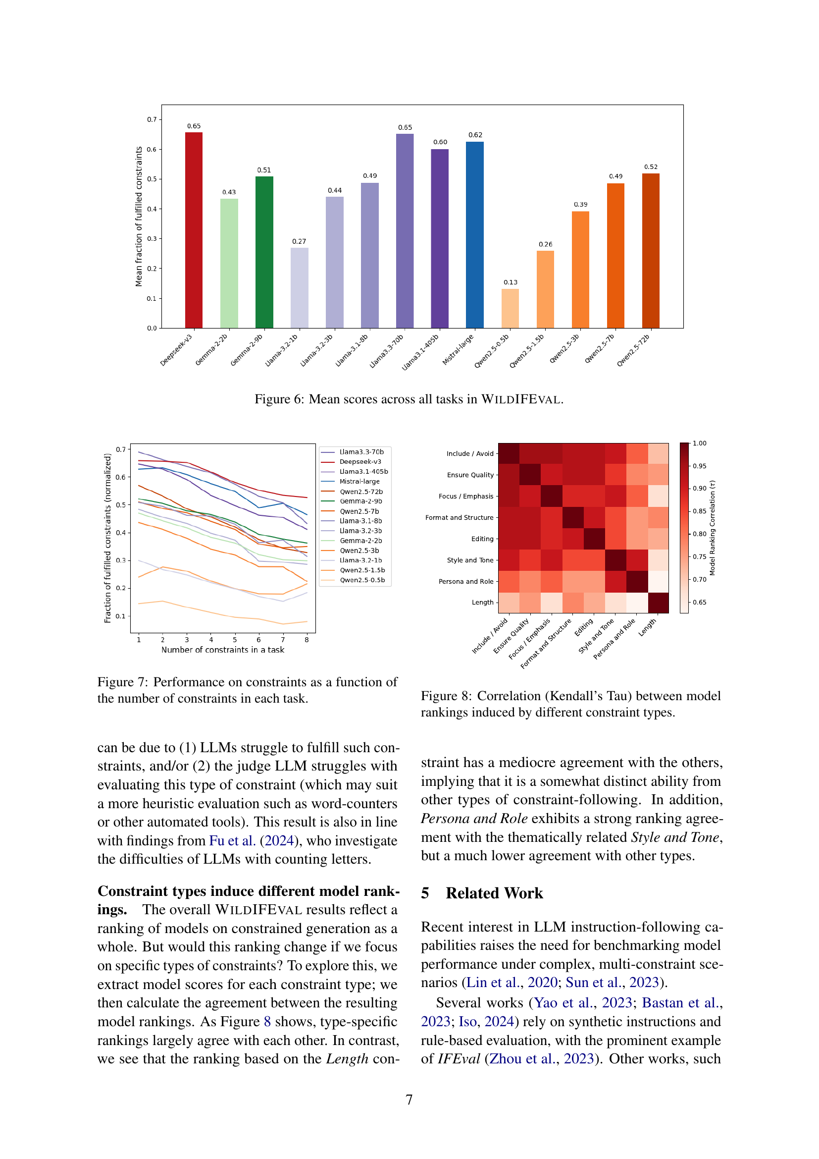
🔼 This figure displays the average performance scores of 14 different Large Language Models (LLMs) across all tasks within the WildIFEval benchmark dataset. Each bar represents an LLM, showing its mean score, indicating the overall effectiveness of the model in fulfilling multiple, real-world constraints presented in user instructions. It provides a high-level view of the relative performance of these models on the challenging multi-constraint instruction-following tasks.
read the caption
Figure 6: Mean scores across all tasks in WildIFEval.

🔼 This figure displays the relationship between the number of constraints in a given task and the model’s performance in fulfilling those constraints. The x-axis represents the number of constraints, while the y-axis shows the fraction of constraints successfully met by the models. Multiple lines are present, each representing a different large language model (LLM), allowing for a comparison of their performance across varying constraint complexities. The graph reveals how the model’s success rate generally declines as the number of constraints increases, indicating that more complex tasks pose greater challenges to LLMs.
read the caption
Figure 7: Performance on constraints as a function of the number of constraints in each task.

🔼 This figure displays the correlation between model rankings generated using different constraint types from the WILDIFEVAL dataset. Kendall’s Tau, a measure of rank correlation, is used to quantify the agreement between these rankings. A higher correlation indicates a greater similarity in how different models perform across various constraint types. This helps to understand whether models struggle consistently across all constraint types, or if their performance varies significantly depending on the specific type of constraint.
read the caption
Figure 8: Correlation (Kendall’s Tau) between model rankings induced by different constraint types.

🔼 This figure displays the average performance of several large language models (LLMs) across eight different constraint categories in a constrained text generation task. The y-axis represents the fraction of fulfilled constraints (a measure of how well the LLMs satisfied the specified requirements), and the x-axis lists the eight constraint types. The figure highlights the relative strengths and weaknesses of different LLMs when handling various types of constraints. Note that this figure presents a subset of the models analyzed; the complete results, including smaller models, are found in Figure 12 of the Appendix.
read the caption
Figure 9: Mean constraint-following performance by constraint category. Here we focus on a subset of large models, the full version is in Figure 12 in the Appendix.

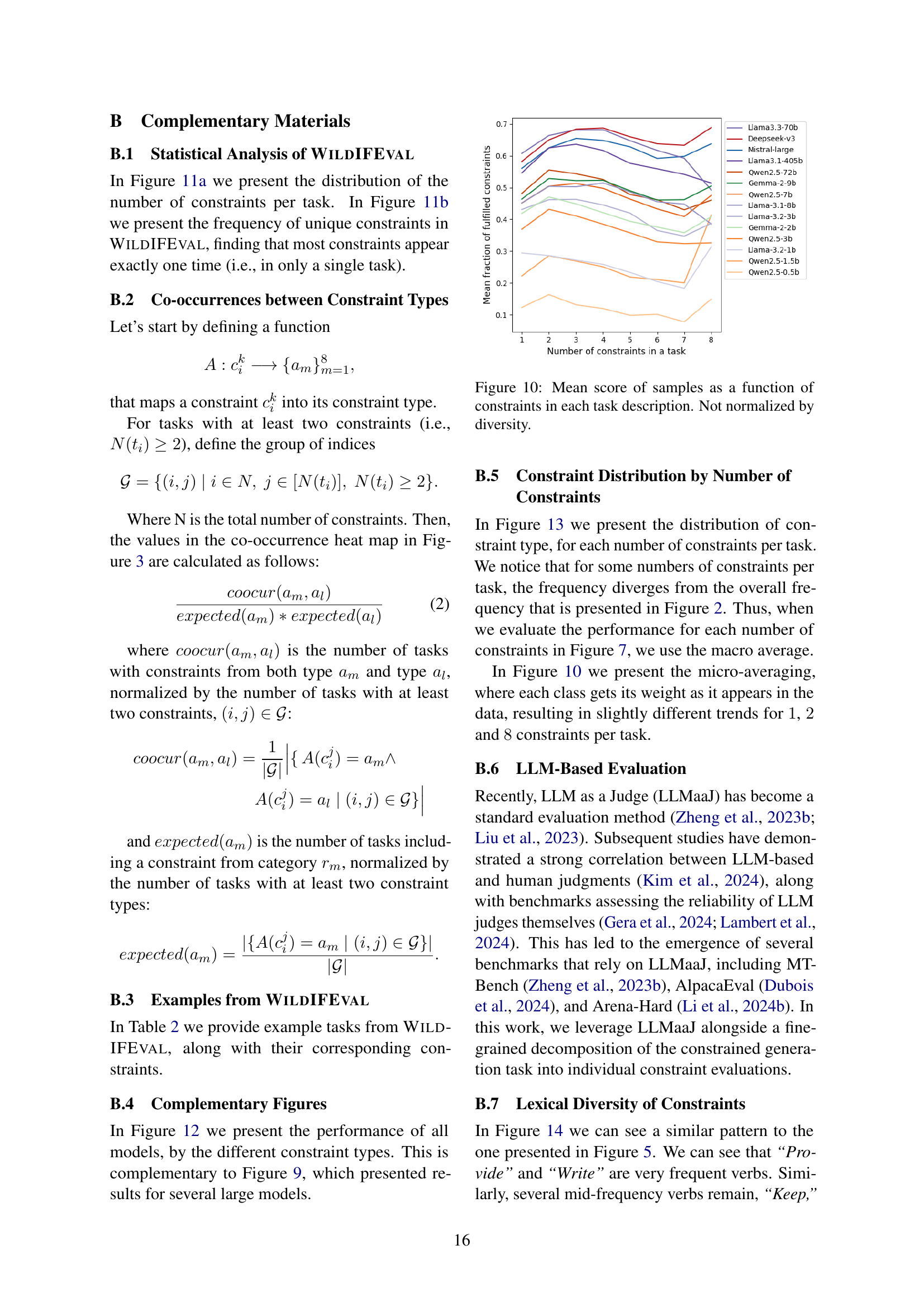
🔼 This figure displays the average performance of different language models on tasks with varying numbers of constraints. The x-axis represents the number of constraints in a task, and the y-axis shows the mean score achieved by the models on those tasks. The scores are not adjusted for the diversity of constraint types within each task. This visualization helps to understand how the difficulty of a task increases with the number of constraints imposed.
read the caption
Figure 10: Mean score of samples as a function of constraints in each task description. Not normalized by diversity.

🔼 The figure shows the distribution of constraint types in the WILDIFEVAL dataset. The bar chart visually represents the frequency of each constraint type, offering a clear understanding of their prevalence in real-world user instructions. This provides insight into the common types of constraints users employ when interacting with LLMs, highlighting the most frequent and least frequent types.
read the caption
(a)
🔼 This figure is a t-SNE projection of the embeddings of constraints from the WILDIFEVAL dataset, colored by their type. It visually represents the relationships between different types of constraints. Constraints of similar types cluster together, while those of different types are more spread out. This visualization helps to understand the semantic similarity and diversity within the different constraint categories in the dataset.
read the caption
(b)

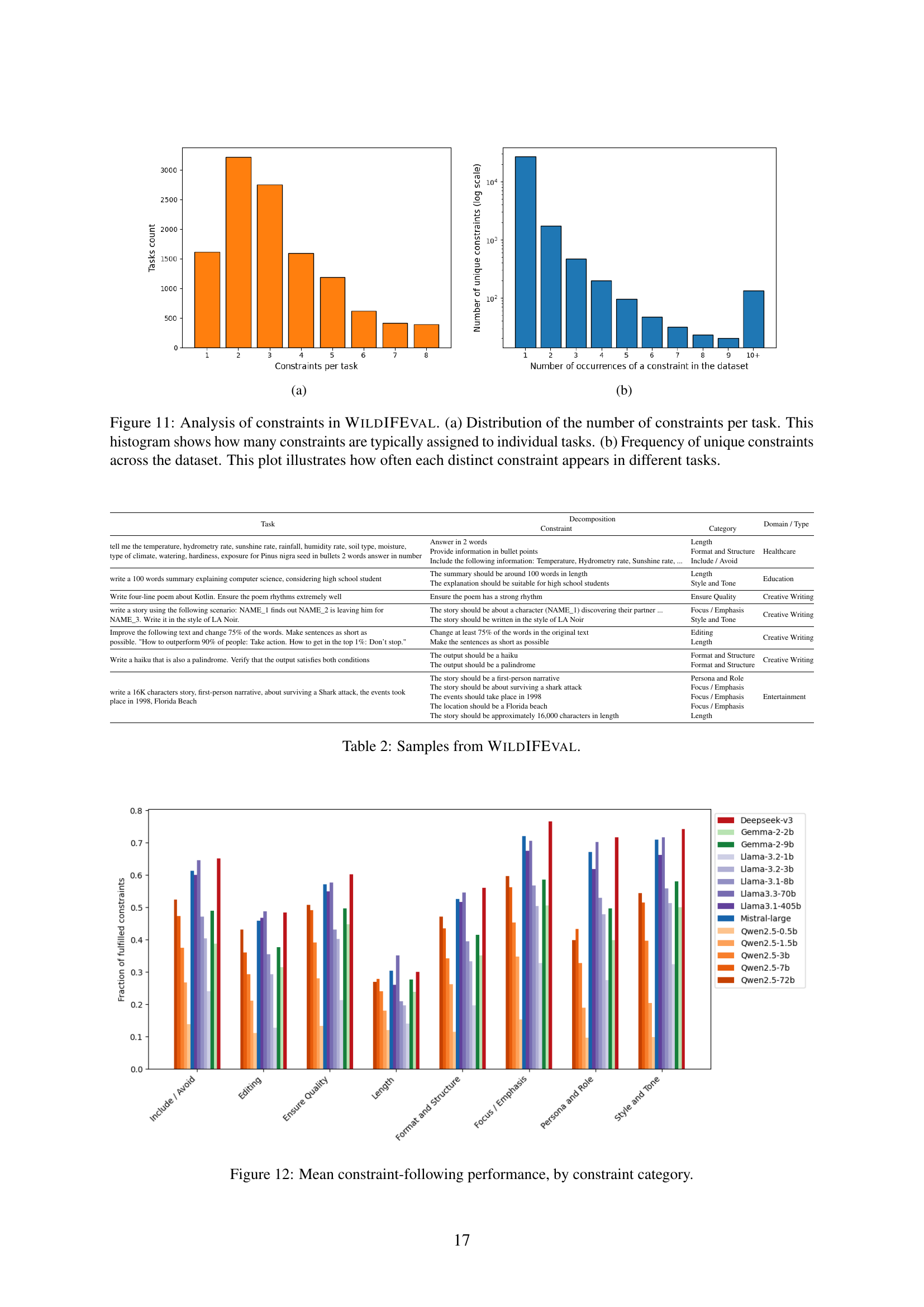
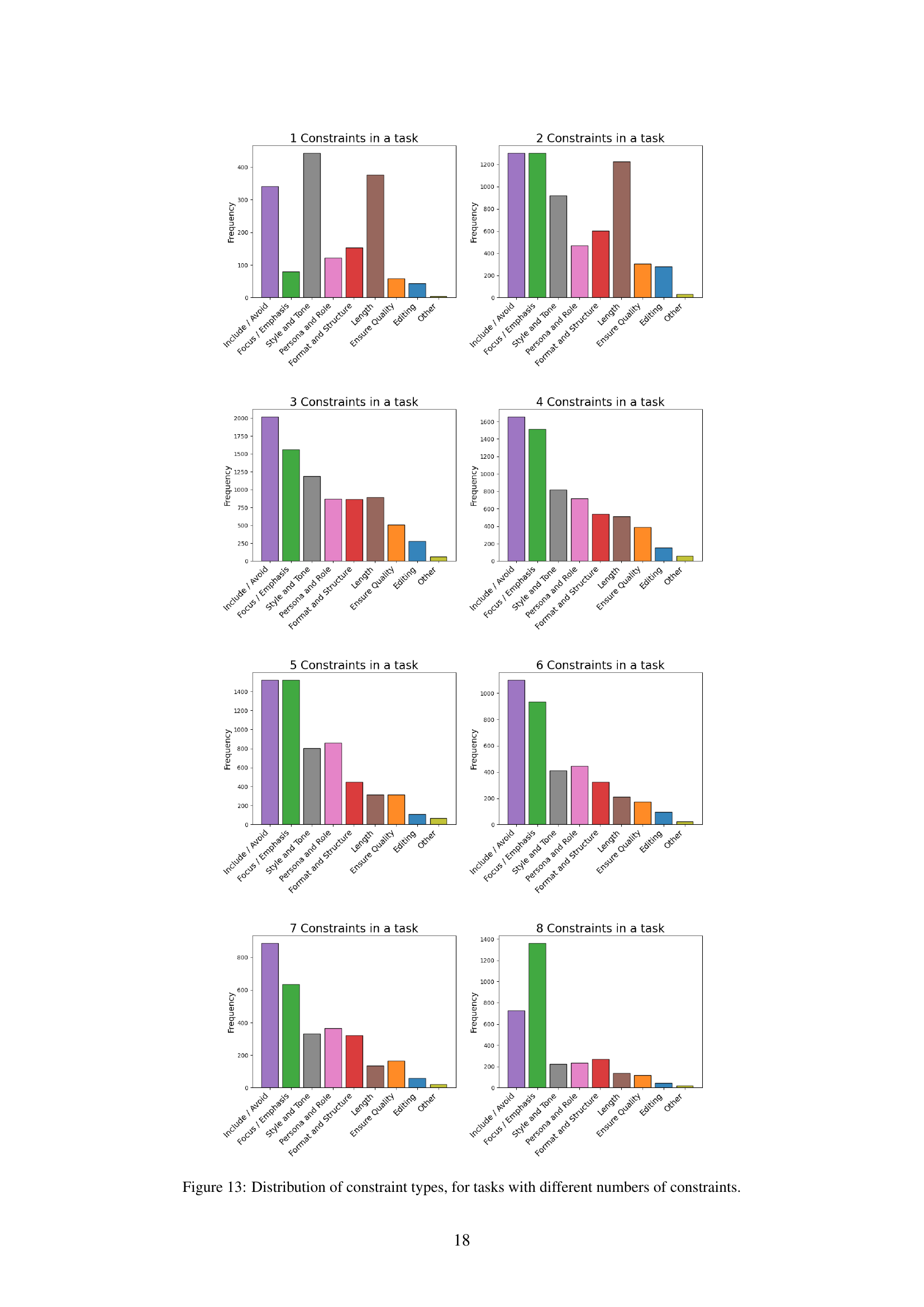
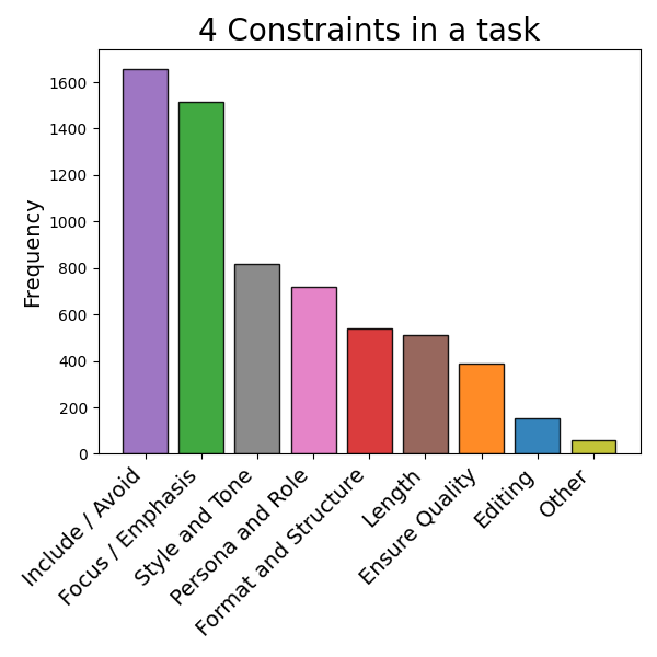
🔼 Figure 11 presents a dual analysis of constraints within the WildIFEval dataset. The first sub-figure (a) displays a histogram showing the distribution of the number of constraints per task, illustrating the typical number of constraints found in each task within the dataset. The second sub-figure (b) presents a bar chart illustrating the frequency distribution of unique constraints across all tasks. This visualizes how often each individual constraint appears in the dataset, highlighting the prevalence of various types of constraints and indicating whether certain types are more common than others.
read the caption
Figure 11: Analysis of constraints in WildIFEval. (a) Distribution of the number of constraints per task. This histogram shows how many constraints are typically assigned to individual tasks. (b) Frequency of unique constraints across the dataset. This plot illustrates how often each distinct constraint appears in different tasks.

🔼 This figure displays the average performance of various LLMs across different constraint categories in the WILDIFEVAL benchmark. Each bar represents a constraint type (e.g., length, style, focus), and the bar height shows the mean proportion of successfully fulfilled constraints of that type by the different LLMs. The x-axis lists the different constraint types, and the y-axis shows the average performance. It helps to illustrate which constraint types are more challenging for LLMs to satisfy.
read the caption
Figure 12: Mean constraint-following performance, by constraint category.

🔼 Distribution of constraint types in the WILDIFEVAL dataset. The bar chart shows the frequency of each of eight constraint types found in the dataset. This visualization helps to understand the relative prevalence of different types of constraints within real-world user instructions for text generation tasks.
read the caption
(a)

🔼 This figure shows a t-SNE projection of the embeddings of constraints from the WILDIFEVAL dataset, colored by their type. It visually represents the semantic similarity between different constraint types. Constraints of similar types (e.g., Format and Structure, Length, Style and Tone) cluster together, indicating semantic closeness. In contrast, constraints related to content (e.g., Include/Avoid, Focus/Emphasis) are more spread out, highlighting their diversity and less structured nature.
read the caption
(b)
🔼 This figure displays the Kendall’s Tau correlation coefficients between the model rankings produced by WILDIFEVAL and several other established benchmarks. Higher values indicate stronger agreement between the rankings. The benchmarks compared are IFEval, GPQA, ARC-C, MMLU, and HumanEval, showing a high degree of correlation with WILDIFEVAL, suggesting that the benchmark effectively measures similar model capabilities.
read the caption
(c)
Full paper#