TL;DR#
Masked image generation models offer promise, but existing approaches have limitations. MaskGIT suffers from information loss due to discrete tokenization, while MAR falls short of VAR in limited sampling steps. Masked diffusion models (MDMs) show potential in text generation, but their applicability to image generation is unclear. Existing methods are either inefficient, lack scalability, or are not applicable to various data types.
This paper introduces eMIGM, a unified framework integrating masked image modeling and masked diffusion models. eMIGM systematically explores training and sampling strategies, optimizing performance and efficiency. Key innovations include higher masking ratios, a weighting function inspired by MaskGIT/MAE, CFG with Mask, and a time interval strategy for classifier-free guidance. eMIGM demonstrates strong performance on ImageNet generation, outperforming VAR and achieving comparable results to continuous diffusion models with less compute.
Key Takeaways#
Why does it matter?#
This paper is important for researchers because it unifies masked image generation and masked diffusion models, providing a more efficient and scalable approach. The reduced computational cost and strong performance on high-resolution images open new possibilities for generative modeling research.
Visual Insights#

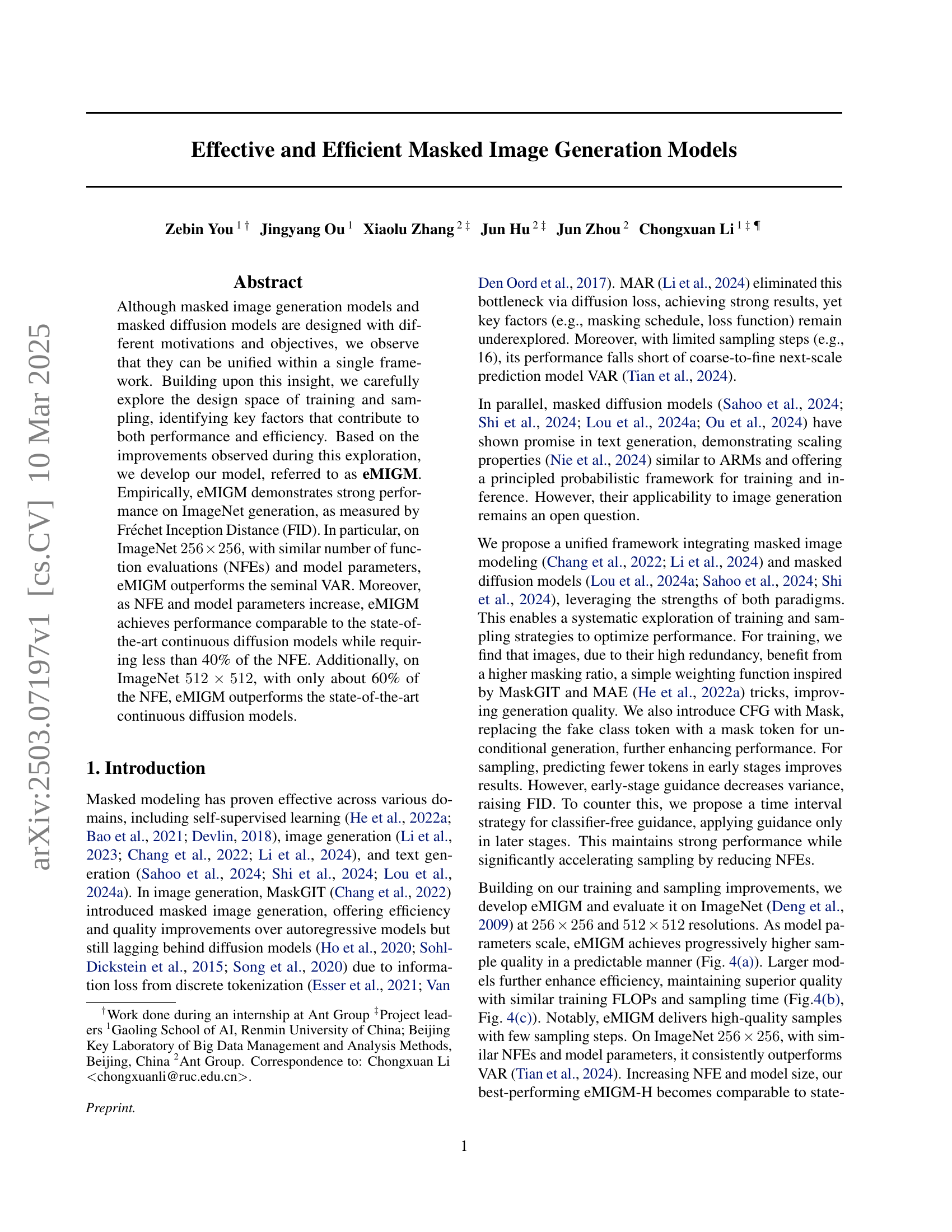
🔼 This figure displays various images generated by the eMIGM model. The model was trained using the ImageNet dataset, specifically at a resolution of 512x512 pixels. The images showcase the model’s ability to generate diverse and realistic images, representing a range of objects and scenes from the ImageNet dataset. The quality and variety of the generated samples are used to demonstrate the effectiveness of the eMIGM model.
read the caption
Figure 1: Generated samples from eMIGM trained on ImageNet 512×512512512512\times 512512 × 512.
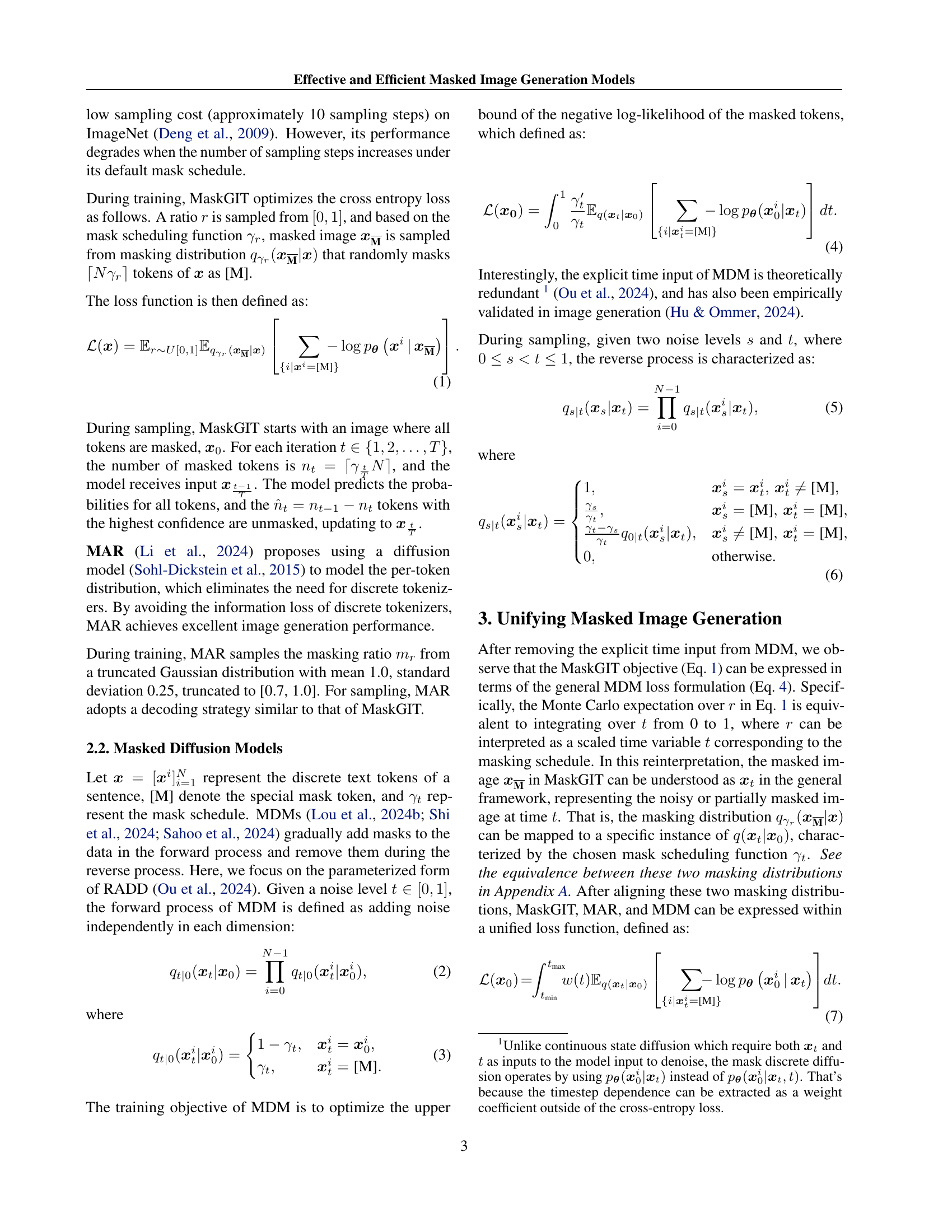
| Method | Masking Distribution | Weighting Function | Conditional Distribution |
|---|---|---|---|
| MaskGIT | Uniformly mask tokens w/o replacement | Categorical Distribution | |
| MAR | Uniformly mask tokens w/o replacement | Diffusion Model | |
| MDM | Mask tokens independently with ratio | Categorical Distribution |
🔼 This table compares three different masked image generation models (MaskGIT, MAR, and MDM) within a unified framework. The key differences between the models are highlighted by showing how they differ in their choices of three components: 1) the masking distribution, which determines how the input image is masked during training; 2) the weighting function, which assigns weights to the loss at different time steps during training; and 3) the conditional distribution, which represents the model’s prediction of the original unmasked image given the masked input. By examining these differences, the table clarifies how the individual design choices of each model contribute to its overall performance.
read the caption
Table 1: Comparison of different masked image modeling approaches through a unified framework. The differences among these approaches are defined by the choice of masking distribution q(𝒙t|𝒙0)𝑞conditionalsubscript𝒙𝑡subscript𝒙0q(\boldsymbol{x}_{t}|\boldsymbol{x}_{0})italic_q ( bold_italic_x start_POSTSUBSCRIPT italic_t end_POSTSUBSCRIPT | bold_italic_x start_POSTSUBSCRIPT 0 end_POSTSUBSCRIPT ), weighting function w(t)𝑤𝑡w(t)italic_w ( italic_t ), and conditional distribution p𝜽(𝒙0i∣𝒙t)subscript𝑝𝜽conditionalsuperscriptsubscript𝒙0𝑖subscript𝒙𝑡p_{\boldsymbol{\theta}}(\boldsymbol{x}_{0}^{i}\mid\boldsymbol{x}_{t})italic_p start_POSTSUBSCRIPT bold_italic_θ end_POSTSUBSCRIPT ( bold_italic_x start_POSTSUBSCRIPT 0 end_POSTSUBSCRIPT start_POSTSUPERSCRIPT italic_i end_POSTSUPERSCRIPT ∣ bold_italic_x start_POSTSUBSCRIPT italic_t end_POSTSUBSCRIPT ).
In-depth insights#
Masking Unifying#
The idea of unifying masking is interesting because it provides a common lens through which to view different techniques. It suggests that seemingly disparate methods, like those used in MaskGIT and masked diffusion models (MDMs), may share underlying mechanisms. This unification allows for a more systematic exploration of the design space, potentially leading to insights about which factors contribute most to performance and efficiency. By bridging the gap between discrete and continuous approaches, the study can investigate how different masking strategies impact the learning process and the quality of generated images. A unified framework enables us to consider the advantages of each approach, and to apply the best ideas from each to the problem of image generation. If successful, unifying masking could lead to more efficient and effective methods, and further advancements in masked image generation.
Efficient Masking#
Efficient masking strategies are vital in masked image generation, balancing performance and computational cost. A well-designed masking approach should prioritize information retention while minimizing redundancy. Static masking can be computationally efficient but may not adapt to the varying complexities within an image. Dynamic masking, on the other hand, adjusts the masking ratio based on image content, potentially leading to better results but at a higher cost. The choice of masking ratio is also crucial. Higher ratios encourage the model to learn robust representations from limited context, while lower ratios provide more information, aiding in fine-grained details. It’s essential to explore and optimize masking strategies, including the schedules and masking ratio, to achieve the best trade-off between image quality and computational efficiency. Efficient masking is a critical factor that can lead to accelerated training and sampling without sacrificing generation quality.
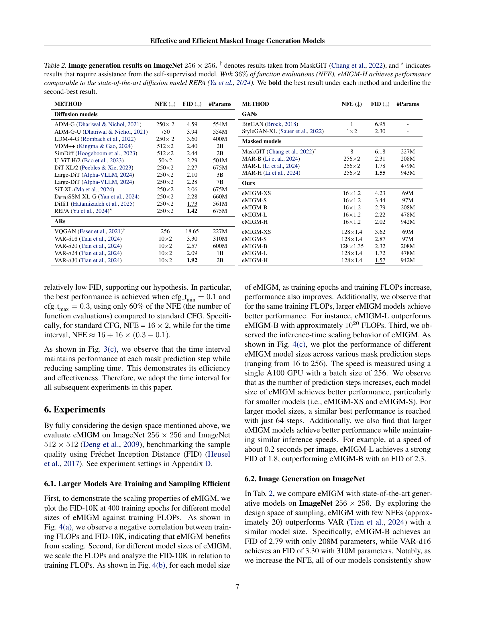
eMIGM Scalability#
eMIGM’s scalability is evident through its performance across ImageNet resolutions. As models scale, a negative correlation between training FLOPs and FID-10K suggests improved sample quality with increased training. Larger models achieve superior quality with the same training FLOPs, indicating training efficiency. Inference speed remains consistent across different model sizes, implying that larger models are more sampling-efficient. These quantitative results underscore eMIGM’s ability to maintain performance and sampling efficiency across diverse resolutions.
CFG Time Interval#
The research uses a time interval strategy for classifier-free guidance (CFG). In MDM, generating tokens is irreversible; early strong guidance can reduce result variations, increasing FID. The method applies CFG only during specific time intervals to maintain performance while reducing sampling time. Experiments validate this approach, showing better results with a controlled CFG application window. By using a time interval, it allows for high variation early on and accurate convergence later, thus resulting in a better FID score and improved generative results. The strategy balances exploration and exploitation in the generation process, enhancing the quality and efficiency of the generated images.
ImageNet Beats#
While the exact heading “ImageNet Beats” isn’t present, the paper extensively discusses the performance of its proposed model, eMIGM, on the ImageNet dataset. A core theme revolves around achieving state-of-the-art or comparable results to existing models, particularly diffusion models and GANs, while demonstrating improved efficiency. The paper highlights eMIGM’s ability to outperform models like VAR with similar computational resources (NFEs) and model parameters. Furthermore, it showcases the model’s scalability, where larger eMIGM models achieve better performance with similar training FLOPs and sampling times. The key contribution lies in efficiently generating high-quality images on ImageNet, surpassing or matching existing methods in terms of FID score with fewer sampling steps or computational resources. This focus on efficiency without sacrificing quality is a major differentiator and a recurring point emphasized throughout the paper’s experimental results and analysis. The comparison with the state-of-the-art showcases the superiority of eMIGM.
More visual insights#
More on figures

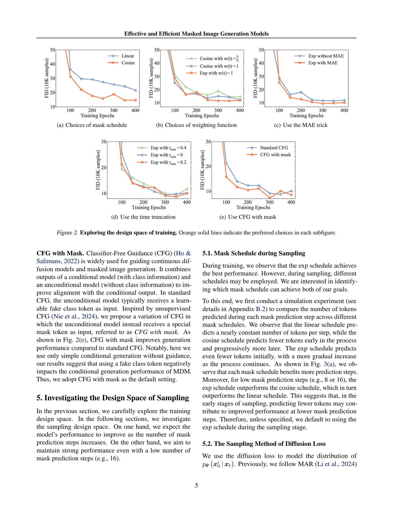
🔼 The figure shows the impact of different mask schedules on the training process of the model. The x-axis represents the training epochs, and the y-axis represents the FID (Fréchet Inception Distance) score, a metric used to evaluate the quality of generated images. Lower FID scores indicate better image quality. Three different mask schedules are compared: Linear, Cosine, and Exp. The results show that the cosine schedule leads to lower FID scores than the linear schedule, and the exp schedule is unstable, indicating that the cosine schedule is the most effective for training.
read the caption
(a) Choices of mask schedule

🔼 This figure compares the performance of different weighting functions used in the loss function during the training process of the masked image generation model. The x-axis represents the training epochs, and the y-axis represents the FID (Fréchet Inception Distance) score, a metric used to evaluate the quality of generated images. The lower the FID score, the better the generated image quality. The figure shows that using a weighting function of w(t) = 1 yields better image quality than w(t) = Yt/sqrt(t), which is used in the original MDM model. This suggests that a simpler weighting function may be more effective for training the masked image generation model.
read the caption
(b) Choices of weighting function
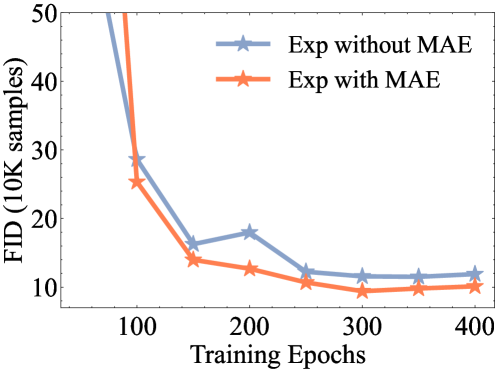
🔼 This figure shows the impact of using the Masked Autoencoder (MAE) architecture on model training. The MAE architecture processes only unmasked tokens, which can improve performance compared to a single-encoder transformer architecture. The x-axis represents training epochs, and the y-axis represents the FID (Fréchet Inception Distance) score. Lower FID values indicate better image generation quality. The figure compares the performance of the model trained with and without the MAE architecture using the exponential masking schedule.
read the caption
(c) Use the MAE trick

🔼 This figure explores the impact of time truncation on the training process of the masked image generation model. Time truncation modifies the minimum value of the time variable ’t’ during training, effectively controlling the minimum masking ratio. The results show the effect of different time truncation values (tmin = 0, 0.2, and 0.4) on the FID (Fréchet Inception Distance) score over training epochs using the exponential masking schedule and the MAE (Masked Autoencoder) architecture, with and without classifier free guidance (CFG) with mask. The optimal value of tmin balances accelerating training convergence with avoiding performance degradation due to excessive masking.
read the caption
(d) Use the time truncation

🔼 This figure shows the effect of using Classifier-Free Guidance (CFG) with a mask token instead of a fake class token on the training performance of the masked image generation model. The graph plots FID (Fréchet Inception Distance) score versus training epochs. The orange line represents the model trained with CFG using a mask token, while the blue line represents the model trained with standard CFG. The results demonstrate that using a mask token with CFG leads to improved performance compared to the standard CFG approach, suggesting that replacing the fake class token with a mask token is beneficial for this type of image generation model.
read the caption
(e) Use CFG with mask

🔼 Figure 2 systematically investigates the impact of various design choices during the training phase of a masked image generation model. Each subfigure focuses on a specific hyperparameter or architectural decision, such as the mask schedule, weighting function, use of the MAE trick, time truncation, and incorporating CFG with a mask. The x-axis typically represents training epochs, and the y-axis usually shows the FID score as a measure of generated image quality. Orange lines highlight the design choices that yield the best performance according to the paper’s experiments. This figure allows the reader to visualize how different choices affect the training process and ultimately, the quality of the generated images.
read the caption
Figure 2: Exploring the design space of training. Orange solid lines indicate the preferred choices in each subfigure.

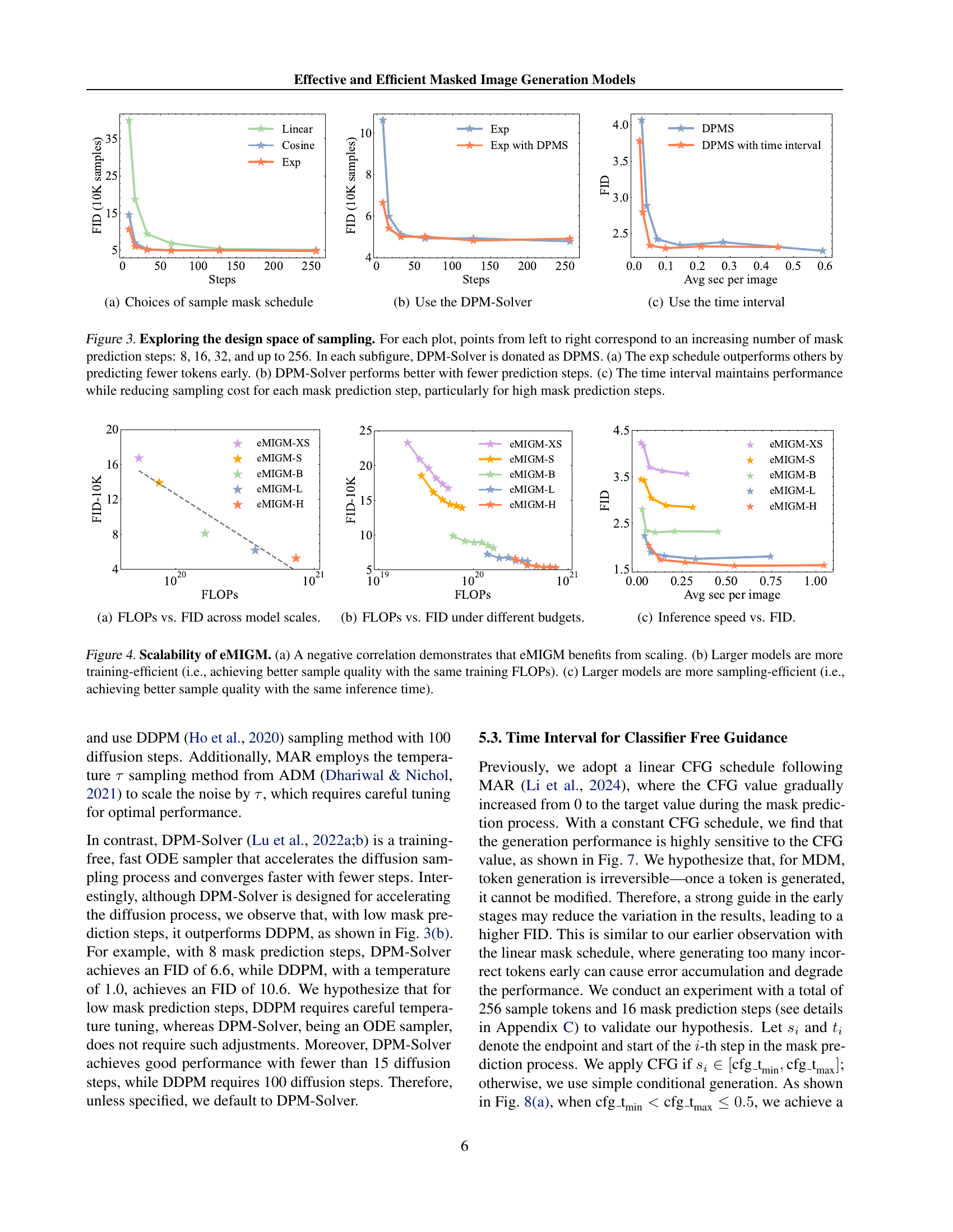
🔼 This figure compares the performance of three different sample mask schedules: linear, cosine, and exponential. The x-axis represents the number of sampling steps, and the y-axis shows the FID score (Fréchet Inception Distance), a metric for evaluating the quality of generated images. Lower FID scores indicate better image quality. The plot shows how the choice of mask schedule affects the generated image quality as the number of sampling steps increases. The results show the relative performance of each mask schedule in the context of the paper’s overall image generation model.
read the caption
(a) Choices of sample mask schedule

🔼 This figure compares the performance of different sampling methods for masked image generation models. Specifically, it shows how the Fréchet Inception Distance (FID) changes as the number of sampling steps increases, when using the DPM-Solver algorithm. The DPM-Solver is an efficient ODE sampler that accelerates the diffusion sampling process and converges faster with fewer steps than other methods like DDPM. The results indicate that DPM-Solver generally outperforms other methods, particularly when fewer sampling steps are used. It demonstrates that DPM-Solver is a suitable method for efficient and high-quality masked image generation.
read the caption
(b) Use the DPM-Solver

🔼 This figure shows the impact of using a time interval strategy for classifier-free guidance (CFG) during sampling. The FID (Fréchet Inception Distance) is plotted against the number of training epochs for different CFG approaches: the standard CFG, and CFG with time intervals (tmin=0, tmin=0.2, and tmin=0.4). The time interval strategy applies CFG only to later stages of sampling, which improves efficiency by reducing function evaluations (NFEs) while maintaining performance. The results demonstrate that a time interval of tmin=0.2 provides the best balance of efficiency and performance.
read the caption
(c) Use the time interval

🔼 This figure explores the impact of different sampling strategies on the performance of masked image generation models. It shows how the choice of mask schedule (linear, cosine, exponential), the sampling method (DPM-Solver vs. standard diffusion), and the use of a time interval for classifier-free guidance affect FID scores across varying numbers of mask prediction steps (8, 16, 32, …, 256). The exponential mask schedule is highlighted for predicting fewer tokens in earlier steps, improving efficiency. DPM-Solver is demonstrated to be superior, especially with fewer sampling steps. Finally, the time-interval approach for classifier-free guidance shows that it can maintain FID performance while significantly reducing sampling costs.
read the caption
Figure 3: Exploring the design space of sampling. For each plot, points from left to right correspond to an increasing number of mask prediction steps: 8, 16, 32, and up to 256. In each subfigure, DPM-Solver is donated as DPMS. (a) The exp schedule outperforms others by predicting fewer tokens early. (b) DPM-Solver performs better with fewer prediction steps. (c) The time interval maintains performance while reducing sampling cost for each mask prediction step, particularly for high mask prediction steps.

🔼 This figure shows the relationship between FLOPs (floating point operations) and FID (Fréchet Inception Distance) for different scales of the eMIGM model. The x-axis represents the number of FLOPs during training, while the y-axis shows the FID score, a measure of generated image quality (lower is better). The plot reveals how the model’s performance (FID) improves as the model size increases (more FLOPs are used during training). This demonstrates the scaling properties of the eMIGM model, showing that larger models achieve better image generation quality with increased computational cost.
read the caption
(a) FLOPs vs. FID across model scales.

🔼 This figure shows the relationship between FLOPs (floating-point operations) and FID (Fréchet Inception Distance) for different model sizes of eMIGM, under various computational budget constraints. Each point represents a model with different FLOPs and the corresponding FID. It illustrates the trade-off between model size and generation quality. The trend shows that generally higher FLOPs lead to lower FID (better image quality), however the figure also highlights the relative efficiency of larger models, showing how well they perform given a certain FLOP budget.
read the caption
(b) FLOPs vs. FID under different budgets.

🔼 This figure shows the relationship between the inference speed (time taken to generate one image) and the Fréchet Inception Distance (FID), a measure of image quality. Faster inference speeds are desirable, but ideally without sacrificing image quality (a lower FID score is better). The plot likely shows how inference time changes as the size of the eMIGM model increases, suggesting that larger models may be more efficient at generating high-quality images. Different points on the graph likely represent different model sizes.
read the caption
(c) Inference speed vs. FID.

🔼 Figure 4 demonstrates the scalability and efficiency of the eMIGM model. Panel (a) shows a negative correlation between the model size (measured in FLOPs) and the Fréchet Inception Distance (FID) score, indicating that larger models generally produce higher-quality images (lower FID). Panel (b) highlights the training efficiency of eMIGM; larger models achieve better image quality with the same number of training FLOPs, demonstrating improved training efficiency as model size increases. Finally, panel (c) showcases the sampling efficiency: larger models maintain high image quality while using less inference time, indicating that larger models are more efficient during the inference phase (image generation).
read the caption
Figure 4: Scalability of eMIGM. (a) A negative correlation demonstrates that eMIGM benefits from scaling. (b) Larger models are more training-efficient (i.e., achieving better sample quality with the same training FLOPs). (c) Larger models are more sampling-efficient (i.e., achieving better sample quality with the same inference time).

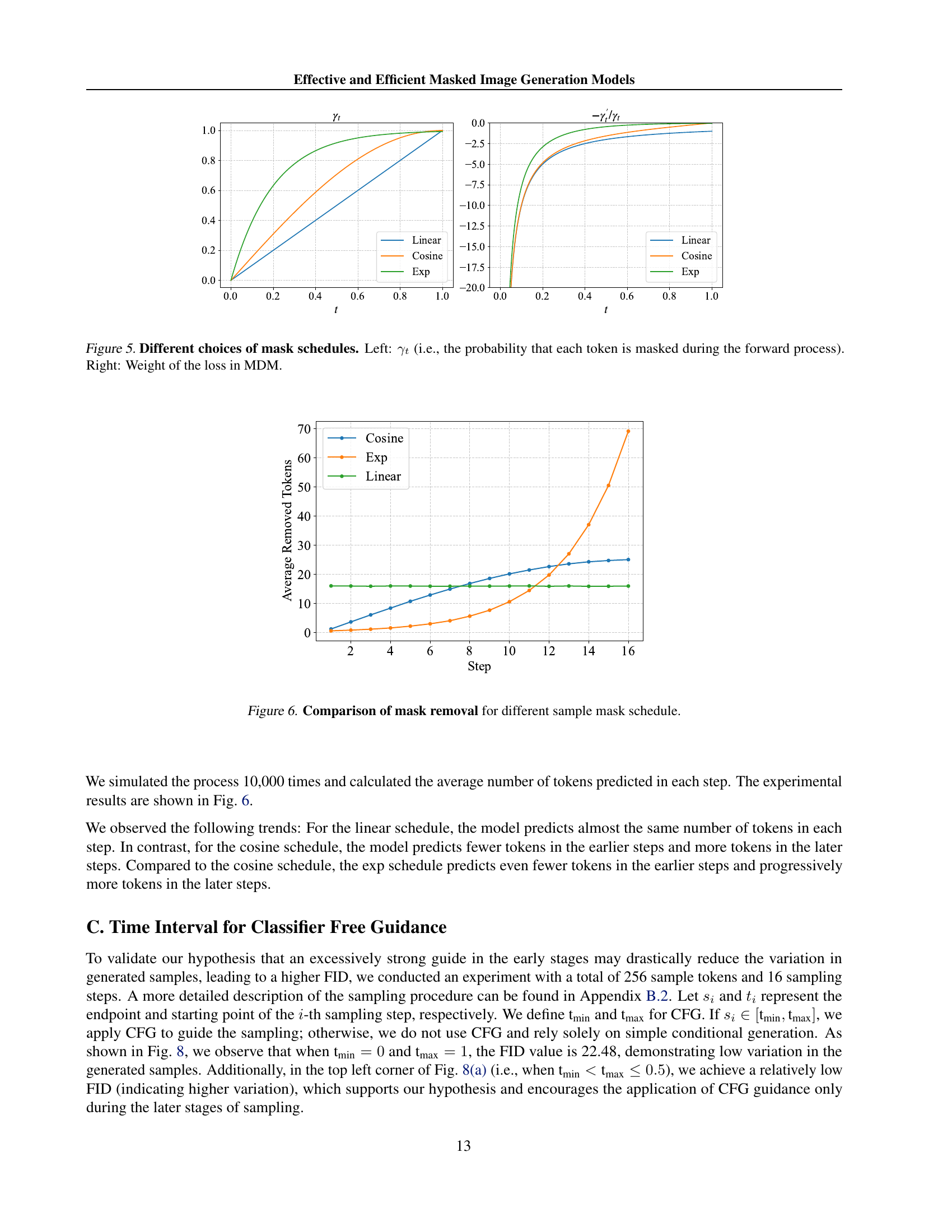
🔼 This figure compares three different mask schedules: linear, cosine, and exponential. The left panel shows the probability of masking a token (γt) at different time steps (t) for each schedule. The right panel shows the weight (w(t)) assigned to the loss function at each time step, which is also determined by the mask schedule. The different functions are to illustrate the relationship between the probability of masking a token and the weight associated with the loss in the masked diffusion model (MDM). The choice of mask schedule affects both the training process and the quality of the generated images.
read the caption
Figure 5: Different choices of mask schedules. Left: γtsubscript𝛾𝑡\gamma_{t}italic_γ start_POSTSUBSCRIPT italic_t end_POSTSUBSCRIPT (i.e., the probability that each token is masked during the forward process). Right: Weight of the loss in MDM.

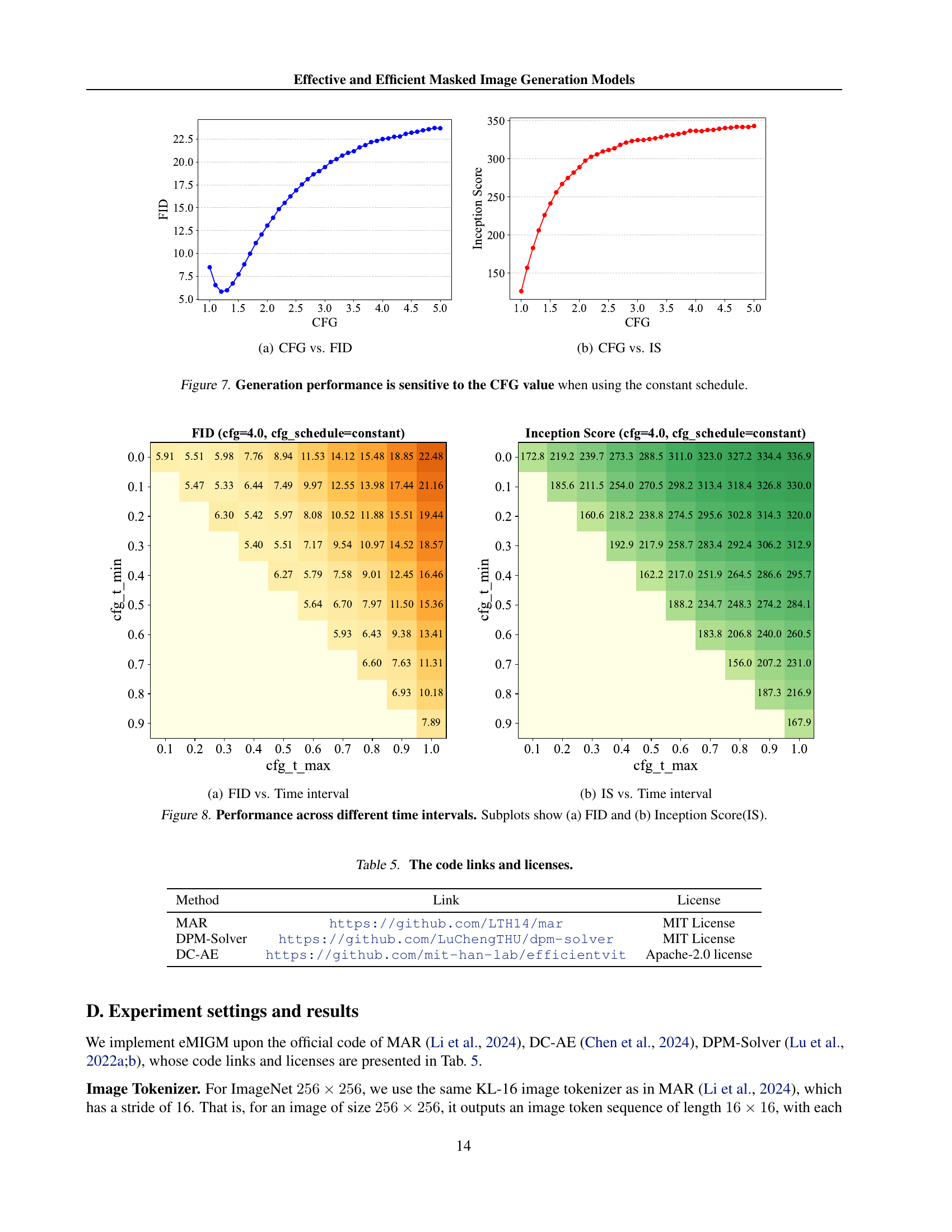
🔼 This figure shows the average number of tokens predicted at each step during the sampling process for three different mask schedules: linear, cosine, and exponential. The x-axis represents the sampling step, and the y-axis represents the average number of tokens removed. The linear schedule shows a relatively constant number of tokens removed at each step. The cosine schedule removes fewer tokens in the early steps and progressively more in later steps. The exponential schedule removes the fewest tokens in the early steps and gradually increases the number of tokens removed as sampling progresses.
read the caption
Figure 6: Comparison of mask removal for different sample mask schedule.

🔼 This figure shows the relationship between classifier-free guidance (CFG) and Fréchet Inception Distance (FID) scores. The x-axis represents different CFG values, and the y-axis represents the FID score. Lower FID scores indicate better image quality. The plot helps to determine the optimal CFG value that balances image quality and generation speed. This analysis is important because strong guidance can sometimes decrease the diversity and realism of generated images, while insufficient guidance can hurt the quality.
read the caption
(a) CFG vs. FID
More on tables
| METHOD | NFE () | FID () | #Params |
|---|---|---|---|
| Diffusion models | |||
| ADM-G [13] | 250 2 | 4.59 | 554M |
| ADM-G-U [13] | 750 | 3.94 | 554M |
| LDM-4-G [40] | 250 2 | 3.60 | 400M |
| VDM++ [27] | 5122 | 2.40 | 2B |
| SimDiff [24] | 5122 | 2.44 | 2B |
| U-ViT-H/2 [3] | 502 | 2.29 | 501M |
| DiT-XL/2 [39] | 2502 | 2.27 | 675M |
| Large-DiT [1] | 2502 | 2.10 | 3B |
| Large-DiT [1] | 2502 | 2.28 | 7B |
| SiT-XL [36] | 2502 | 2.06 | 675M |
| DSSM-XL-G [50] | 2502 | 2.28 | 660M |
| DiffiT [17] | 2502 | 1.73 | 561M |
| REPA [51]⋆ | 2502 | 1.42 | 675M |
| ARs | |||
| VQGAN [14]† | 256 | 18.65 | 227M |
| VAR- [48] | 102 | 3.30 | 310M |
| VAR- [48] | 102 | 2.57 | 600M |
| VAR- [48] | 102 | 2.09 | 1B |
| VAR- [48] | 102 | 1.92 | 2B |
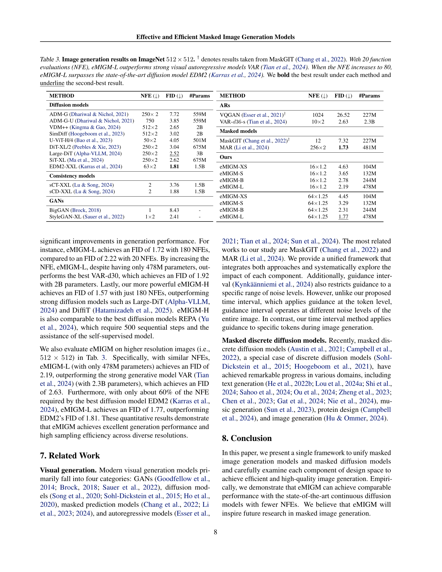
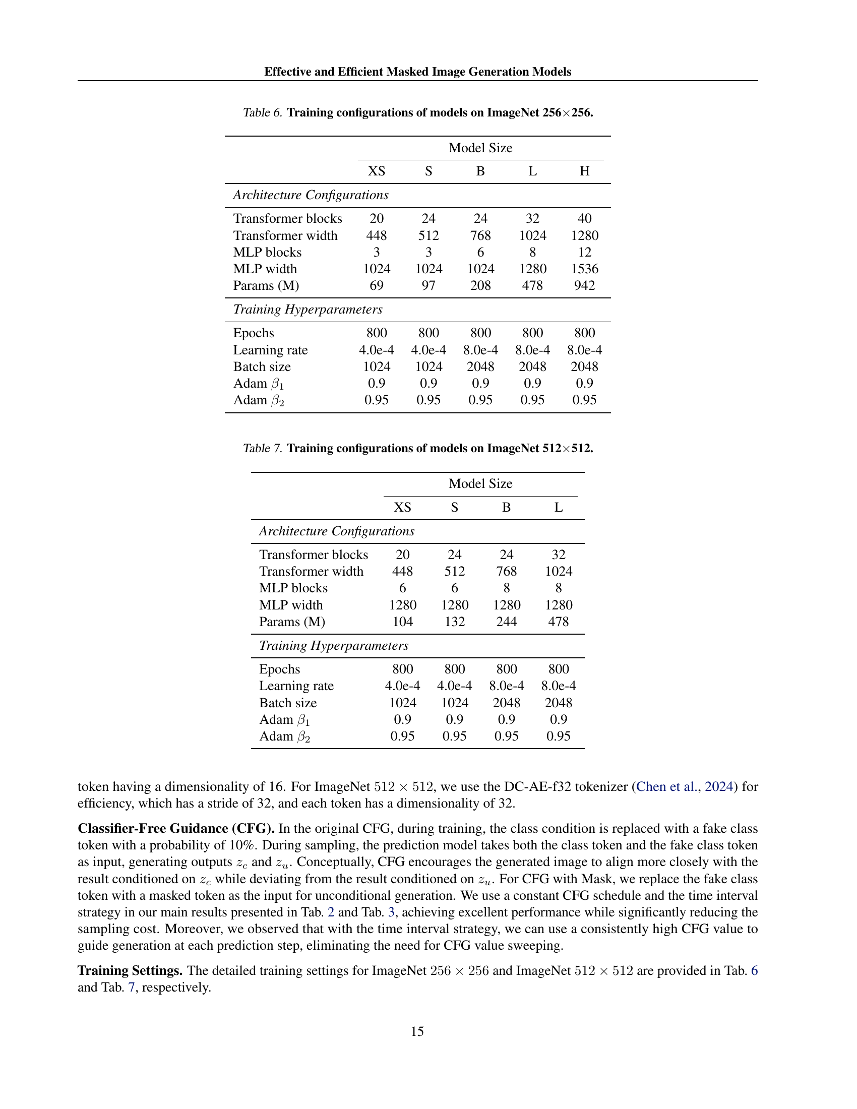
🔼 Table 2 presents a comparison of various image generation models’ performance on the ImageNet 256x256 dataset. The models are categorized into diffusion models, GANs, masked models, and the proposed eMIGM model and its variants. Key metrics include FID (Fréchet Inception Distance) score, the number of function evaluations (NFEs), and model parameters. Lower FID scores indicate better image quality, fewer NFEs signify greater efficiency, and parameters represent model size. Results from MaskGIT and models requiring self-supervised assistance are noted. The table highlights eMIGM-H’s competitive performance, achieving state-of-the-art results with only 36% of the function evaluations used by the best-performing competitor.
read the caption
Table 2: Image generation results on ImageNet 256×256256256256\times 256256 × 256. † denotes results taken from MaskGIT [8], and ⋆ indicates results that require assistance from the self-supervised model. With 36%percent3636\%36 % of function evaluations (NFE), eMIGM-H achieves performance comparable to the state-of-the-art diffusion model REPA [51]. We bold the best result under each method and underline the second-best result.
| METHOD | NFE () | FID () | #Params |
|---|---|---|---|
| GANs | |||
| BigGAN [5] | 1 | 6.95 | - |
| StyleGAN-XL [42] | 12 | 2.30 | - |
| Masked models | |||
| MaskGIT [8]† | 8 | 6.18 | 227M |
| MAR-B [30] | 256 | 2.31 | 208M |
| MAR-L [30] | 256 | 1.78 | 479M |
| MAR-H [30] | 256 | 1.55 | 943M |
| Ours | |||
| eMIGM-XS | 161.2 | 4.23 | 69M |
| eMIGM-S | 161.2 | 3.44 | 97M |
| eMIGM-B | 161.2 | 2.79 | 208M |
| eMIGM-L | 161.2 | 2.22 | 478M |
| eMIGM-H | 161.2 | 2.02 | 942M |
| eMIGM-XS | 1281.4 | 3.62 | 69M |
| eMIGM-S | 1281.4 | 2.87 | 97M |
| eMIGM-B | 1281.35 | 2.32 | 208M |
| eMIGM-L | 1281.4 | 1.72 | 478M |
| eMIGM-H | 1281.4 | 1.57 | 942M |
🔼 This table presents a comparison of various image generation models’ performance on the ImageNet 512x512 dataset. The key metrics are FID (Fréchet Inception Distance), a measure of generated image quality, and NFE (Number of Function Evaluations), representing computational cost. The table compares several diffusion models, masked models (including MaskGIT, which is referenced), and generative adversarial networks (GANs). It shows how the FID score improves as the number of function evaluations increases for the proposed eMIGM model, demonstrating its ability to generate high-quality images with increasing computational resources. The best FID scores for each model category are highlighted.
read the caption
Table 3: Image generation results on ImageNet 512×512512512512\times 512512 × 512. † denotes results taken from MaskGIT [8]. With 20 function evaluations (NFE), eMIGM-L outperforms strong visual autoregressive models VAR [48]. When the NFE increases to 80, eMIGM-L surpasses the state-of-the-art diffusion model EDM2 [26]. We bold the best result under each method and underline the second-best result.
| METHOD | NFE () | FID () | #Params |
|---|---|---|---|
| Diffusion models | |||
| ADM-G [13] | 250 2 | 7.72 | 559M |
| ADM-G-U [13] | 750 | 3.85 | 559M |
| VDM++ [27] | 5122 | 2.65 | 2B |
| SimDiff [24] | 5122 | 3.02 | 2B |
| U-ViT-H/4 [3] | 502 | 4.05 | 501M |
| DiT-XL/2 [39] | 2502 | 3.04 | 675M |
| Large-DiT [1] | 2502 | 2.52 | 3B |
| SiT-XL [36] | 2502 | 2.62 | 675M |
| EDM2-XXL [26] | 632 | 1.81 | 1.5B |
| Consistency models | |||
| sCT-XXL [33] | 2 | 3.76 | 1.5B |
| sCD-XXL [33] | 2 | 1.88 | 1.5B |
| GANs | |||
| BigGAN [5] | 1 | 8.43 | - |
| StyleGAN-XL [42] | 12 | 2.41 | - |
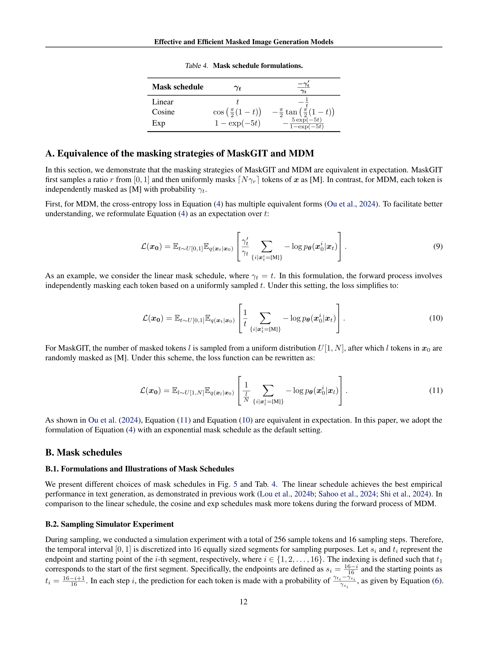
🔼 This table presents the mathematical formulas for three different mask schedules used in the masked image generation model: Linear, Cosine, and Exp. For each schedule, it shows the formula for calculating the probability (γt) that each token will be masked in the forward process, and the weighting function (w(t)) used in the loss function.
read the caption
Table 4: Mask schedule formulations.
| METHOD | NFE () | FID () | #Params |
|---|---|---|---|
| ARs | |||
| VQGAN [14]† | 1024 | 26.52 | 227M |
| VAR--s [48] | 102 | 2.63 | 2.3B |
| Masked models | |||
| MaskGIT [8]† | 12 | 7.32 | 227M |
| MAR [30] | 256 | 1.73 | 481M |
| Ours | |||
| eMIGM-XS | 161.2 | 4.63 | 104M |
| eMIGM-S | 161.2 | 3.65 | 132M |
| eMIGM-B | 161.2 | 2.78 | 244M |
| eMIGM-L | 161.2 | 2.19 | 478M |
| eMIGM-XS | 641.25 | 4.45 | 104M |
| eMIGM-S | 641.25 | 3.29 | 132M |
| eMIGM-B | 641.25 | 2.31 | 244M |
| eMIGM-L | 641.25 | 1.77 | 478M |
🔼 This table provides the links to the source code repositories and the respective licenses for the following projects that are related to or used in the paper: MAR, DPM-Solver, and DC-AE.
read the caption
Table 5: The code links and licenses.
| Mask schedule | ||
|---|---|---|
| Linear | ||
| Cosine | ||
| Exp |
🔼 This table details the specific hyperparameters used during the training process of four different sized models (XS, S, B, L, H) on the ImageNet 256x256 dataset. It includes architecture specifications such as the number of transformer blocks, transformer width, MLP blocks, MLP width, and the total number of parameters in millions. Additionally, it lists the training hyperparameters: epochs, learning rate, batch size, and Adam optimization parameters (β1 and β2).
read the caption
Table 6: Training configurations of models on ImageNet 256×\times×256.
| Method | Link | License |
|---|---|---|
| MAR | https://github.com/LTH14/mar | MIT License |
| DPM-Solver | https://github.com/LuChengTHU/dpm-solver | MIT License |
| DC-AE | https://github.com/mit-han-lab/efficientvit | Apache-2.0 license |
🔼 This table details the different hyperparameters used during the training process of the eMIGM models on ImageNet 512x512. It shows how various architectural choices, including the number of transformer blocks, transformer and MLP widths, and the number of epochs, learning rate, batch size, and Adam optimizer settings (beta1 and beta2), were adjusted across different model sizes (XS, S, B, L). These configurations demonstrate the scalability of the model architecture and training process for large-scale image generation tasks.
read the caption
Table 7: Training configurations of models on ImageNet 512×\times×512.
Full paper#