TL;DR#
LLMs improve reasoning using more test-time computation, but existing fine-tuning methods don’t effectively utilize this computation. Standard outcome-reward RL optimizes for the final result, neglecting intermediate progress, leading to inefficient token use & inability to solve hard problems. This causes unnecessarily long outputs & struggles in making steady progress.
To address these issues, this paper presents Meta Reinforcement Fine-Tuning (MRT). MRT minimizes cumulative regret by optimizing a dense reward function that values progress at each step, alongside the final outcome. This leads to a 2-3x performance gain & 1.5x token efficiency for math reasoning compared to standard RL, offering a new avenue for future explorations.
Key Takeaways#
Why does it matter?#
This paper introduces a novel meta-RL framework (MRT) for optimizing test-time compute in LLMs, achieving superior performance & token efficiency in math reasoning. It offers new research directions of exploring reward structures for more efficient LLMs.
Visual Insights#

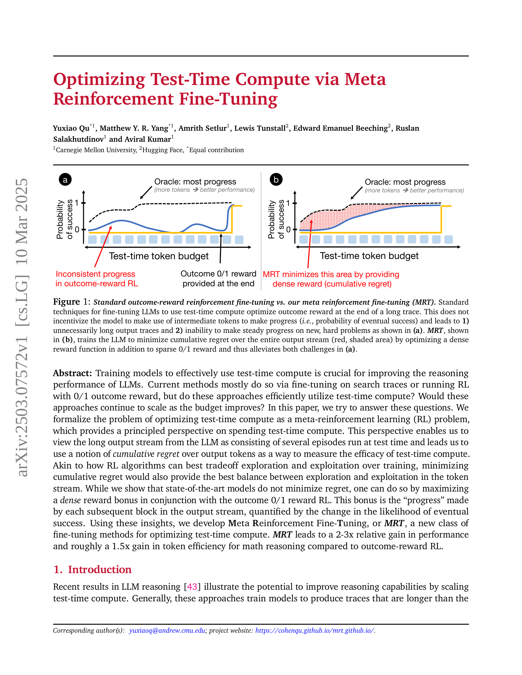
🔼 This figure compares two approaches for fine-tuning large language models (LLMs) to optimize their use of computation during reasoning. The standard approach (a) uses a sparse reward at the end of the process, which leads to unnecessarily long reasoning chains and inconsistent progress. The new method, MRT (b), uses a dense reward function to incentivize progress throughout the reasoning process. The shaded area represents the cumulative regret, which MRT aims to minimize. This allows for more efficient use of computation and more consistent progress, even on difficult problems.
read the caption
Figure 1: Standard outcome-reward reinforcement fine-tuning vs. our meta reinforcement fine-tuning (MRT). Standard techniques for fine-tuning LLMs to use test-time compute optimize outcome reward at the end of a long trace. This does not incentivize the model to make use of intermediate tokens to make progress (i.e., probability of eventual success) and leads to 1) unnecessarily long output traces and 2) inability to make steady progress on new, hard problems as shown in (a). MRT, shown in (b), trains the LLM to minimize cumulative regret over the entire output stream (red, shaded area) by optimizing a dense reward function in addition to sparse 0/1 reward and thus alleviates both challenges in (a).
| Base model + Approach | AIME 2024 | AIME 2025 | AMC 2023 | MinervaMATH | MATH500 | Avg. |
|---|---|---|---|---|---|---|
| DeepScaleR-1.5B-Preview | 42.8 | 36.7 | 83.0 | 24.6 | 85.2 | 54.5 |
| outcome-reward RL (GRPO) | 44.5 (+1.7) | 39.3 (+2.6) | 81.5 (1.5) | 24.7 | 84.9 | 55.0 (+0.5) |
| length penalty | 40.3 (2.5) | 30.3 (6.4) | 77.3 (5.7) | 23.0 | 83.2 | 50.8 (3.7) |
| MRT (Ours) | 47.2 (+4.4) | 39.7 (+3.0) | 83.1 (+0.1) | 24.2 | 85.1 | 55.9 (+1.4) |
| R1-Distill-Qwen-1.5B | 28.7 | 26.0 | 69.9 | 19.8 | 80.1 | 44.9 |
| outcome-reward RL (GRPO) | 29.8 (+1.1) | 27.3 (+1.3) | 70.5 (+0.6) | 22.1 | 80.3 | 46.0 (+1.1) |
| MRT (Ours) | 30.3 (+1.6) | 29.3 (+3.3) | 72.9 (+3.0) | 22.5 | 80.4 | 47.1 (+2.2) |
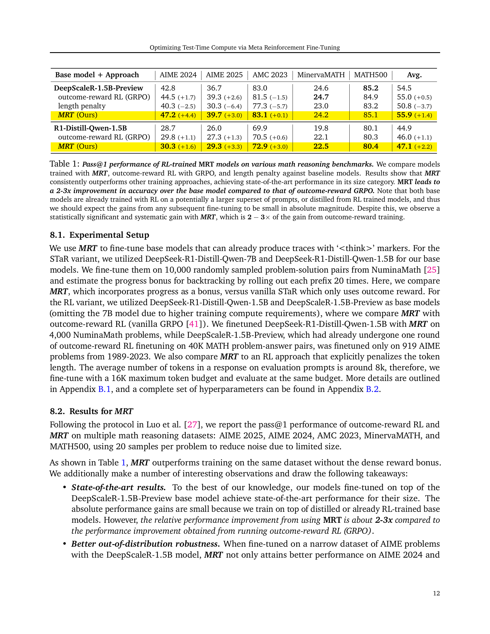
🔼 This table presents the results of the Pass@1 evaluation metric across multiple math reasoning benchmarks. The evaluation compares the performance of models trained using three different methods: Meta Reinforcement Fine-Tuning (MRT), outcome-reward reinforcement learning (RL) with GRPO, and an approach using length penalties. The models are evaluated against baseline models. The results demonstrate that MRT consistently surpasses the other training methods, achieving state-of-the-art accuracy for its model size. Specifically, MRT shows a 2-3 times improvement in accuracy over the baseline models compared to the outcome-reward RL method. It’s important to note that the baseline models were already trained using RL, potentially on a larger dataset; thus, improvements from further fine-tuning are expected to be modest. Despite this, the gains achieved by MRT are statistically significant and consistently exceed the gains from using outcome-reward training.
read the caption
Table 1: Pass@1 performance of RL-trained MRT models on various math reasoning benchmarks. We compare models trained with MRT, outcome-reward RL with GRPO, and length penalty against baseline models. Results show that MRT consistently outperforms other training approaches, achieving state-of-the-art performance in its size category. MRT leads to a 2-3x improvement in accuracy over the base model compared to that of outcome-reward GRPO. Note that both base models are already trained with RL on a potentially a larger superset of prompts, or distilled from RL trained models, and thus we should expect the gains from any subsequent fine-tuning to be small in absolute magnitude. Despite this, we observe a statistically significant and systematic gain with MRT, which is 𝟐−𝟑×\mathbf{2-3\times}bold_2 - bold_3 × of the gain from outcome-reward training.
In-depth insights#
Meta-RL Compute#
Meta-Reinforcement Learning (Meta-RL) for test-time compute focuses on learning how to efficiently use computational resources during inference. Unlike standard RL that optimizes for a final outcome, Meta-RL for compute aims to make steady progress with each step. It is crucial to balance exploration (trying new approaches) and exploitation (refining existing ones) within a token budget. By minimizing the cumulative regret over the output token stream, Meta-RL can strike the best balance between these aspects. Existing methods may not effectively minimize regret or utilize test-time compute well. Meta-RL addresses this by rewarding progress at each step. A dense reward bonus, based on progress, enables the model to learn a budget-agnostic strategy that works well across various computational constraints.
Regret Minimizing#
In the realm of reinforcement learning, ‘regret minimizing’ is a cornerstone concept. It encapsulates the objective of an agent to perform as close as possible to the optimal strategy, thus limiting the cumulative difference (regret) between its actual rewards and those attainable under the ideal policy. This involves balancing exploration of uncharted territories with exploitation of known reward-generating actions. Achieving low regret often relies on strategies like upper confidence bound (UCB) or Thompson sampling, which guide agents to make informed decisions under uncertainty. Furthermore, it underscores the importance of efficient learning, allowing the model to adapt and make smart and optimal decisions based on it’s accumulated experience. Regret minimization can have far-reaching results and can be applied to many complex problems.
Test-Time Scaling#
Test-time scaling involves strategically increasing computational resources during inference to enhance model performance. The paper references earlier work leveraging separate verifier models and beam search, showcasing a shift from simply scaling data or model size to more sophisticated inference techniques. Recent approaches also explore fine-tuning LLMs to “simulate” in-context test-time search. A key challenge highlighted is the limitation of gains due to potential memorization when fine-tuning on search traces, emphasizing the need for methods that promote genuine reasoning rather than rote recall. The authors address this with a warmstart procedure before on-policy STaR/RL to prevent models from memorization.
Backtrack Search#
Backtracking search is presented as a structured approach for episode parameterization, contrasting with the open-ended method. It involves alternating between attempting problem-solving and actively seeking errors in prior attempts, guiding strategic backtracking. Key is the model’s ability to detect errors and backtrack effectively, without relying on
Token Efficiency#
Token efficiency emerges as a critical metric for evaluating LLMs in reasoning tasks, moving beyond mere accuracy. It questions how effectively a model utilizes each generated token to progress toward a solution. Traditional outcome-reward RL, while improving accuracy, often leads to token inefficiency, resulting in unnecessarily long traces. MRT addresses this by incentivizing progress at each step. It surpasses outcome rewards by producing solutions using fewer tokens. High token efficiency enables models to tackle complex problems within given budget constraints. Achieving a balance between exploration and exploitation and token expenditure becomes vital for optimizing performance and scalability of LLMs in resource-constrained environments.
More visual insights#
More on figures

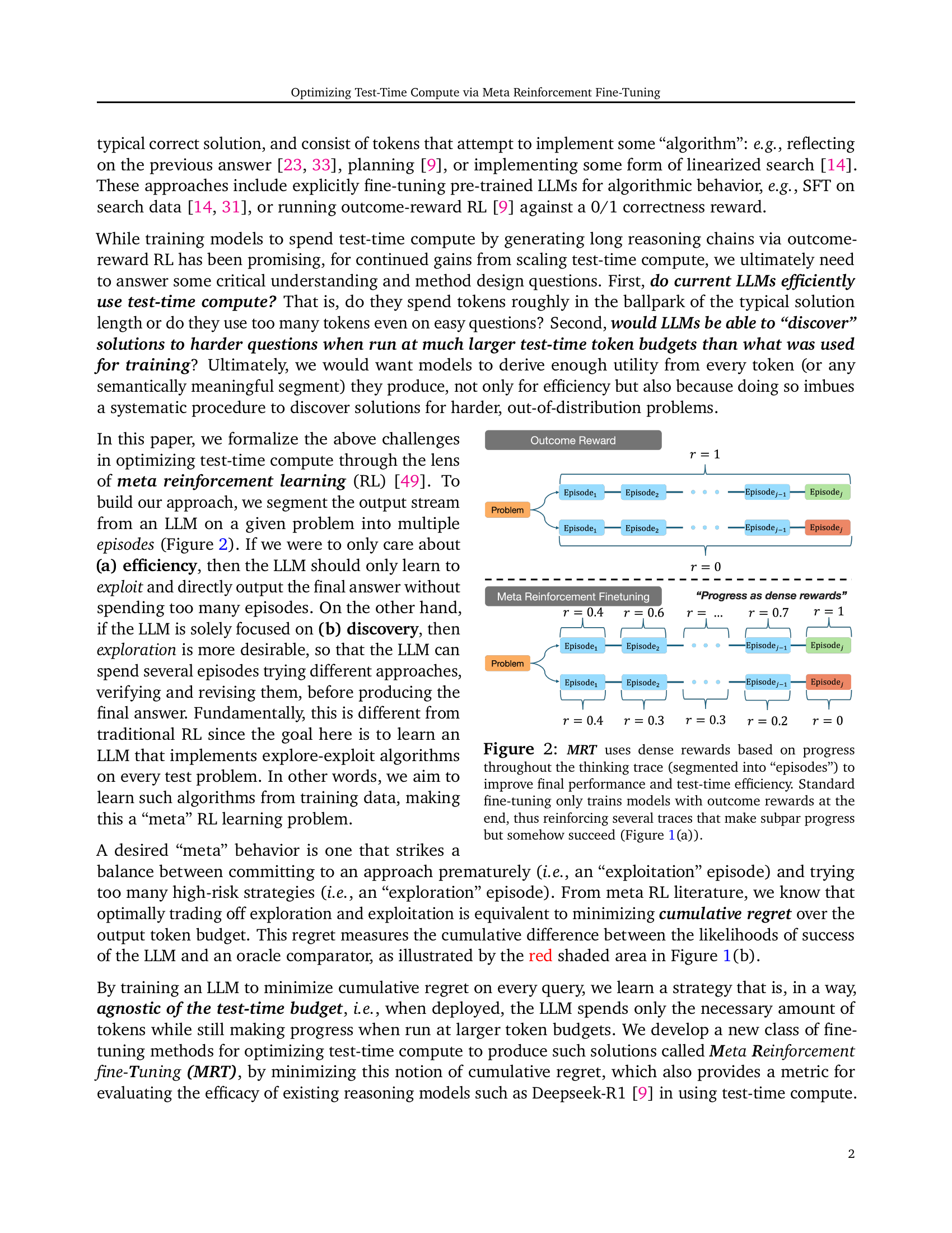
🔼 Figure 2 illustrates the core idea of Meta Reinforcement Fine-Tuning (MRT). Unlike standard fine-tuning which only provides a reward at the end of a reasoning process (a 0/1 outcome reward for success or failure), MRT provides dense (continuous) rewards at each step of the process. This is represented as a progress reward, calculated using the change in the likelihood of success after each step, or episode. The figure demonstrates the difference by contrasting standard outcome reward RL training (a), where long traces might include multiple steps with subpar progress, and MRT (b) which provides dense rewards and minimizes the cumulative regret. This design helps to encourage efficient use of test-time compute, ensuring steady progress toward a solution and avoiding redundant or inefficient steps.
read the caption
Figure 2: MRT uses dense rewards based on progress throughout the thinking trace (segmented into “episodes”) to improve final performance and test-time efficiency. Standard fine-tuning only trains models with outcome rewards at the end, thus reinforcing several traces that make subpar progress but somehow succeed (Figure 1(a)).

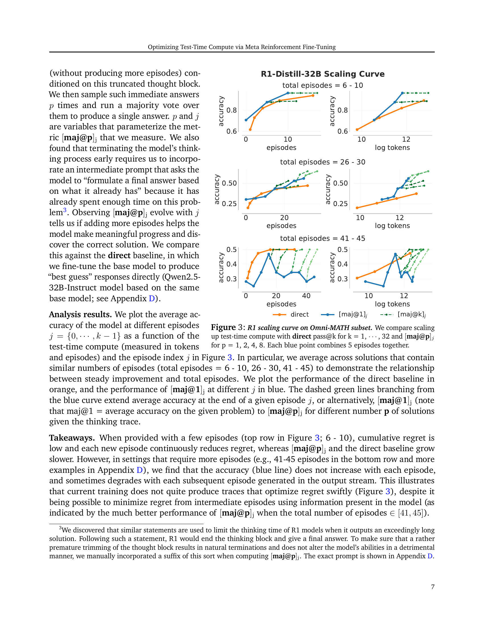
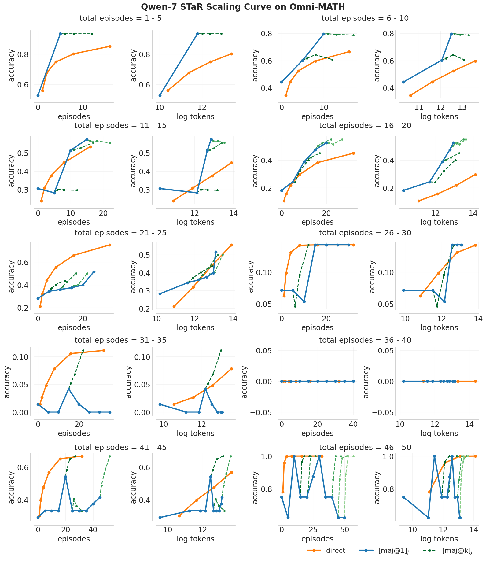
🔼 This figure analyzes how the performance of the DeepSeek-R1 model scales with increasing test-time compute budget on the Omni-MATH dataset. It compares three approaches: 1) directly generating answers (‘direct’), 2) using a single episode with majority voting over multiple runs (’[maj@1]j’), and 3) using multiple episodes with majority voting over multiple runs (’[maj@p]j’). The x-axis represents the test-time token budget, and the y-axis represents the accuracy. The ‘direct’ approach serves as a baseline. The ‘[maj@1]j’ approach evaluates the model’s ability to generate a correct answer within a single episode, and ‘[maj@p]j’ further evaluates its capability to improve the accuracy with multiple episodes. Each blue point on the graph represents an average over 5 episodes.
read the caption
Figure 3: R1 scaling curve on Omni-MATH subset. We compare scaling up test-time compute with direct pass@k for k = 1, ⋯⋯\cdots⋯, 32 and [maj@p]jsubscriptdelimited-[]maj@p𝑗[\textbf{maj@p}]_{j}[ maj@p ] start_POSTSUBSCRIPT italic_j end_POSTSUBSCRIPT for p = 1, 2, 4, 8. Each blue point combines 5 episodes together.

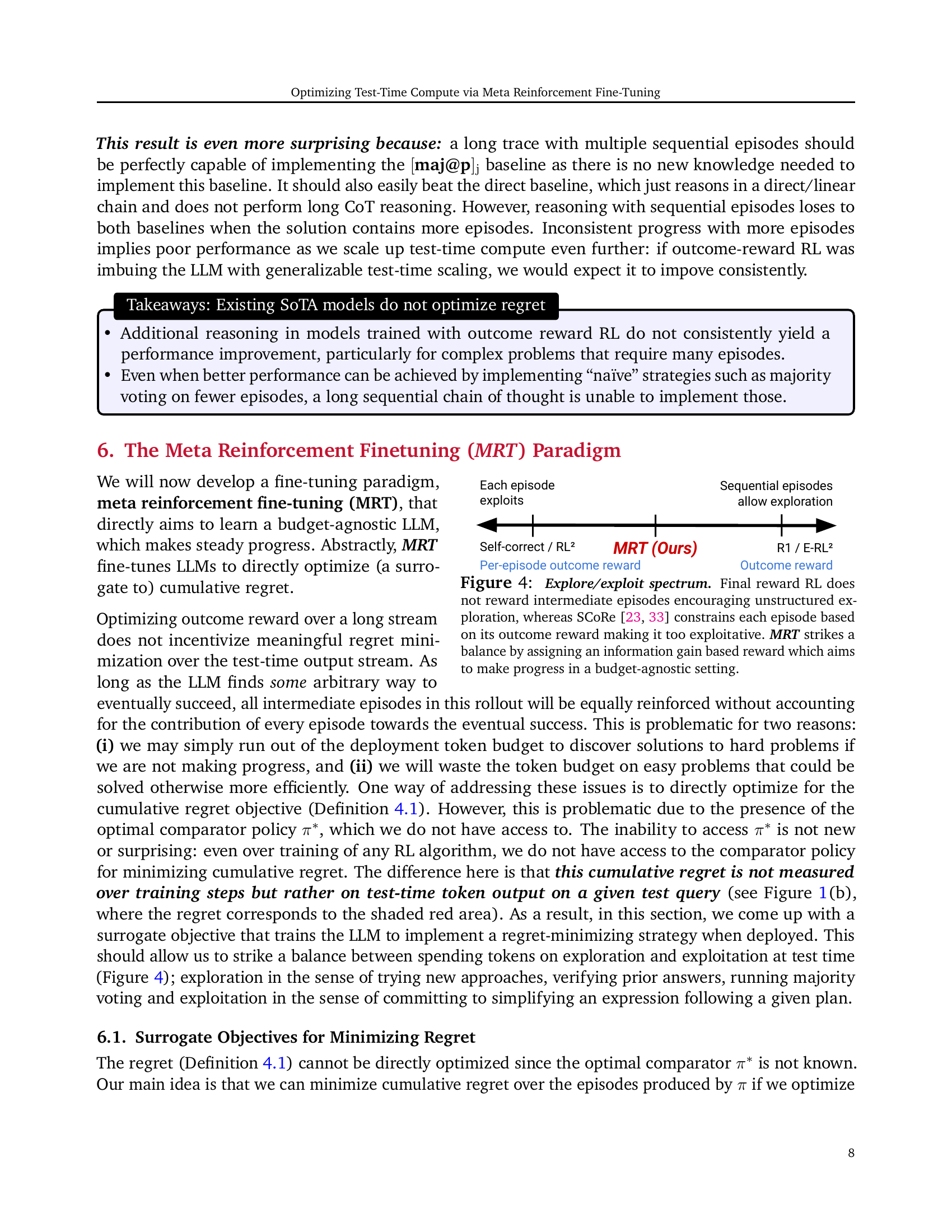
🔼 The figure illustrates the tradeoff between exploration and exploitation in reinforcement learning algorithms for large language models (LLMs). Standard RL methods, focusing solely on the final outcome, incentivize lengthy, unstructured explorations. In contrast, methods like SCoRe prioritize immediate rewards, leading to overly exploitative behavior. MRT, in contrast, seeks a balance. It uses a dense reward bonus that quantifies progress made towards the eventual solution, regardless of the test-time compute budget. This approach encourages exploration of promising paths while discouraging the wasteful expenditure of tokens on unproductive directions.
read the caption
Figure 4: Explore/exploit spectrum. Final reward RL does not reward intermediate episodes encouraging unstructured exploration, whereas SCoRe [23, 33] constrains each episode based on its outcome reward making it too exploitative. MRT strikes a balance by assigning an information gain based reward which aims to make progress in a budget-agnostic setting.

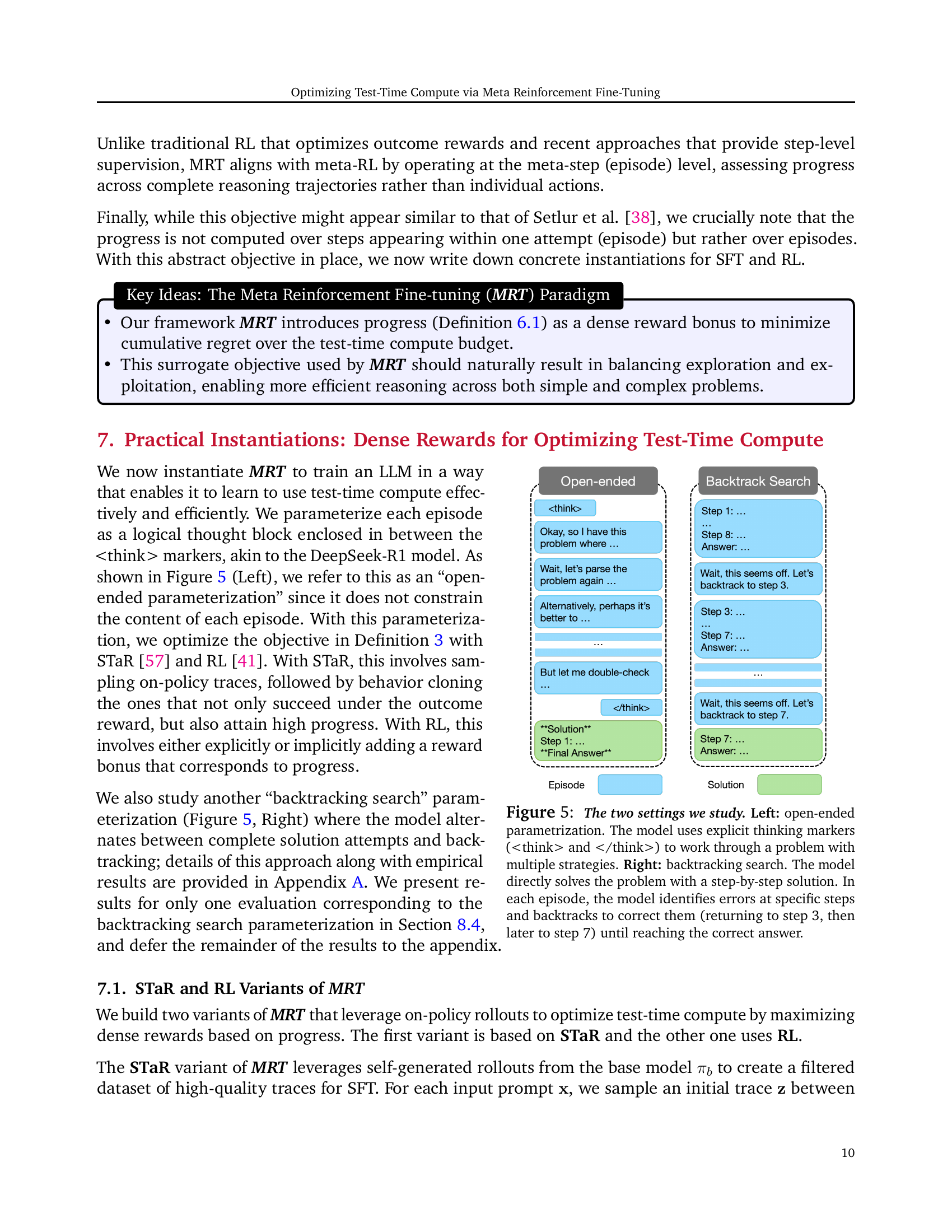
🔼 This figure illustrates two different approaches to prompting LLMs for complex reasoning tasks. The left panel depicts the ‘open-ended parametrization’, where the model uses explicit thinking markers (
and ) to explore multiple solution strategies within a given reasoning chain. The model is free to make progress or regress. The right panel shows the ‘backtracking search’ approach. Here, the model directly tackles the problem step-by-step. Importantly, each episode involves error detection; if an error is found, the model backtracks to a previous step to correct the mistake before proceeding further, effectively refining its solution iteratively.read the caption
Figure 5: The two settings we study. Left: open-ended parametrization. The model uses explicit thinking markers (and ) to work through a problem with multiple strategies. Right: backtracking search. The model directly solves the problem with a step-by-step solution. In each episode, the model identifies errors at specific steps and backtracks to correct them (returning to step 3, then later to step 7) until reaching the correct answer.

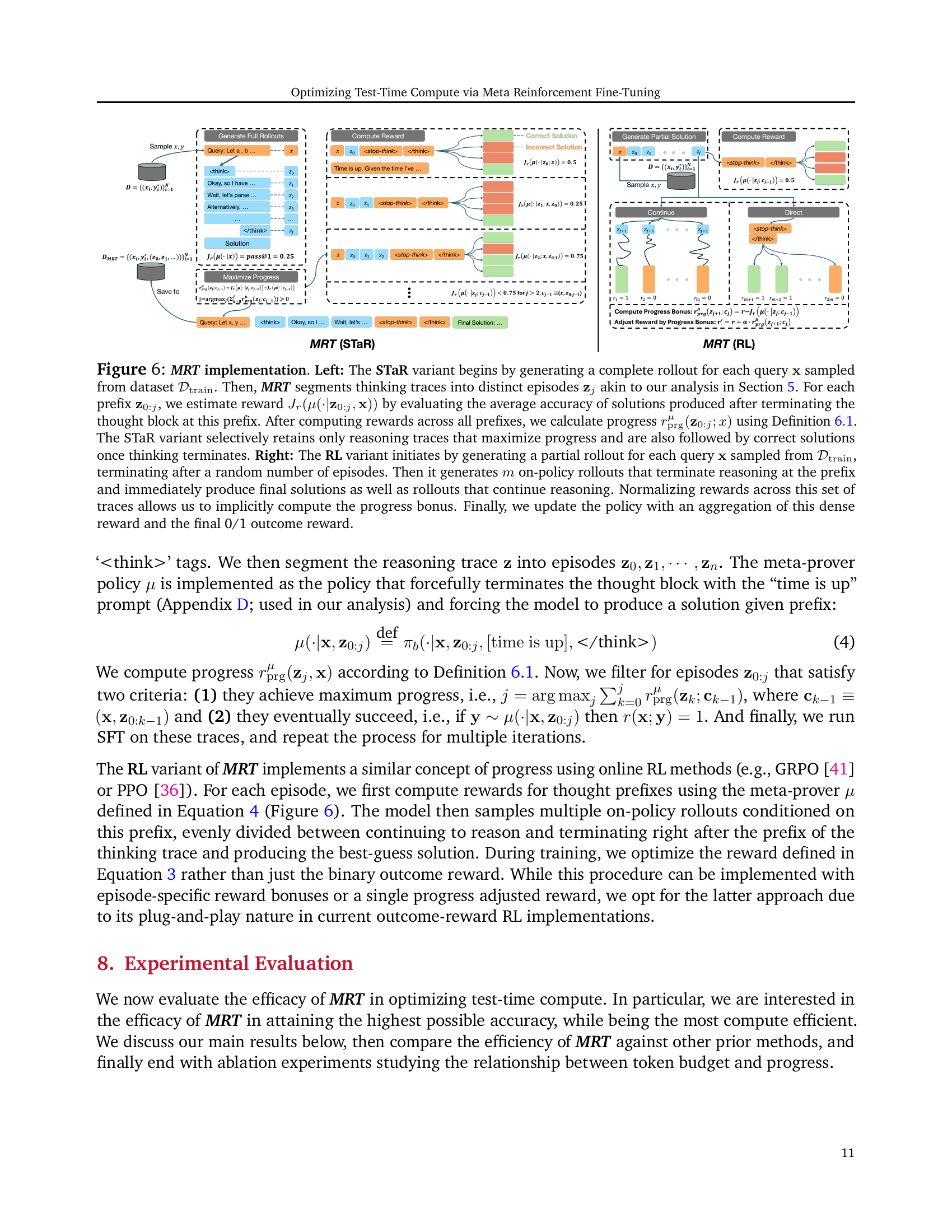
🔼 This figure illustrates the implementation details of the Meta Reinforcement Fine-Tuning (MRT) algorithm. The left panel shows the STaR (Successor-based Reinforcement Learning) variant, which starts by generating a complete reasoning trace for each problem. This trace is then divided into episodes, and a reward is calculated based on the progress made in each episode toward a correct solution, using the progress metric defined in Definition 6.1. Only traces that maximize progress and lead to a correct solution are kept. The right panel shows the RL (Reinforcement Learning) variant. Here, partial rollouts are generated, and multiple additional rollouts are simulated: some that stop at the partial rollout and produce a final answer, and some that continue reasoning. The rewards are normalized, implicitly calculating a progress bonus, and the policy is updated using both the progress reward and the final 0/1 outcome reward.
read the caption
Figure 6: MRT implementation. Left: The STaR variant begins by generating a complete rollout for each query 𝐱𝐱\mathbf{x}bold_x sampled from dataset 𝒟trainsubscript𝒟train\mathcal{D}_{\mathrm{train}}caligraphic_D start_POSTSUBSCRIPT roman_train end_POSTSUBSCRIPT. Then, MRT segments thinking traces into distinct episodes 𝐳jsubscript𝐳𝑗\mathbf{z}_{j}bold_z start_POSTSUBSCRIPT italic_j end_POSTSUBSCRIPT akin to our analysis in Section 5. For each prefix 𝐳0:jsubscript𝐳:0𝑗\mathbf{z}_{0:j}bold_z start_POSTSUBSCRIPT 0 : italic_j end_POSTSUBSCRIPT, we estimate reward Jr(μ(⋅|𝐳0:j,𝐱))J_{r}(\mu(\cdot|\mathbf{z}_{0:j},\mathbf{x}))italic_J start_POSTSUBSCRIPT italic_r end_POSTSUBSCRIPT ( italic_μ ( ⋅ | bold_z start_POSTSUBSCRIPT 0 : italic_j end_POSTSUBSCRIPT , bold_x ) ) by evaluating the average accuracy of solutions produced after terminating the thought block at this prefix. After computing rewards across all prefixes, we calculate progress rprgμ(𝐳0:j;x)subscriptsuperscript𝑟𝜇prgsubscript𝐳:0𝑗𝑥r^{\mu}_{\mathrm{prg}}(\mathbf{z}_{0:j};x)italic_r start_POSTSUPERSCRIPT italic_μ end_POSTSUPERSCRIPT start_POSTSUBSCRIPT roman_prg end_POSTSUBSCRIPT ( bold_z start_POSTSUBSCRIPT 0 : italic_j end_POSTSUBSCRIPT ; italic_x ) using Definition 6.1. The STaR variant selectively retains only reasoning traces that maximize progress and are also followed by correct solutions once thinking terminates. Right: The RL variant initiates by generating a partial rollout for each query 𝐱𝐱\mathbf{x}bold_x sampled from 𝒟trainsubscript𝒟train\mathcal{D}_{\mathrm{train}}caligraphic_D start_POSTSUBSCRIPT roman_train end_POSTSUBSCRIPT, terminating after a random number of episodes. Then it generates m𝑚mitalic_m on-policy rollouts that terminate reasoning at the prefix and immediately produce final solutions as well as rollouts that continue reasoning. Normalizing rewards across this set of traces allows us to implicitly compute the progress bonus. Finally, we update the policy with an aggregation of this dense reward and the final 0/1 outcome reward.

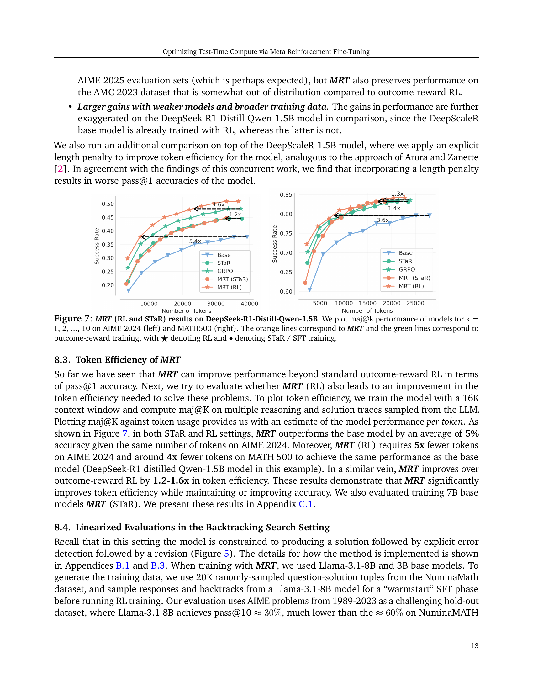
🔼 Figure 7 displays the results of applying Meta Reinforcement Fine-tuning (MRT) using both reinforcement learning (RL) and self-training with reinforcement (STaR) to the DeepSeek-R1-Distill-Qwen-1.5B language model. The performance metric used is maj@k, which represents the majority vote accuracy across k independent attempts at solving problems. The plots show maj@k performance for k values ranging from 1 to 10 on two different benchmarks: AIME 2024 (left panel) and MATH500 (right panel). Orange lines represent the performance achieved with MRT, while green lines depict the results using standard outcome-reward training methods. Within each panel, solid lines represent RL results, and dashed lines denote the STaR/SFT results. This figure directly illustrates MRT’s effectiveness in improving accuracy and token efficiency compared to traditional outcome-reward training.
read the caption
Figure 7: MRT (RL and STaR) results on DeepSeek-R1-Distill-Qwen-1.5B. We plot maj@k performance of models for k = 1, 2, …, 10 on AIME 2024 (left) and MATH500 (right). The orange lines correspond to MRT and the green lines correspond to outcome-reward training, with ★★\bigstar★ denoting RL and ∙∙\bullet∙ denoting STaR / SFT training.

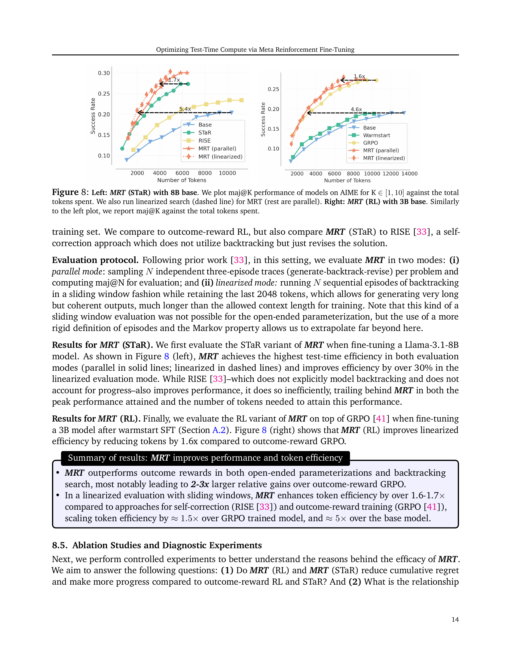
🔼 This figure compares the performance of different models on the AIME benchmark. The left panel shows the results for the MRT (STaR) model with an 8B base, illustrating how its performance (maj@K) changes with increasing token usage, comparing parallel and linearized search methods. The right panel presents similar results for the MRT (RL) model with a 3B base. This figure visually demonstrates the trade-off between model accuracy and computational cost for various models and search strategies.
read the caption
Figure 8: Left: MRT (STaR) with 8B base. We plot maj@K performance of models on AIME for K ∈[1,10]absent110\in[1,10]∈ [ 1 , 10 ] against the total tokens spent. We also run linearized search (dashed line) for MRT (rest are parallel). Right: MRT (RL) with 3B base. Similarly to the left plot, we report maj@K against the total tokens spent.

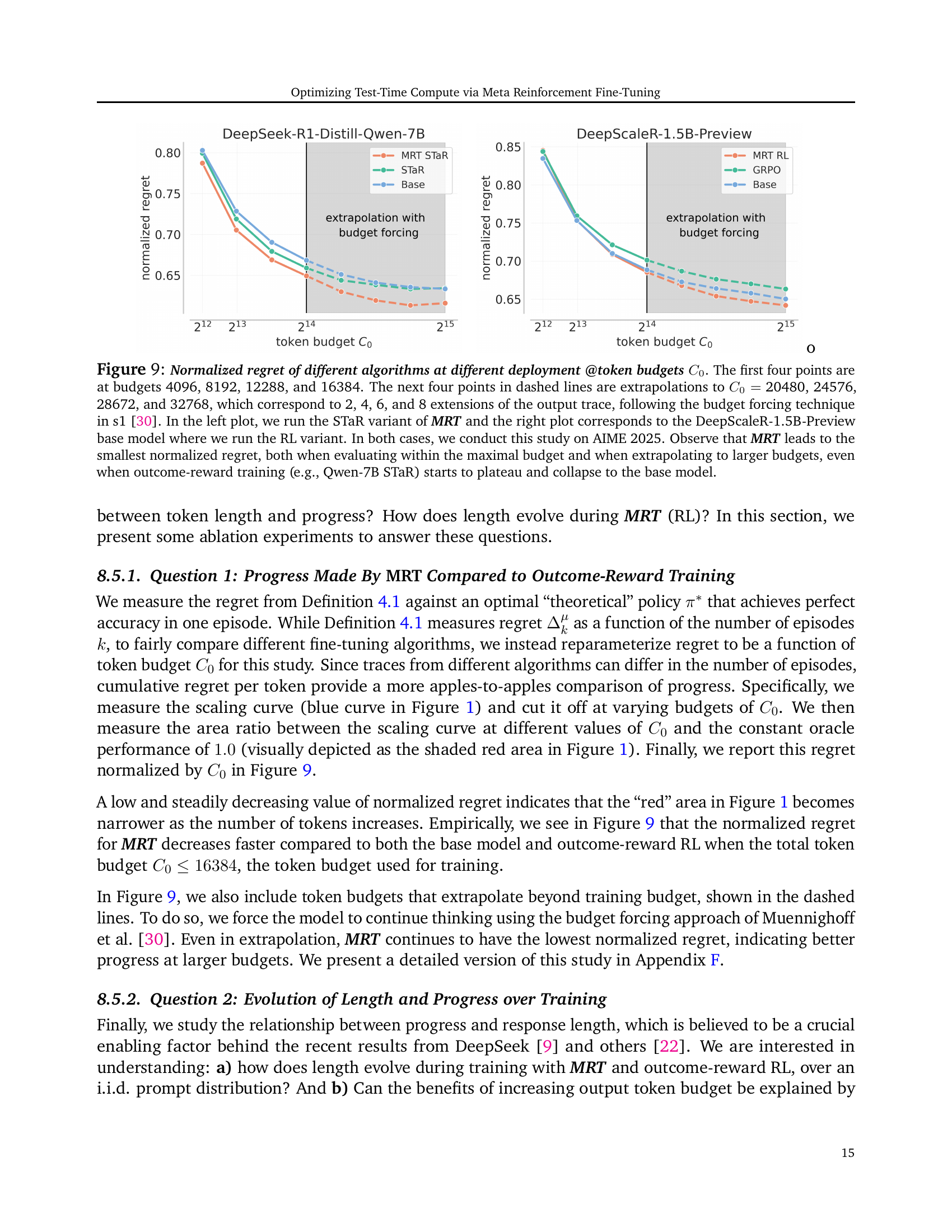
🔼 Figure 9 presents a comparison of cumulative regret, a measure of the efficiency of test-time compute, across different algorithms at varying token budgets. The x-axis represents the token budget (C0), while the y-axis shows the normalized cumulative regret. The solid points show results for budgets of 4096, 8192, 12288, and 16384 tokens. The dashed lines extrapolate these results to larger budgets (20480, 24576, 28672, and 32768 tokens), simulating the effect of extending the model’s reasoning process using a ‘budget forcing’ technique. The left plot uses the STaR variant of the MRT method and the DeepSeek-R1-Distill-Qwen-7B model; the right plot uses the RL variant of MRT with the DeepScaleR-1.5B-Preview model. Both plots show results for AIME 2025 problems. The figure demonstrates that MRT consistently achieves lower cumulative regret than other methods, both within the initial budget range and when extrapolated to higher budgets, highlighting its superior efficiency in utilizing test-time computational resources. The figure illustrates that outcome-reward baselines (e.g., Qwen-7B STaR) eventually stagnate, whereas MRT continues to show improvement.
read the caption
Figure 9: Normalized regret of different algorithms at different deployment @token budgets C0subscriptC0C_{0}italic_C start_POSTSUBSCRIPT 0 end_POSTSUBSCRIPT. The first four points are at budgets 4096, 8192, 12288, and 16384. The next four points in dashed lines are extrapolations to C0=subscript𝐶0absentC_{0}=italic_C start_POSTSUBSCRIPT 0 end_POSTSUBSCRIPT = 20480, 24576, 28672, and 32768, which correspond to 2, 4, 6, and 8 extensions of the output trace, following the budget forcing technique in s1 [30]. In the left plot, we run the STaR variant of MRT and the right plot corresponds to the DeepScaleR-1.5B-Preview base model where we run the RL variant. In both cases, we conduct this study on AIME 2025. Observe that MRT leads to the smallest normalized regret, both when evaluating within the maximal budget and when extrapolating to larger budgets, even when outcome-reward training (e.g., Qwen-7B STaR) starts to plateau and collapse to the base model.

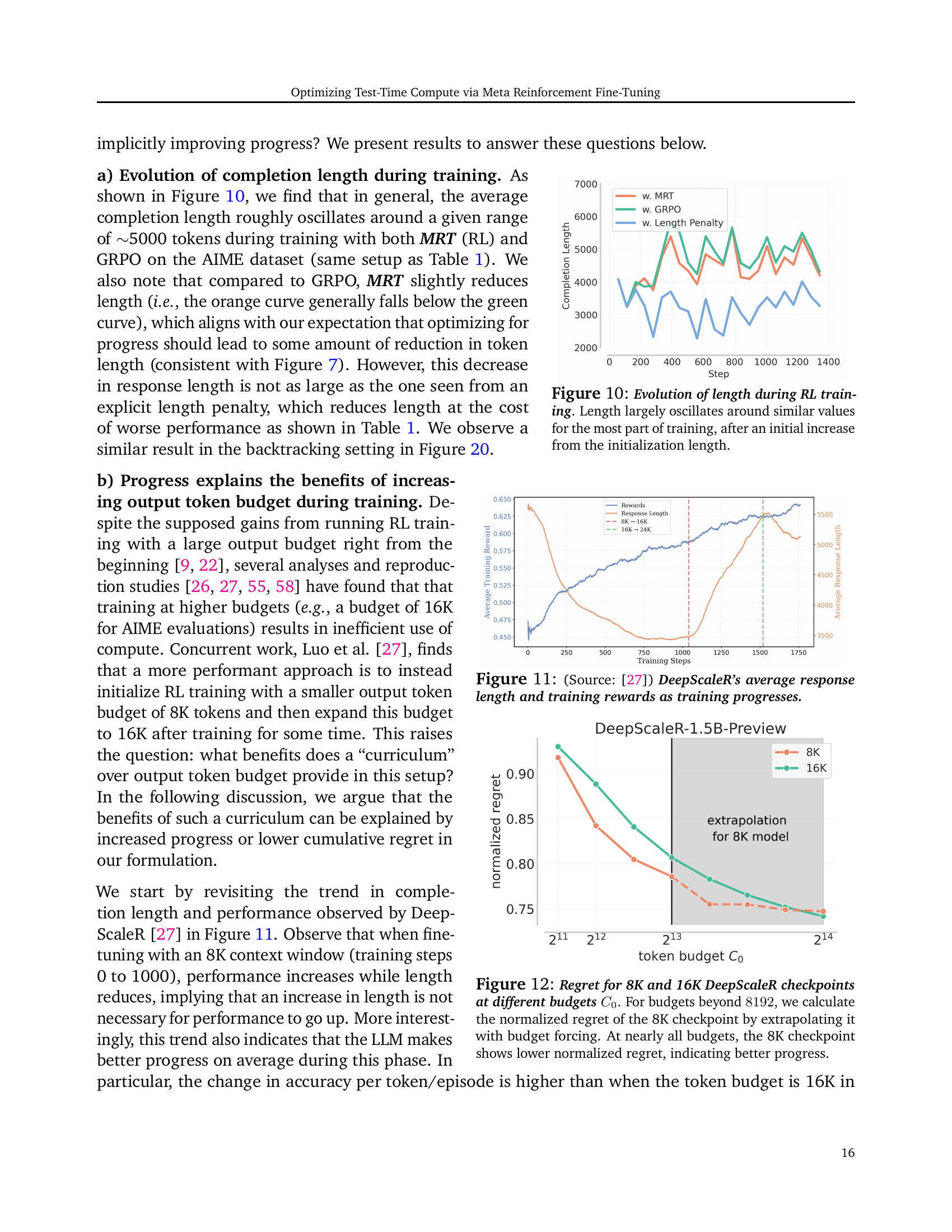
🔼 This figure shows the evolution of the average response length during the reinforcement learning (RL) training process. Initially, there is a noticeable increase in the average length. However, for the majority of the training, the length oscillates around a relatively stable mean value. This suggests that while the model initially explores longer response sequences, it eventually settles into a more consistent pattern of generating responses of similar lengths.
read the caption
Figure 10: Evolution of length during RL training. Length largely oscillates around similar values for the most part of training, after an initial increase from the initialization length.

🔼 This figure, sourced from Luo et al. [27], illustrates the trends in average response length and training rewards observed during the DeepScaleR model’s training process. It shows how these two metrics evolve over the course of training, providing insights into the model’s learning dynamics and its relationship between length of responses and training effectiveness.
read the caption
Figure 11: (Source: [27]) DeepScaleR’s average response length and training rewards as training progresses.

🔼 Figure 12 illustrates the cumulative regret (a measure of how well an LLM uses its compute budget) for two different training scenarios: one with an 8K token budget and another with a 16K token budget. The graph shows that even when extrapolating the 8K model’s performance to higher budgets (using a technique called ‘budget forcing’), the 8K model consistently exhibits lower cumulative regret. This suggests that the 8K model makes more efficient and effective use of its compute resources, demonstrating better progress towards solving problems.
read the caption
Figure 12: Regret for 8K and 16K DeepScaleR checkpoints at different budgets C0subscriptC0C_{0}italic_C start_POSTSUBSCRIPT 0 end_POSTSUBSCRIPT. For budgets beyond 8192819281928192, we calculate the normalized regret of the 8K checkpoint by extrapolating it with budget forcing. At nearly all budgets, the 8K checkpoint shows lower normalized regret, indicating better progress.

🔼 This figure illustrates the process of on-policy rollout generation within the MRT framework for the backtracking search setting. The model starts with an initial response (z0). It then generates a backtracking episode (z1) where it identifies errors in z0. Finally, it produces a corrected response (z2). Importantly, the reward is adjusted based on the progress made toward a correct solution, encouraging the model to effectively utilize backtracking for improved accuracy. The progress is measured as a change in the likelihood of eventual success between consecutive steps.
read the caption
Figure 13: On-policy rollout generation for MRT in the backtracking search setting. MRT allows the model to learn to backtrack (𝐳1subscript𝐳1\mathbf{z}_{1}bold_z start_POSTSUBSCRIPT 1 end_POSTSUBSCRIPT) and generate the corrected attempt (𝐳2subscript𝐳2\mathbf{z}_{2}bold_z start_POSTSUBSCRIPT 2 end_POSTSUBSCRIPT) with a progress-adjusted reward.

🔼 This figure illustrates different methods for creating training data to enable a language model to perform backtracking. The standard approach (RISE) involves creating training examples by stitching together a successful reasoning trace with some failures. The MRT approach improves on this by explicitly modeling backtracking within the training data, which allows it to better learn how to effectively use backtracking during test-time reasoning. In the MRT approach, the algorithm traverses two paths, which share the same prefix and then uses a backtracking step to reach a correct answer. This method focuses on using backtracking to improve reasoning capabilities, instead of just training the model to recognize solutions.
read the caption
Figure 14: Different data construction schemes for obtaining warmstart SFT data for the backtracking search setting. MRT traverses two paths with the shared prefix, making use of backtracking, which RISE style approaches.

🔼 This figure displays the training loss curves for three different methods used to prepare training data for a model using backtracking search. The three methods are: 1. Random stitching (RISE): This method combines random parts of incorrect solution attempts and correct solutions to create training examples. 2. Rejection sampling (STaR): This method uses a sampling technique to select a subset of high-quality solution traces from many generated traces to create training examples. 3. Backtracking: This method, proposed by the authors, employs a more structured process to create training data based on identified errors and subsequent corrections in the model’s solution attempts. The lower the training loss, the easier it is for the model to learn from the training data created by that method. This experiment shows that the backtracking approach is better, having the lowest loss, followed by the STaR approach. The random stitching approach resulted in the highest training loss, implying the training data it produced is the most difficult for the model to learn from.
read the caption
Figure 15: Training loss for warmstart SFT on multiple data configurations: random stitching (“RISE” [33]), STaR (“rejection sampling”), and our warmstart SFT data (“Backtrack”). A lower loss implies ease of fitting this data.
🔼 This figure presents histograms that compare the progress made during backtracking episodes by different training methods: RISE, MRT (STaR), GRPO, and MRT (RL). The x-axis represents the difference between the backtracking reward and the direct reward. The y-axis represents the frequency of these reward differences. Each histogram illustrates the distribution of progress values calculated during backtracking episodes. The results show that MRT (both STaR and RL variants) consistently achieves higher progress values compared to RISE and GRPO, indicating a more effective strategy in utilizing test-time compute to make consistent progress towards a solution.
read the caption
Figure 16: Progress histograms in the backtracking search setting over the backtracking episode for RISE and MRT (STaR) on the left and GRPO and MRT (RL) on right, computed on the evaluation set. In each case, using reward values prescribed by MRT amplifies information gain on the test-time trace, enabling it to make consistent progress.
More on tables
| Hyperparameter | Values |
|---|---|
| learning_rate | 1.0e-6 |
| num_train_epochs | 3 |
| batch_size | 256 |
| gradient_checkpointing | True |
| max_seq_length | 16384 |
| bf16 | True |
| num_gpus | 8 |
| learning rate | 1e-6 |
| warmup ratio | 0.1 |
🔼 This table lists the hyperparameters used for training the Meta Reinforcement Fine-Tuning (MRT) model using the STaR (self-training with rejection sampling) algorithm. It includes values for parameters such as the learning rate, the number of training epochs, batch size, gradient checkpointing setting, maximum sequence length, whether bf16 precision is used, and the number of GPUs used for training. The learning rate schedule’s warmup ratio is also specified.
read the caption
Table 2: Hyperparameters used for MRT (STaR)
| Hyperparameter | Values |
|---|---|
| learning_rate | 1.0e-6 |
| lr_scheduler_type | cosine |
| warmup_ratio | 0.1 |
| weight_decay | 0.01 |
| num_train_epochs | 1 |
| batch_size | 256 |
| max_prompt_length | 4096 |
| max_completion_length | 24576 |
| num_generations | 4 |
| use_vllm | True |
| vllm_gpu_memory_utilization | 0.8 |
| temperature | 0.9 |
| bf16 | True |
| num_gpus | 8 |
| deepspeed_multinode_launcher | standard |
| zero3_init_flag | true |
| zero_stage | 3 |
🔼 This table lists the hyperparameters used during the training process of the Meta Reinforcement Fine-Tuning (MRT) method using the Reinforcement Learning (RL) approach. The hyperparameters control various aspects of the training process, influencing factors like the learning rate, batch size, network architecture, and optimization algorithm. These settings are crucial in achieving optimal performance and efficiency during the model training.
read the caption
Table 3: Hyperparameters used for MRT (RL)
| Hyperparameter | Values |
|---|---|
| learning_rate | 1.0e-6 |
| num_train_epochs | 3 |
| batch_size | 256 |
| gradient_checkpointing | True |
| max_seq_length | 4096 |
| bf16 | True |
| num_gpus | 8 |
| learning rate | 1e-6 |
| warmup ratio | 0.1 |
🔼 This table lists the hyperparameters used for training the Meta Reinforcement Fine-Tuning (MRT) model using the STaR algorithm. It includes settings for the learning rate, number of training epochs, batch size, gradient checkpointing, maximum sequence length, use of bf16 precision, number of GPUs used for training, and the learning rate warmup ratio. These hyperparameters were specifically tuned for the experiments using the STaR approach within the MRT framework.
read the caption
Table 4: Hyperparameters used for MRT (STaR)
| Hyperparameter | Values |
|---|---|
| learning_rate | 1.0e-6 |
| lr_scheduler_type | cosine |
| warmup_ratio | 0.1 |
| weight_decay | 0.01 |
| num_train_epochs | 1 |
| batch_size | 256 |
| max_prompt_length | 1500 |
| max_completion_length | 1024 |
| num_generations | 4 |
| use_vllm | True |
| vllm_gpu_memory_utilization | 0.8 |
| temperature | 0.9 |
| bf16 | True |
| num_gpus | 8 |
| deepspeed_multinode_launcher | standard |
| zero3_init_flag | true |
| zero_stage | 3 |
🔼 This table lists the hyperparameters used for training language models using the Meta Reinforcement Fine-Tuning (MRT) paradigm with reinforcement learning (RL). It details the specific settings used for the learning rate, scheduler type, weight decay, number of training epochs, batch size, maximum prompt and completion lengths, number of generations, use of the vllm library, GPU memory utilization settings, temperature, use of bf16 precision, number of GPUs, deepspeed multinode launcher settings, and zero stage settings. These hyperparameters are crucial for optimizing the performance and efficiency of test-time computation within the MRT-RL framework.
read the caption
Table 5: Hyperparameters used for MRT (RL)
Full paper#