TL;DR#
Large Language Models (LLMs) are powerful but computationally expensive, making them difficult to deploy in resource-constrained environments. Existing pruning methods often apply a uniform sparsity pattern across all tasks, potentially overlooking task-dependent knowledge representations. To solve these issues, this paper presents the intruiging parallel of cognitive neuroscience and conventional pruning approaches. Different tasks rely on distinct sets of neurons working collaboratively, a dynamic, task-aware strategy is needed for LLMs.
This paper introduces Sparse Expert Activation Pruning (SEAP), a training-free pruning method that selectively retains task-relevant parameters to reduce inference overhead. SEAP identifies task-specific expert activation patterns and prunes the model while preserving task performance and enhancing computational efficiency. Experiments demonstrate that SEAP significantly reduces computational overhead while maintaining competitive accuracy. SEAP surpasses both WandA and FLAP by over 20% at 50% pruning and only incurs a 2.2% performance drop compared to the dense model at 20% pruning.
Key Takeaways#
Why does it matter?#
This paper introduces a novel training-free pruning method that dynamically adapts to task-specific activation patterns, offering a promising approach to optimize LLMs for real-world applications and paving the way for future advancements in structured pruning.
Visual Insights#

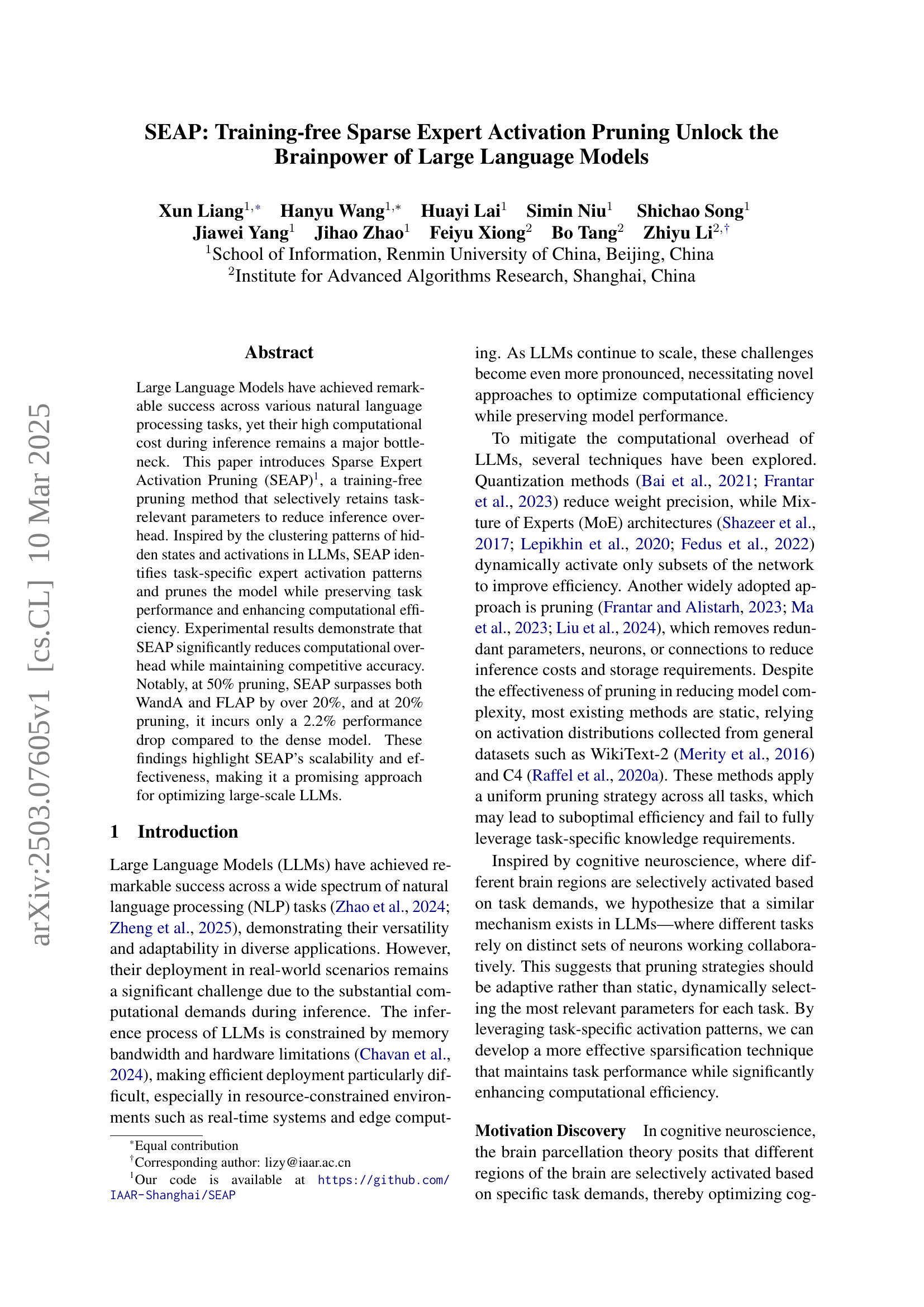
🔼 This figure visualizes the activation patterns of hidden states within a large language model (LLM) across various tasks. Each point represents a specific hidden state’s activation level for a particular task. The x and y coordinates represent the dimensionality reduction of the high-dimensional hidden states. Crucially, the plot reveals distinct clusters of points corresponding to different task categories. Tasks with similar semantic or reasoning requirements tend to cluster together, indicating that these tasks activate similar regions within the LLM’s hidden state space. This supports the hypothesis that the LLM’s internal representations for various tasks are not uniformly distributed but are instead organized in task-specific clusters. This observation is fundamental to the paper’s proposed method.
read the caption
Figure 1: Visualization of hidden states h(P)ℎ𝑃h(P)italic_h ( italic_P ) from different tasks. Each point represents the activation of a hidden state in the model for a specific task. The clustering patterns illustrate how tasks with similar requirements tend to activate similar regions in the model.
| Pruning Ratio | Method | Llama-2-7B | |||||||
|---|---|---|---|---|---|---|---|---|---|
| WinoGrande | OBQA | HellaSwag | PIQA | ARC-c | ARC-e | BoolQ | Average | ||
| 0% | Dense | 69.14 | 44.20 | 76.01 | 79.11 | 46.33 | 76.26 | 77.71 | 66.97 |
| 20% | WandA-sp () | 62.67 | 40.80 | 71.56 | 76.28 | 42.41 | 71.93 | 61.01 | 60.95 |
| SEAP () | 66.77 | 43.00 | 72.53 | 77.80 | 45.48 | 75.42 | \ul71.77 | 64.68 | |
| SEAP-gen () | \ul67.80 | 41.00 | 73.77 | 77.58 | 44.71 | \ul74.33 | 71.44 | 64.38 | |
| FLAP () | 67.32 | 41.00 | 72.77 | 76.12 | 42.75 | 71.93 | 62.57 | 62.07 | |
| SEAP () | 68.19 | \ul42.60 | \ul74.07 | \ul78.07 | \ul45.39 | 75.42 | 74.50 | 65.46 | |
| SEAP-gen () | 67.72 | 41.20 | 74.82 | 78.35 | \ul45.39 | 74.12 | 71.68 | \ul64.75 | |
| 50% | WandA-sp () | 52.72 | 35.20 | 41.11 | 64.36 | 30.97 | 52.78 | 39.45 | 45.23 |
| SEAP () | 56.12 | 37.20 | 58.07 | \ul73.83 | 38.74 | 61.32 | 60.15 | \ul55.06 | |
| SEAP-gen () | 54.70 | 38.20 | 56.97 | 71.76 | 35.24 | 57.15 | 57.25 | 53.04 | |
| FLAP () | 56.04 | 34.40 | 48.62 | 63.00 | 32.17 | 51.18 | 42.32 | 46.82 | |
| SEAP () | 60.14 | \ul38.80 | 58.22 | 74.32 | \ul38.14 | \ul60.56 | \ul59.94 | 55.73 | |
| SEAP-gen () | \ul59.91 | 39.80 | \ul58.17 | 73.39 | 37.97 | 55.72 | 57.98 | 54.71 | |
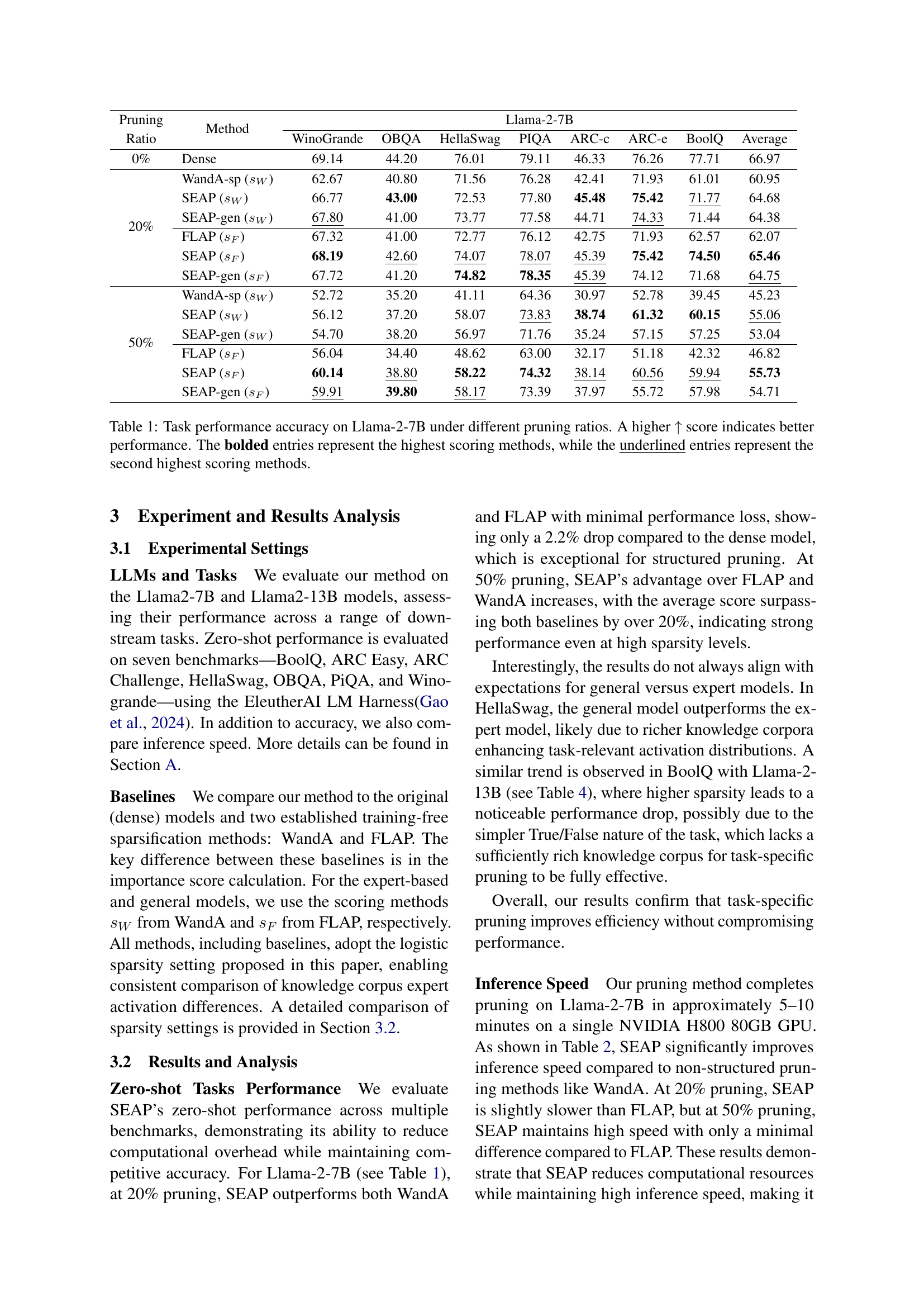
🔼 This table presents the results of the SEAP model’s performance on the Llama-2-7B model across various downstream tasks. It compares the accuracy of the model under different pruning ratios (0%, 20%, and 50%), showing the impact of the proposed SEAP method, as well as the FLAP and WandA baselines. The table shows accuracy scores for each task, allowing for a comparison of the different methods’ performance across various sparsity levels. The bolded scores represent the highest performing method for a given task and pruning ratio, while underlined scores indicate the second highest.
read the caption
Table 1: Task performance accuracy on Llama-2-7B under different pruning ratios. A higher ↑ score indicates better performance. The bolded entries represent the highest scoring methods, while the underlined entries represent the second highest scoring methods.
In-depth insights#
Brainpower LLM#
The concept of a “Brainpower LLM” evokes the idea of an LLM optimized for both performance and efficiency. This necessitates a delicate balance, moving beyond simply scaling model size to achieve higher accuracy. Efficient resource utilization becomes paramount, focusing on strategies like pruning, quantization, and knowledge distillation to reduce computational overhead. A true Brainpower LLM likely incorporates task-specific optimization techniques, dynamically allocating resources based on the demands of the input. This could involve selectively activating network components or utilizing specialized modules for certain tasks. Adaptive learning and continual refinement are also crucial aspects. By analyzing patterns in data and user interactions, the model can identify areas for improvement and fine-tune its parameters to enhance both accuracy and efficiency, solidifying its spot as a genuine Brainpower LLM.
Task-Spec Pruning#
Task-specific pruning offers a promising avenue for optimizing large language models (LLMs) by tailoring the model’s architecture to the demands of individual tasks. Instead of applying a uniform pruning strategy across all tasks, this approach selectively removes parameters that are deemed less relevant for a particular task, preserving the parameters crucial for optimal performance. This strategy leverages the observation that different tasks activate distinct sets of neurons within LLMs. Adaptively retain the most relevant parameters based on the task’s specific characteristics, enhancing computational efficiency while preserving task performance. This approach directly addresses the heterogeneity of tasks and the redundancy of a one-size-fits-all model. By carefully sculpting the model to fit the contours of each task, this can lead to more efficient use of computational resources and improved performance. It makes the models more scalable and adaptive.
Activat. Patterns#
Analyzing activation patterns in LLMs is crucial for understanding how these models process information. By examining which neurons and layers are activated for specific tasks, we can gain insights into task-specific knowledge representations. This understanding can lead to more efficient pruning strategies, dynamically retaining only the most relevant parameters. Exploring the activation landscape allows for adaptive sparsification, optimizing computational efficiency while preserving performance. Ultimately, understanding these patterns leads to specialized LLM deployment and efficient performance.
Sparsity Setting#
The research employs a sparsity setting to strategically determine which neurons to prune in LLMs. The study conducts a remove test on MMLU and PIQA, analyzing performance at different sparsity levels, showing early layers are more sensitive to pruning, while deeper layers tolerate higher sparsity with minimal loss. Inspired by LLM-Pruner and FLAP, sparsity of the final layers is set to zero, adjusting sparsity of other layers to maintain overall sparsity. The research uses a differentiable logistic function for a smooth sparsity distribution across layers, ensuring lower sparsity in early layers and higher sparsity in deeper layers. The global sparsity target is met through numerical search for A. This approach allows for more efficient resource allocation and better performance, as confirmed by results surpassing WandA and FLAP.
Efficient LLMs#
Efficient LLMs are crucial for wider accessibility and deployment, addressing limitations in memory bandwidth and hardware. Techniques such as quantization reduce weight precision, while pruning removes redundant parameters. Methods like MoE dynamically activate subsets of the network. Task-specific knowledge can enhance sparsification techniques which adaptively retain parameters, enhancing performance. There is an emerging trend of activation pruning, which reduces memory bandwidth during inference by sparsifying network activations. Balancing efficiency and performance requires adaptive sparsity strategies, ensuring critical neurons are retained, optimizing resource allocation, and better performance, highlighting potential for practical applications.
More visual insights#
More on figures

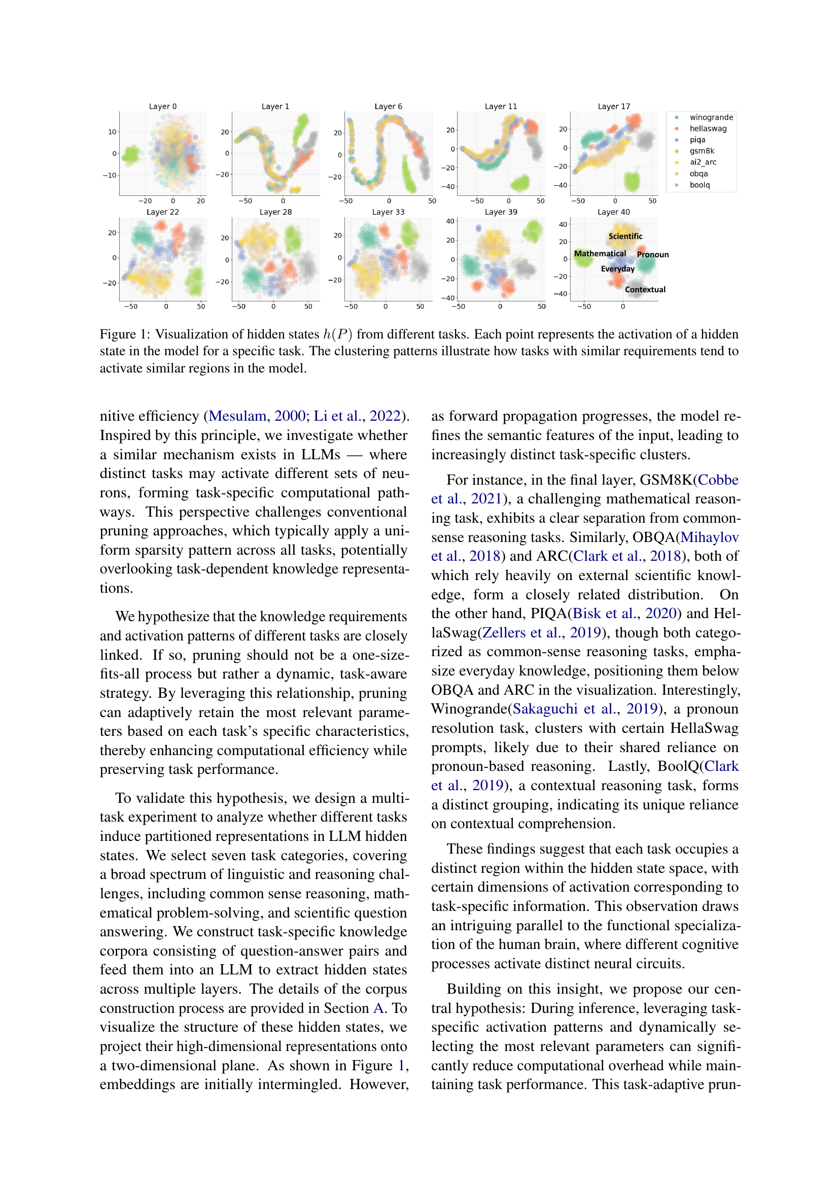
🔼 This figure provides a detailed overview of the SEAP (Sparse Expert Activation Pruning) approach. The left side focuses on the ‘Motivation Discovery’ phase, illustrating how task-specific activation patterns are identified. This is achieved by analyzing the hidden states and neuron activations extracted from a carefully constructed task corpus. The right side of the figure details the five main steps involved in the ‘Training-free Sparse Expert Activation Pruning’ process itself, as described in Section 2.1 of the paper. Each step is shown visually to clarify the process of pruning based on task-specific activation patterns.
read the caption
Figure 2: Framework of the SEAP approach. The left side shows the Motivation Discovery phase, where task-specific activation patterns are identified by analyzing hidden states and neuron activations extracted from the task corpus. The right side illustrates the Training-free Sparse Expert Activation Pruning process, consisting of five main steps described in Section 2.1.

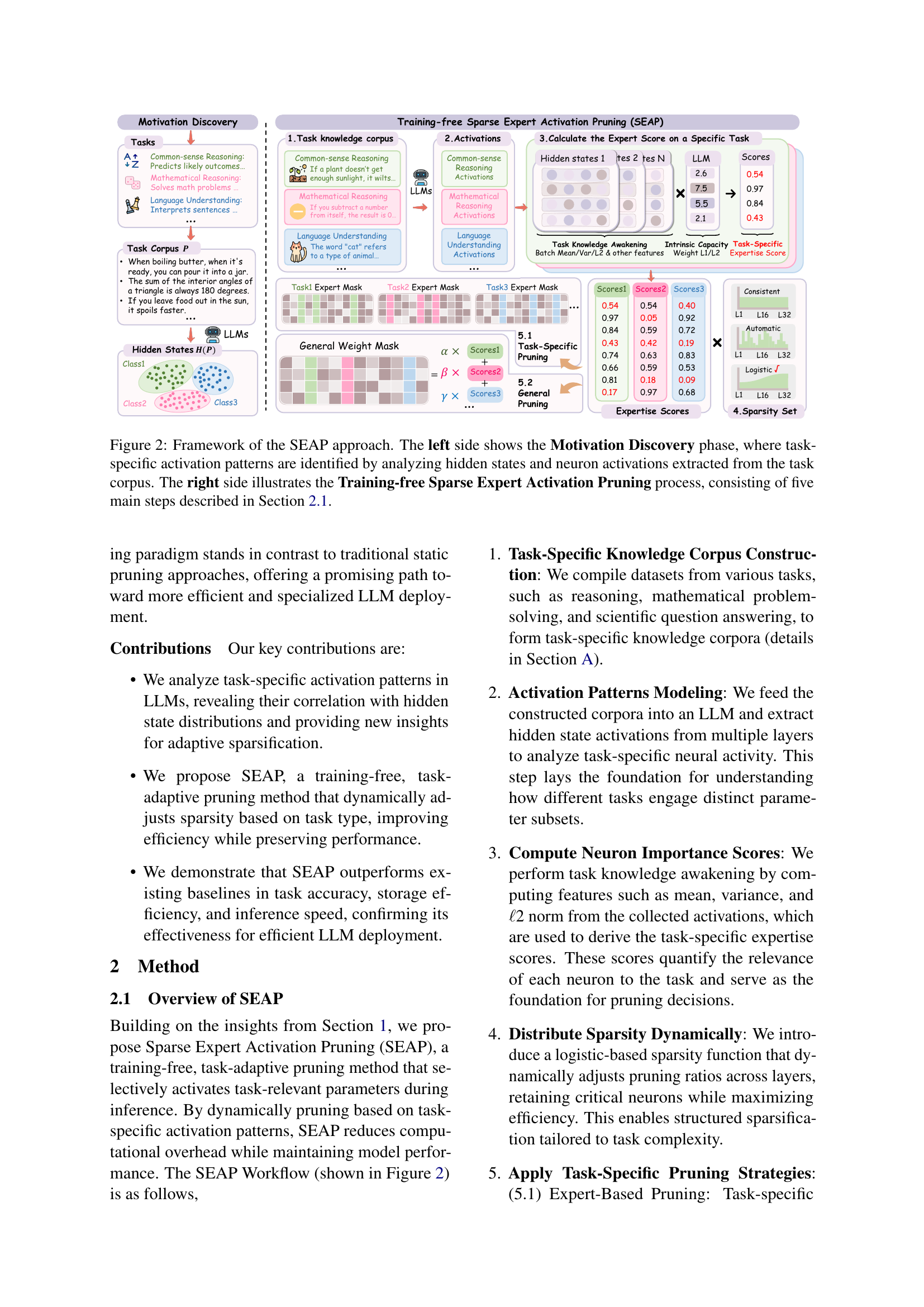
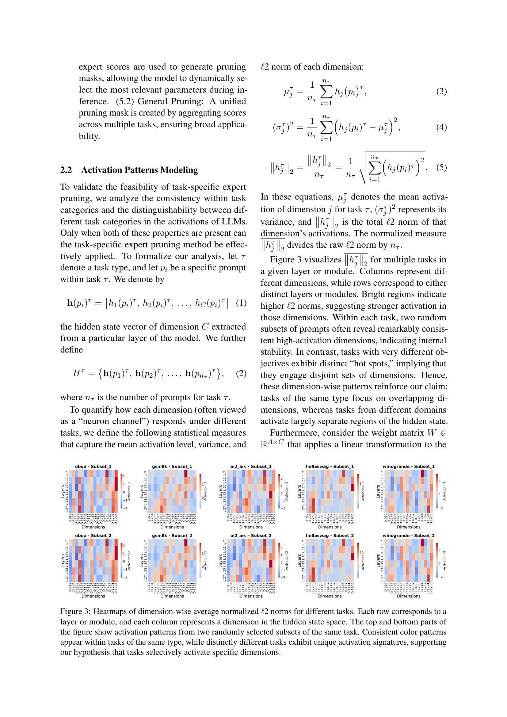
🔼 This figure visualizes the activation patterns of different tasks within a language model. Heatmaps display the average ℓ2 norm of each dimension in the hidden state across multiple layers or modules. Each row represents a layer/module, and each column represents a dimension. The top and bottom halves of each heatmap show activation patterns from two different, randomly selected subsets of prompts from the same task. Consistent color patterns within each task’s heatmaps illustrate that similar tasks activate similar dimensions, while distinctly different tasks show unique activation patterns. This supports the study’s hypothesis that tasks selectively activate specific dimensions of the hidden state.
read the caption
Figure 3: Heatmaps of dimension-wise average normalized ℓℓ\ellroman_ℓ2 norms for different tasks. Each row corresponds to a layer or module, and each column represents a dimension in the hidden state space. The top and bottom parts of the figure show activation patterns from two randomly selected subsets of the same task. Consistent color patterns appear within tasks of the same type, while distinctly different tasks exhibit unique activation signatures, supporting our hypothesis that tasks selectively activate specific dimensions.

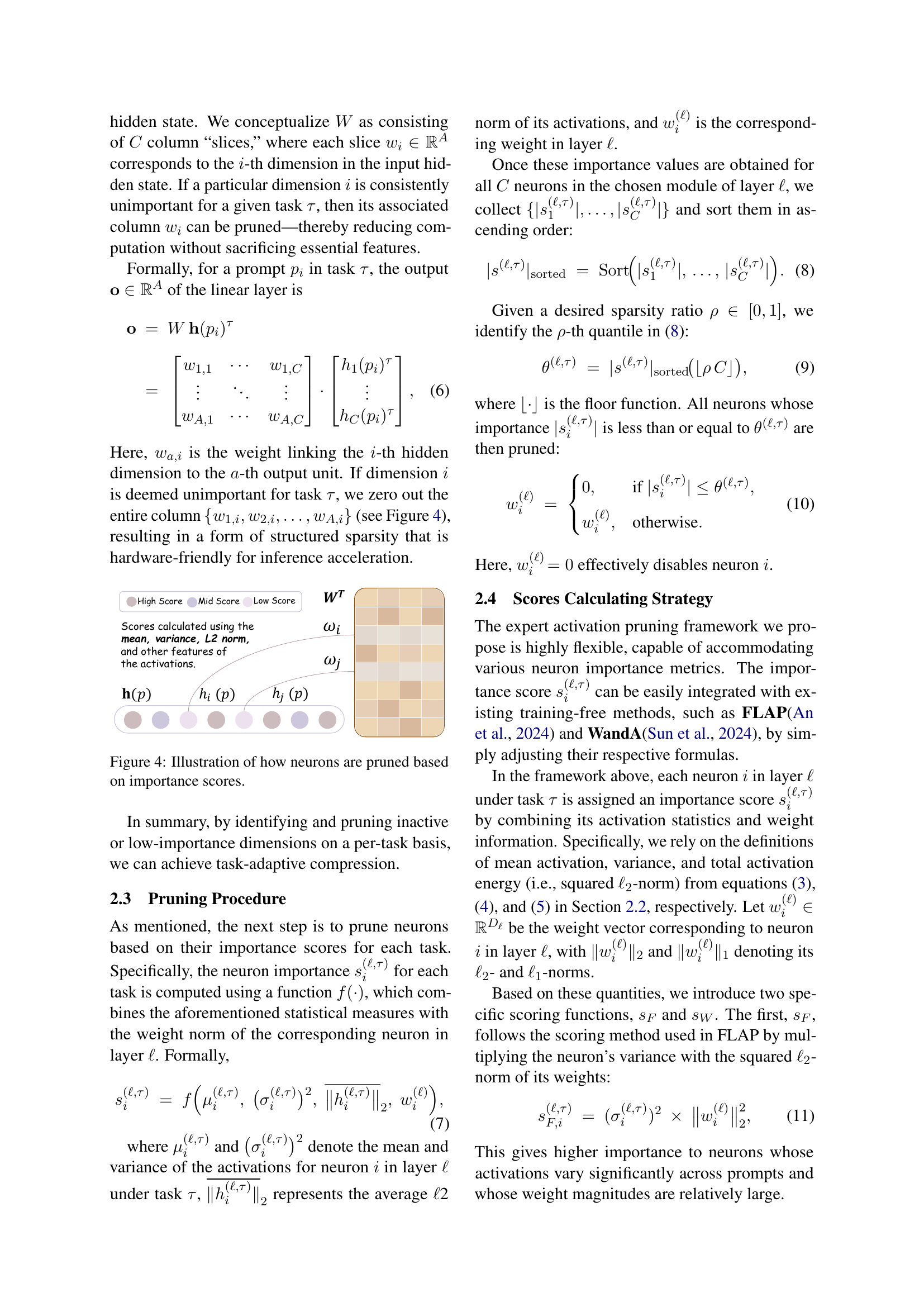
🔼 This figure illustrates the process of neuron pruning in SEAP. Neurons with low importance scores (indicated by color) are pruned, while those with high scores are retained. This selective pruning enhances computational efficiency while preserving model performance.
read the caption
Figure 4: Illustration of how neurons are pruned based on importance scores.

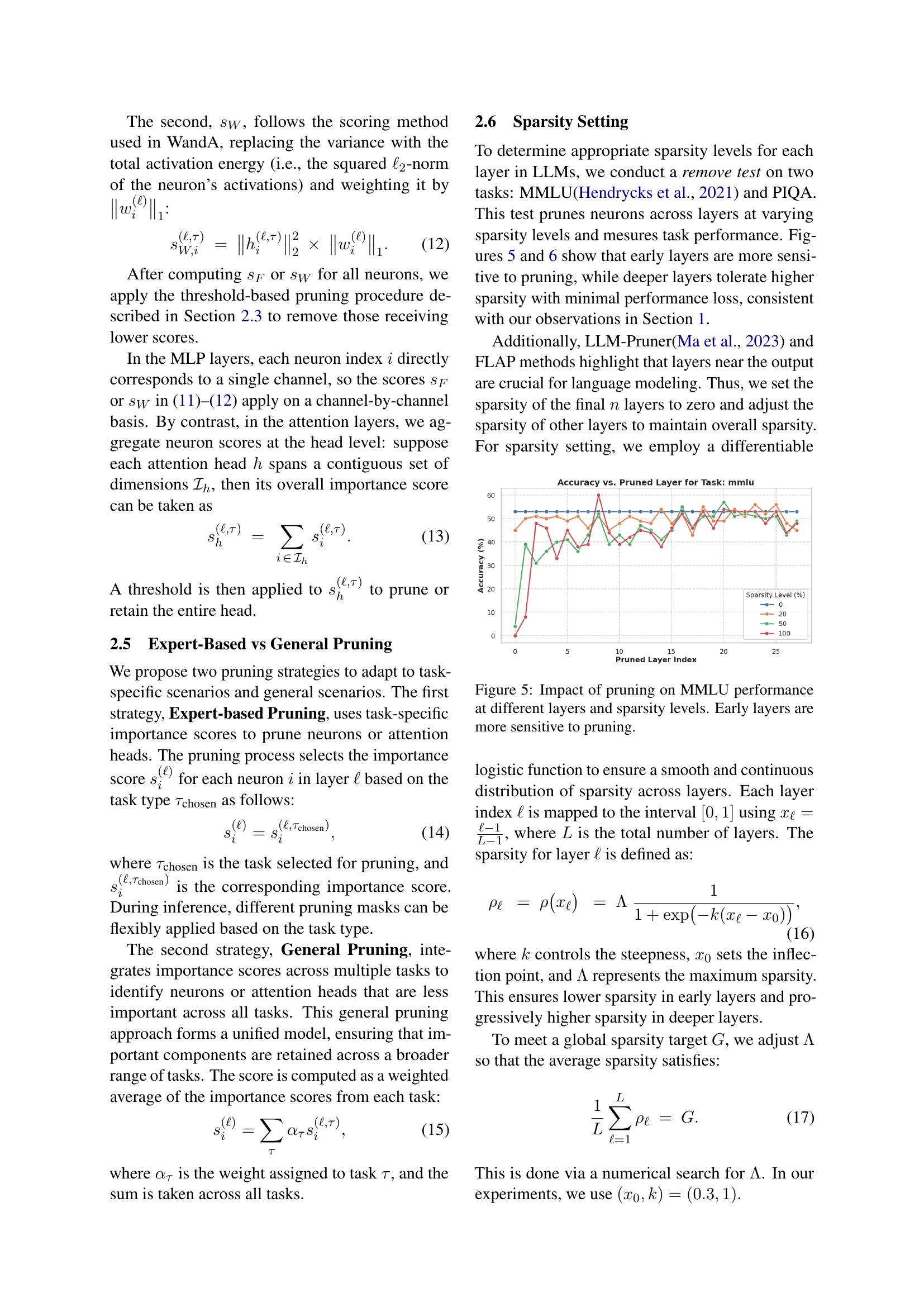
🔼 This figure shows how performance on the MMLU (Massive Multitask Language Understanding) benchmark changes when different layers of a large language model are pruned at varying sparsity levels (0%, 20%, 50%, 100%). The x-axis represents the layer index, indicating the depth of the layer within the model, with higher values corresponding to later layers. The y-axis displays the accuracy achieved on the MMLU task after pruning. Different lines represent different sparsity levels, illustrating the effect of removing increasing proportions of parameters. The results indicate that early layers (those with lower indices) are much more sensitive to pruning than later layers. A significant drop in accuracy is observed for early layers even at lower sparsity levels, whereas later layers exhibit greater resilience to pruning.
read the caption
Figure 5: Impact of pruning on MMLU performance at different layers and sparsity levels. Early layers are more sensitive to pruning.

🔼 This figure displays the results of an experiment that evaluated the impact of pruning on the PIQA task’s performance across different layers and sparsity levels within a large language model (LLM). The x-axis represents the index of the pruned layer, indicating the depth of the layer within the model. The y-axis represents the accuracy achieved on the PIQA task. Multiple lines are plotted, each representing a different sparsity level (percentage of the network pruned). The key observation is that deeper layers (higher layer indices) show greater robustness to pruning; they maintain higher accuracy even at increased sparsity levels compared to shallower layers. This suggests that the model’s crucial information for this specific task is concentrated in the deeper layers of the network.
read the caption
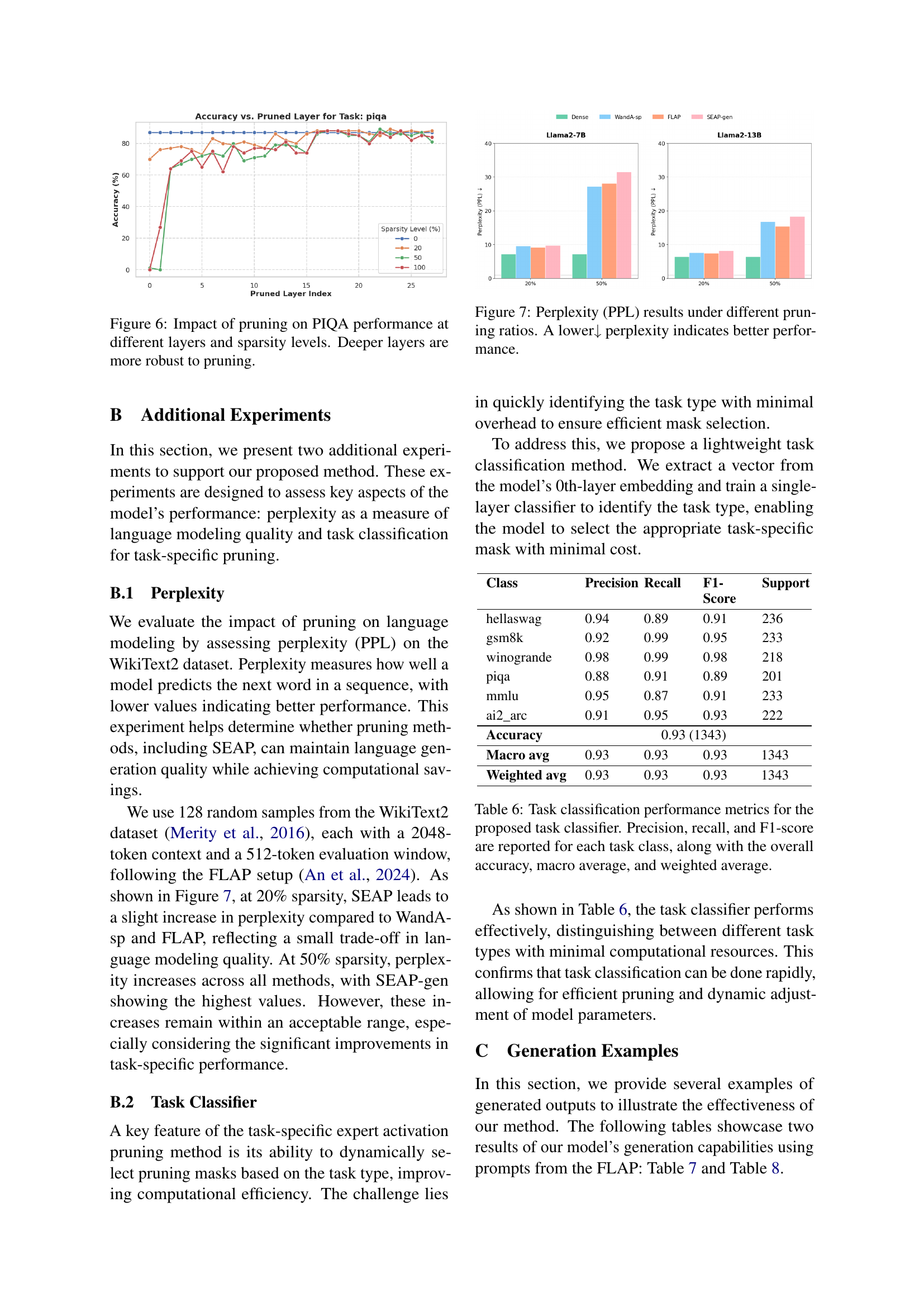
Figure 6: Impact of pruning on PIQA performance at different layers and sparsity levels. Deeper layers are more robust to pruning.

🔼 This figure displays the perplexity (PPL) scores achieved by different LLMs (Llama-2-7B and Llama-2-13B) under various pruning ratios (0%, 20%, and 50%). Perplexity is a metric that evaluates how well a language model predicts the next word in a sequence; lower perplexity indicates better performance. The graph visually demonstrates the trade-off between model compression (through pruning) and language modeling quality. It shows that as the pruning ratio increases, the perplexity generally increases, suggesting a slight degradation in the model’s ability to predict words accurately. However, the increase remains relatively small, particularly at lower pruning ratios, indicating that the proposed pruning methods maintain reasonably good language modeling capabilities even with significant model compression.
read the caption
Figure 7: Perplexity (PPL) results under different pruning ratios. A lower↓ perplexity indicates better performance.
More on tables
| Ratio | Method | Llama-2-7B | Llama-2-13B | ||
|---|---|---|---|---|---|
| Tokens/s | Up | Tokens/s | Up | ||
| 0% | Dense | 31.88 | 27.45 | ||
| 20% | WandA | 32.05 | ×1.01 | 28.01 | ×1.02 |
| FLAP | 38.90 | ×1.22 | 33.96 | ×1.24 | |
| SEAP-gen | 37.32 | ×1.17 | 33.02 | ×1.20 | |
| 50% | WandA | 31.24 | ×0.98 | 27.01 | ×0.98 |
| FLAP | 47.94 | ×1.50 | 43.45 | ×1.58 | |
| SEAP-gen | 47.10 | ×1.48 | 41.78 | ×1.52 | |
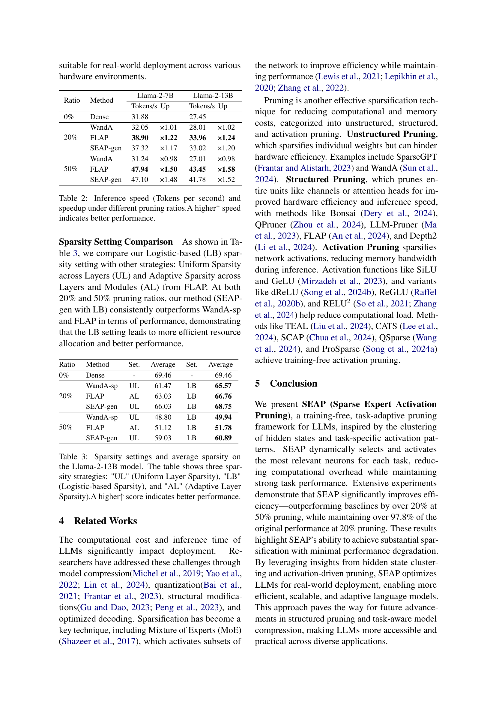
🔼 This table presents the inference speed, measured in tokens processed per second, for the Llama-2-7B and Llama-2-13B language models under various pruning ratios (0%, 20%, and 50%). It shows the speed improvement (speedup) achieved by pruning compared to the unpruned (dense) model. A higher number indicates better performance. The results are broken down for each model and pruning level, allowing for comparison of performance gains across different sparsity levels.
read the caption
Table 2: Inference speed (Tokens per second) and speedup under different pruning ratios.A higher↑ speed indicates better performance.
| Ratio | Method | Set. | Average | Set. | Average |
|---|---|---|---|---|---|
| 0% | Dense | - | 69.46 | - | 69.46 |
| 20% | WandA-sp | UL | 61.47 | LB | 65.57 |
| FLAP | AL | 63.03 | LB | 66.76 | |
| SEAP-gen | UL | 66.03 | LB | 68.75 | |
| 50% | WandA-sp | UL | 48.80 | LB | 49.94 |
| FLAP | AL | 51.12 | LB | 51.78 | |
| SEAP-gen | UL | 59.03 | LB | 60.89 |
🔼 This table compares three different sparsity strategies for pruning the Llama-2-13B language model: Uniform Layer Sparsity (UL), Logistic-based Sparsity (LB), and Adaptive Layer Sparsity (AL). The comparison is done at 20% and 50% pruning ratios. For each strategy and pruning ratio, the average performance across several downstream tasks is reported. A higher score indicates better performance, showing the effectiveness of each sparsity strategy in maintaining accuracy while reducing model size.
read the caption
Table 3: Sparsity settings and average sparsity on the Llama-2-13B model. The table shows three sparsity strategies: 'UL' (Uniform Layer Sparsity), 'LB' (Logistic-based Sparsity), and 'AL' (Adaptive Layer Sparsity).A higher↑ score indicates better performance.
| Pruning Ratio | Method | Llama-2-13B | |||||||
|---|---|---|---|---|---|---|---|---|---|
| WinoGrande | OBQA | HellaSwag | PIQA | ARC-c | ARC-e | BoolQ | Average | ||
| 0% | Dense | 72.14 | 45.20 | 79.37 | 80.52 | 48.98 | 79.42 | 80.58 | 69.46 |
| 20% | WandA-sp () | 67.40 | 42.80 | 74.52 | 78.40 | \ul48.64 | 76.73 | 70.49 | 65.57 |
| SEAP () | 71.98 | 43.60 | 78.73 | 80.69 | 48.46 | 77.61 | 74.68 | 67.96 | |
| SEAP-gen () | 69.85 | 43.20 | 78.13 | \ul80.47 | 48.55 | 78.58 | 72.54 | 67.33 | |
| FLAP () | 69.14 | 44.00 | 75.05 | 76.71 | 48.04 | 77.19 | \ul77.22 | 66.76 | |
| SEAP () | \ul70.64 | 44.80 | 79.12 | 80.69 | 47.95 | 76.85 | 76.82 | \ul68.12 | |
| SEAP-gen () | 70.09 | \ul44.20 | \ul78.97 | 80.09 | 50.17 | \ul78.37 | 79.36 | 68.75 | |
| 50% | WandA-sp () | 53.51 | 37.20 | 46.77 | 66.97 | 35.24 | 60.14 | 49.76 | 49.94 |
| SEAP () | 58.96 | 40.60 | 66.91 | 76.77 | \ul44.03 | \ul71.09 | \ul57.43 | 59.40 | |
| SEAP-gen () | \ul63.38 | 44.40 | 66.75 | 76.55 | 43.43 | \ul71.09 | 49.79 | 59.34 | |
| FLAP () | 55.17 | 38.20 | 53.82 | 67.41 | 33.11 | 58.42 | 56.36 | 51.78 | |
| SEAP () | 64.56 | 42.00 | 68.75 | \ul76.93 | 45.05 | 71.84 | 52.57 | \ul60.24 | |
| SEAP-gen () | 62.59 | \ul43.20 | \ul67.05 | 77.15 | 41.55 | 67.93 | 66.79 | 60.89 | |
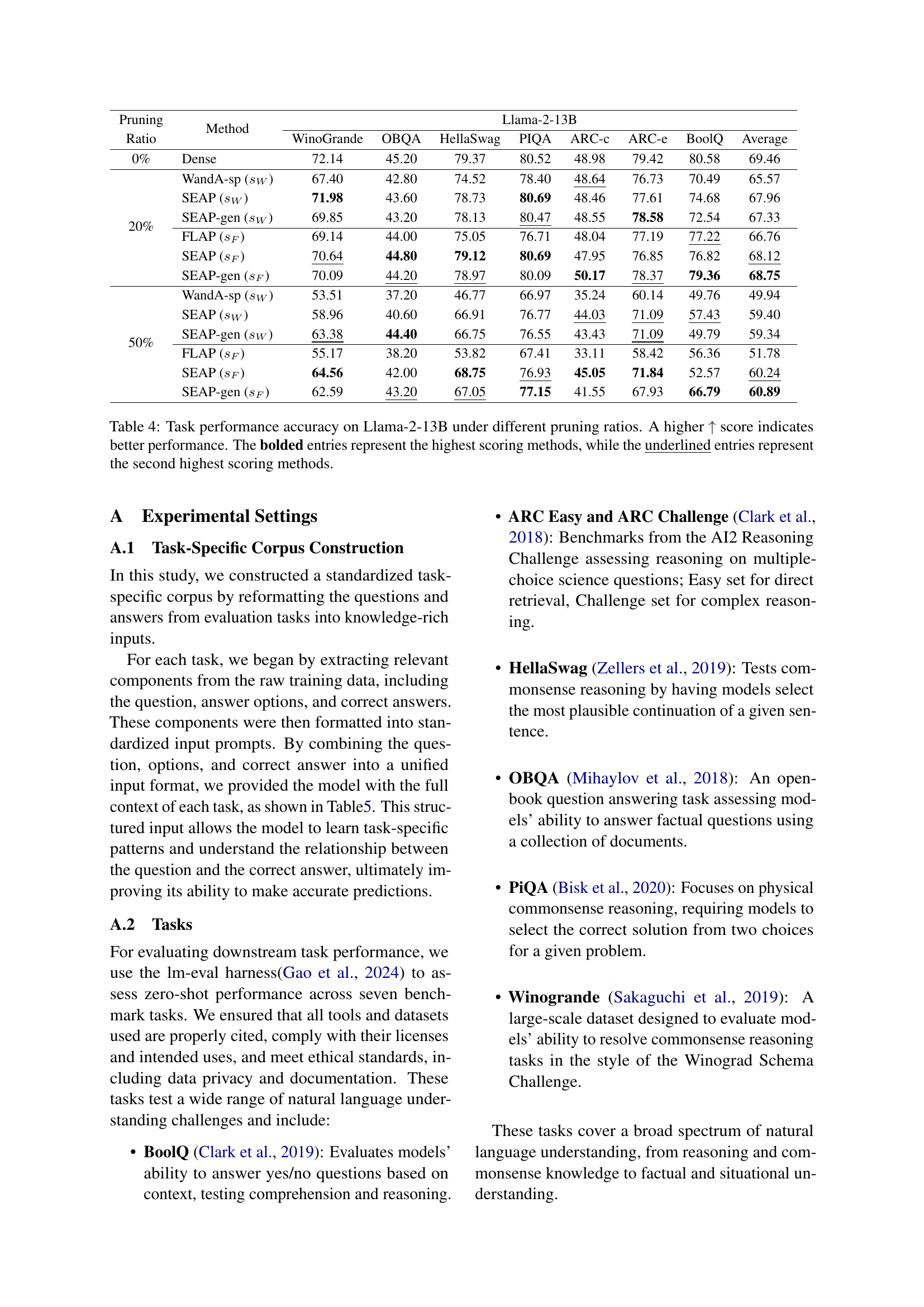
🔼 This table presents the results of the zero-shot task performance evaluation on the Llama-2-13B model using different pruning methods (SEAP, FLAP, and WandA) at various pruning ratios (0%, 20%, and 50%). The performance is measured across several downstream tasks: Winogrande, OBQA, HellaSwag, PIQA, ARC-C, ARC-e, and BoolQ. A higher score indicates better performance. The table highlights the best-performing method (bolded) and the second-best (underlined) for each task and pruning ratio, providing a comprehensive comparison of the different pruning techniques’ effectiveness on various tasks at different sparsity levels.
read the caption
Table 4: Task performance accuracy on Llama-2-13B under different pruning ratios. A higher ↑ score indicates better performance. The bolded entries represent the highest scoring methods, while the underlined entries represent the second highest scoring methods.
| Task | Example Prompt |
|---|---|
| HellaSwag | Then, the man writes over the snow covering the window of a car, and a woman wearing winter clothes smiles. Then, the man continues removing the snow on his car. |
| PIQA | How do I ready a guinea pig cage for its new occupants? Provide the guinea pig with a cage full of a few inches of bedding made of ripped paper strips, you will also need to supply it with a water bottle and a food dish. |
| OBQA | The sun is the source of energy for physical cycles on Earth: plants sprouting, blooming, and wilting. |
| WinoGrande | Katrina had the financial means to afford a new car while Monica did not, since Katrina had a high paying job. |
| ARC | One year, the oak trees in a park began producing more acorns than usual. The next year, the population of chipmunks in the park also increased. Which best explains why there were more chipmunks the next year? Food sources increased. |
| GSM8K | Natalia sold clips to 48 of her friends in April, and then she sold half as many clips in May. How many clips did Natalia sell altogether in April and May? Natalia sold 48/2 = 24 clips in May. Natalia sold 48 + 24 = 72 clips altogether in April and May. |
| BoolQ | All biomass goes through at least some of these steps: it needs to be grown, collected, dried, fermented, distilled, and burned… Does ethanol take more energy to make than it produces? False |
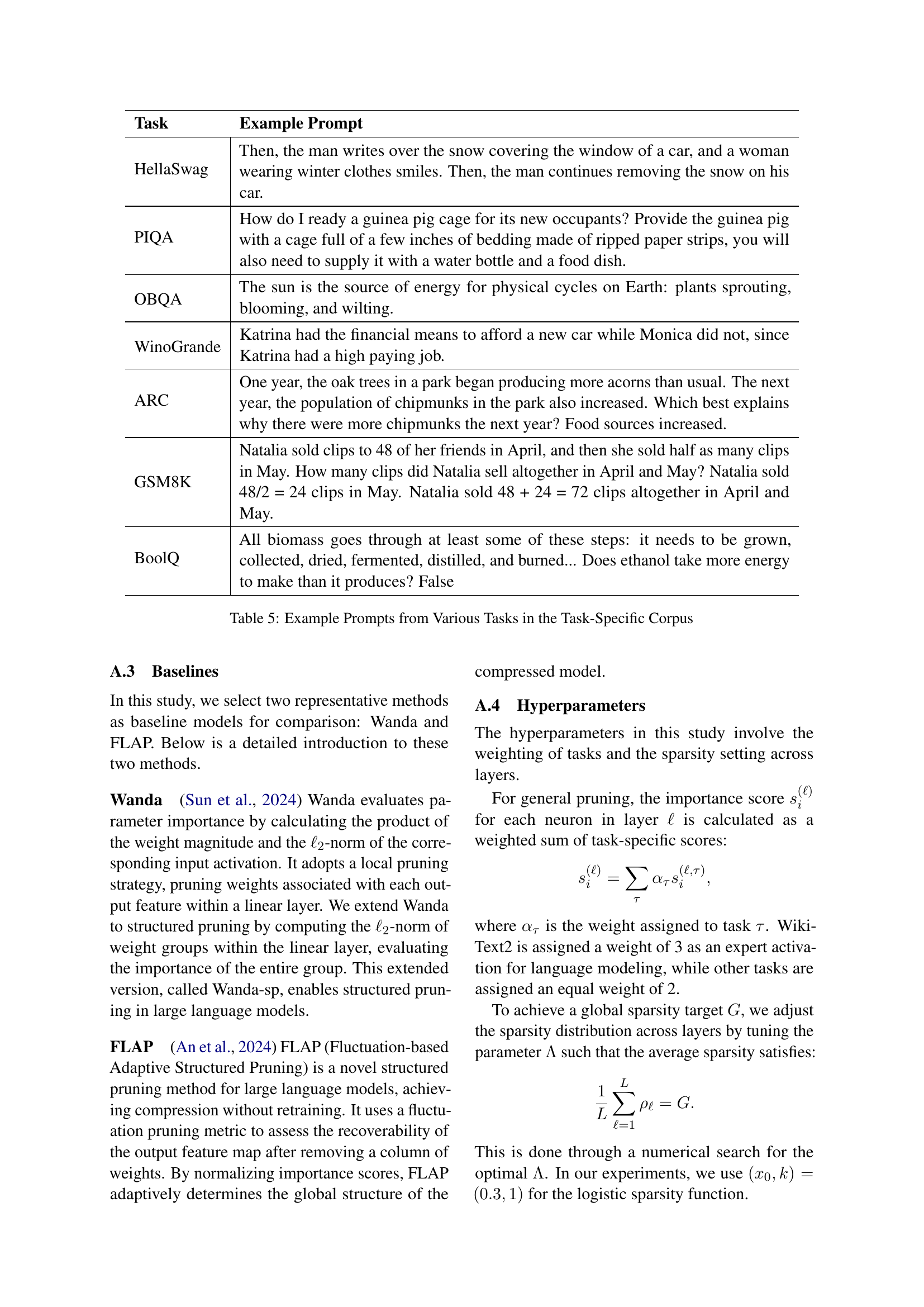
🔼 This table presents example prompts from seven different tasks used in the paper’s experiments. Each task represents a distinct category of natural language understanding challenges (e.g., commonsense reasoning, mathematical reasoning, scientific question answering). The prompts are constructed to be representative of the style and complexity found in the respective datasets. The purpose of including these examples is to illustrate the diversity of tasks and the nature of the inputs used to train and evaluate the model’s ability to extract task-specific activation patterns.
read the caption
Table 5: Example Prompts from Various Tasks in the Task-Specific Corpus
| Class | Precision | Recall | F1-Score | Support |
|---|---|---|---|---|
| hellaswag | 0.94 | 0.89 | 0.91 | 236 |
| gsm8k | 0.92 | 0.99 | 0.95 | 233 |
| winogrande | 0.98 | 0.99 | 0.98 | 218 |
| piqa | 0.88 | 0.91 | 0.89 | 201 |
| mmlu | 0.95 | 0.87 | 0.91 | 233 |
| ai2_arc | 0.91 | 0.95 | 0.93 | 222 |
| Accuracy | 0.93 (1343) | |||
| Macro avg | 0.93 | 0.93 | 0.93 | 1343 |
| Weighted avg | 0.93 | 0.93 | 0.93 | 1343 |
🔼 This table presents the performance of a task classifier designed to identify the type of downstream task. The classifier uses a single-layer model trained on embeddings from the 0th layer of the LLM. The results show precision, recall, F1-score, and support for each task category (HellaSwag, GSM8K, Winogrande, PiQA, MMLU, AI2-ARC). Overall accuracy, macro average, and weighted average are also provided, demonstrating the effectiveness and efficiency of the classifier in identifying task types for the subsequent application of task-specific pruning strategies.
read the caption
Table 6: Task classification performance metrics for the proposed task classifier. Precision, recall, and F1-score are reported for each task class, along with the overall accuracy, macro average, and weighted average.
| Model | Generated Sentences |
|---|---|
| LLaMA-7B 20% Pruned | AI can create a logo in seconds. But it’s not just a logo that you need to build a brand. A brand is a collection of ideas, emotions, and associations that people have about a product, service, or company. It’s the sum of all the things that make up a brand, and it’s what differentiates one brand from another. The most important thing to remember about branding is that it’s not just about the logo. |
| What is McDonald’s? McDonald’s is a fast-food restaurant franchise that serves burgers, fries, chicken nuggets, soft drinks, milkshakes, sundaes, salads, wraps, breakfast items (in some restaurants), desserts, and other items. The menu varies by country and region, but there are over 30,000 locations worldwide. | |
| LLaMA-7B 50% Pruned | AI can create a logo in seconds. The process of creating logotypes is called typestudy. A Log is a handwritten symbol or group of alphabets used in a script. In 1915, Eric Blake created the typeface Helvetica. It was a revival of handwriting from the Italian Renaissance. The first known example of handwriting is from a cave in Georgia, USA. It is dated 10,000 BCE. |
| What is McDonald’s? It is a small inn in an alley, a hundred yards or two from the gates. The tavern’s walls are thick, and it has a steeply pitched roof. Above the door there is carved a dragon’s flicked beak, with the words _Bow of Arrows_ carved in the sill. Inside, the tavern is large and well lit by daylight. There are three stairways leading to the north, all of which are occupied by men in armor. |
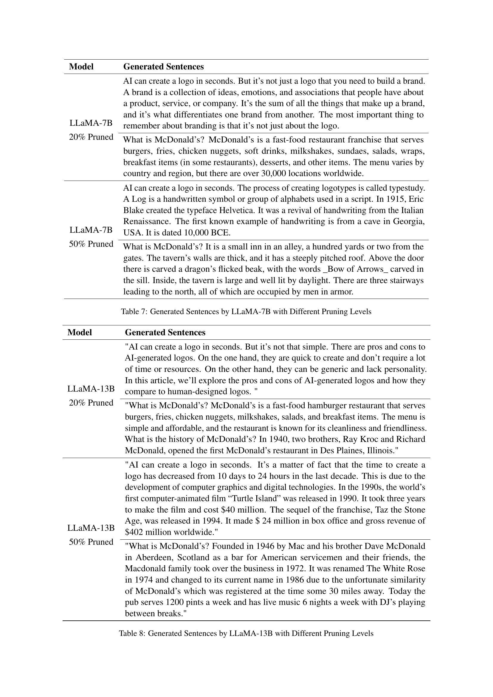
🔼 This table presents example sentences generated by the LLaMA-7B language model under different levels of pruning (0%, 20%, and 50%). It showcases the model’s ability to generate coherent text even with a significant reduction in parameters, illustrating the impact of SEAP on maintaining language generation capabilities while reducing model size.
read the caption
Table 7: Generated Sentences by LLaMA-7B with Different Pruning Levels
| Model | Generated Sentences |
|---|---|
| LLaMA-13B 20% Pruned | "AI can create a logo in seconds. But it’s not that simple. There are pros and cons to AI-generated logos. On the one hand, they are quick to create and don’t require a lot of time or resources. On the other hand, they can be generic and lack personality. In this article, we’ll explore the pros and cons of AI-generated logos and how they compare to human-designed logos. " |
| "What is McDonald’s? McDonald’s is a fast-food hamburger restaurant that serves burgers, fries, chicken nuggets, milkshakes, salads, and breakfast items. The menu is simple and affordable, and the restaurant is known for its cleanliness and friendliness. What is the history of McDonald’s? In 1940, two brothers, Ray Kroc and Richard McDonald, opened the first McDonald’s restaurant in Des Plaines, Illinois." | |
| LLaMA-13B 50% Pruned | "AI can create a logo in seconds. It’s a matter of fact that the time to create a logo has decreased from 10 days to 24 hours in the last decade. This is due to the development of computer graphics and digital technologies. In the 1990s, the world’s first computer-animated film “Turtle Island” was released in 1990. It took three years to make the film and cost $40 million. The sequel of the franchise, Taz the Stone Age, was released in 1994. It made $ 24 million in box office and gross revenue of $402 million worldwide." |
| "What is McDonald’s? Founded in 1946 by Mac and his brother Dave McDonald in Aberdeen, Scotland as a bar for American servicemen and their friends, the Macdonald family took over the business in 1972. It was renamed The White Rose in 1974 and changed to its current name in 1986 due to the unfortunate similarity of McDonald’s which was registered at the time some 30 miles away. Today the pub serves 1200 pints a week and has live music 6 nights a week with DJ’s playing between breaks." |
🔼 This table displays examples of text generated by the LLaMA-13B language model under different levels of pruning (20% and 50%). It showcases the model’s ability to generate coherent and relevant text even with a significant reduction in parameters. The examples illustrate the impact of pruning on the model’s output quality and demonstrate how different levels of sparsity may result in variations in the generated text. The differences highlight the trade-off between model efficiency and the quality of the generated text.
read the caption
Table 8: Generated Sentences by LLaMA-13B with Different Pruning Levels
Full paper#