TL;DR#
Diffusion models excel, but slow speed is a problem. Existing methods often trade quality or add complexity. This paper proposes RayFlow, a new diffusion framework. Unlike others, RayFlow guides each sample along a unique path to an instance-specific target, minimizing steps while preserving diversity and stability. The Time Sampler enhances training by focusing on key timesteps.
RayFlow generates high-quality images faster with better control and training efficiency than existing methods. It calculates a unified noise expectation, enabling compression without quality loss. By maximizing path probability, RayFlow minimizes instability. The results show that RayFlow consistently outperforms others, demonstrating its potential to be a leading solution in high-efficiency image generation.
Key Takeaways#
Why does it matter?#
This paper introduces RayFlow, a novel approach to diffusion modeling, offering improved image quality, speed, control, and training efficiency. It opens avenues for exploring and controlling diffusion processes, relevant to generative AI and beyond.
Visual Insights#

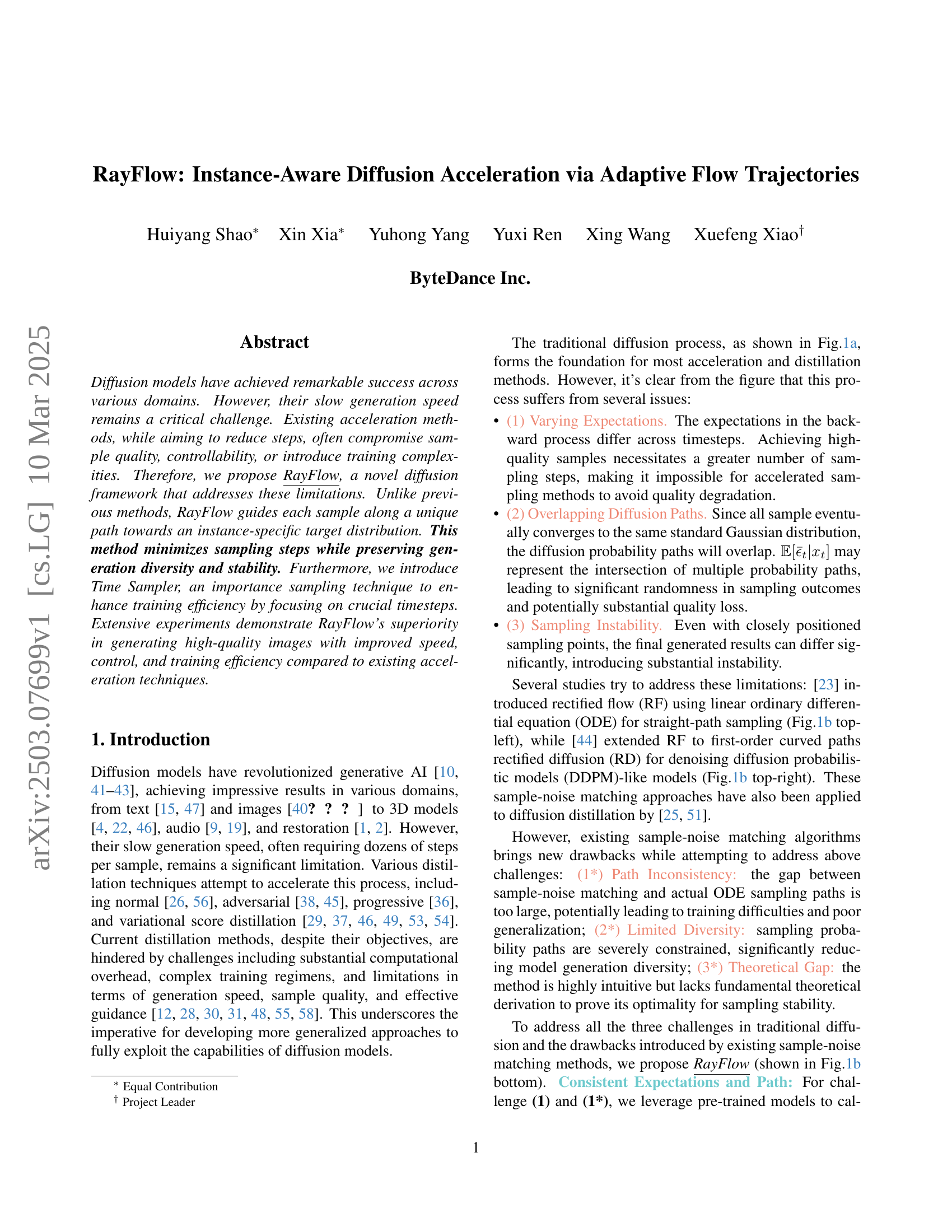
🔼 Figure 1(a) illustrates the conventional diffusion process. The forward diffusion process begins with a data sample and gradually adds Gaussian noise until it converges to a standard Gaussian distribution. The backward process reverses this, starting from the Gaussian distribution and iteratively removing noise to reconstruct a data sample. The figure visually demonstrates that the expectations for the backward process (denoising) change over timesteps, and that the paths of different samples can overlap which can lead to quality degradation.
read the caption
(a) The forward and backward process of traditional diffusion.
| COCO-5k | ImageNet | Cifar-100 | Cifar-10 | |||||||||
| Module | Clip | Aes | FID | Clip | Aes | FID | Clip | Aes | FID | Clip | Aes | FID |
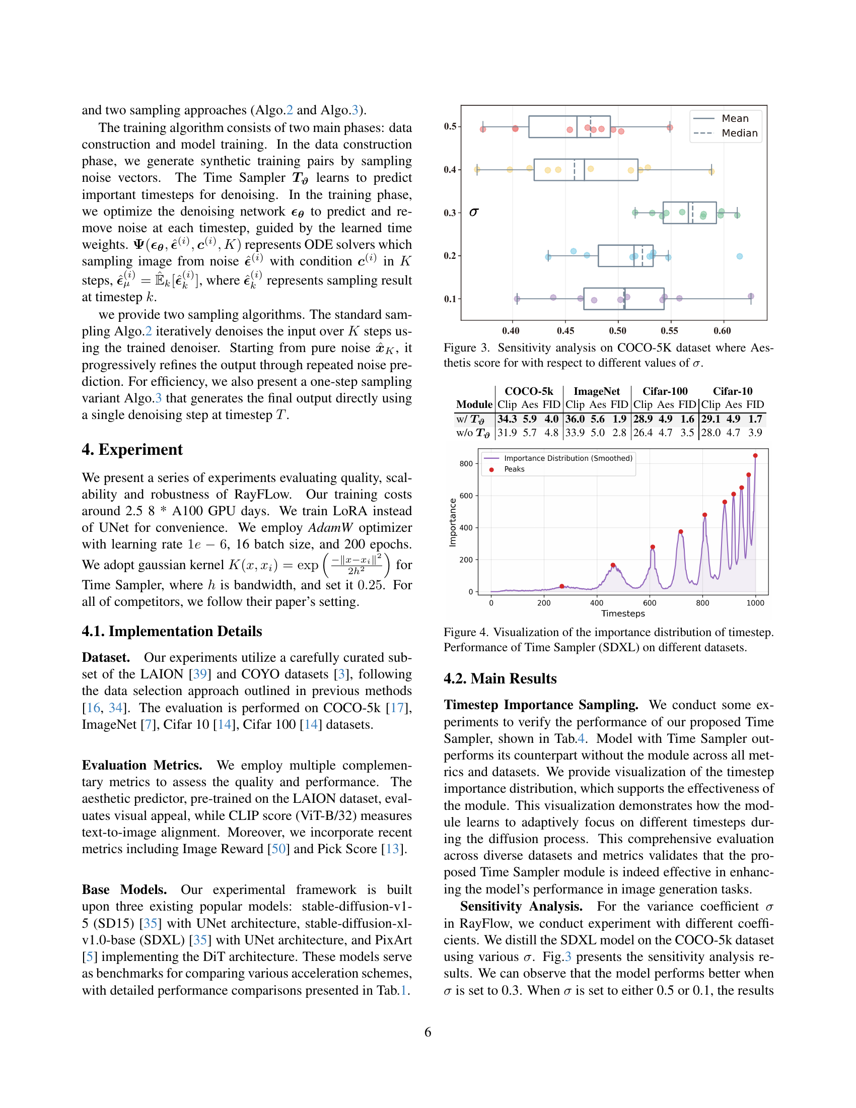
| w/ | 34.3 | 5.9 | 4.0 | 36.0 | 5.6 | 1.9 | 28.9 | 4.9 | 1.6 | 29.1 | 4.9 | 1.7 |
| w/o | 31.9 | 5.7 | 4.8 | 33.9 | 5.0 | 2.8 | 26.4 | 4.7 | 3.5 | 28.0 | 4.7 | 3.9 |
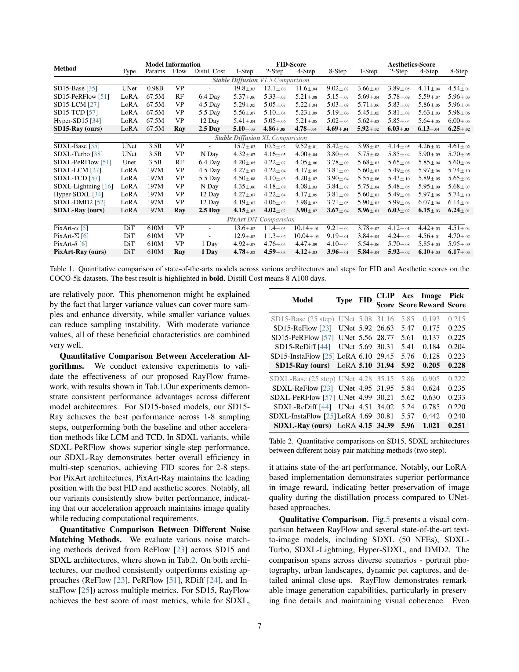
🔼 This table presents a quantitative comparison of several state-of-the-art image generation models. It shows how different models (including various versions of Stable Diffusion and PixArt) perform across different numbers of sampling steps (1-step to 8-step), using different architectures (UNet and DiT), and employing various diffusion acceleration methods (VP, RF, Ray). The models are evaluated on the COCO-5k dataset using FID (Fréchet Inception Distance) and Aesthetics scores. The best-performing model for each metric and number of steps is highlighted in bold. The ‘Distill Cost’ column indicates the approximate training time using 8 A100 GPUs. This table helps illustrate the performance trade-offs between speed, model complexity and image quality for various models and acceleration techniques.
read the caption
Table 1: Quantitative comparison of state-of-the-arts models across various architectures and steps for FID and Aesthetic scores on the COCO-5k datasets. The best result is highlighted in bold. Distill Cost means 8 A100 days.
In-depth insights#
Adaptive RayFlow#
While “Adaptive RayFlow” isn’t explicitly mentioned, one can infer its essence from the paper’s core contributions. The core is adapting the diffusion process to each instance, guiding each sample along a unique path towards its specific target. The paper minimizes sampling steps while preserving generation diversity and stability. The use of the Time Sampler, an importance sampling technique, further exemplifies the adaptive nature by focusing on crucial timesteps during training, thus improving training efficiency. By leveraging pre-trained models to calculate a unified noise expectation the proposed method achieves efficient step compression without quality degradation. Overall, this adaptive approach seems key to overcoming the limitations of traditional diffusion methods, offering a more efficient and controllable generative process.
Varying Expectation#
Varying Expectations in generative models, especially diffusion models, refer to the challenge that the ideal or anticipated outcome of the reverse diffusion process differs significantly across timesteps. Early timesteps might require broad adjustments to the noise distribution, while later timesteps demand precise refinement to generate realistic details. This variance necessitates a large number of sampling steps to ensure high-quality output, as a single sampling strategy becomes insufficient. Acceleration methods often struggle to maintain quality because they reduce steps, inevitably overlooking subtle but crucial adjustments at certain timesteps. Addressing this requires adaptive sampling strategies or models capable of handling diverse refinement scales efficiently, balancing global structure and fine-grained detail.
Overlapping Paths#
Overlapping paths in the context of diffusion models can significantly hinder the generation process. If the probability paths of different samples overlap considerably during the reverse diffusion, it leads to a loss of diversity and potential quality degradation. This is because the model struggles to distinguish between the unique characteristics of each sample, causing them to converge towards similar outputs. The randomness in the sampling process exacerbates this issue, as slight variations in the initial noise can result in drastically different final results due to the overlapping paths. Mitigating this requires strategies that ensure distinct trajectories for each sample, preventing them from getting ’lost’ in the shared probability space and preserving individual sample identity.
Sampling Instable#
Sampling instability in diffusion models arises from the sensitivity of the generative process to minor variations in sampling points, leading to substantial differences in the final output. This is caused by overlapping diffusion paths, where convergence to a common Gaussian distribution introduces randomness and quality loss. Even closely positioned sampling steps can yield significantly different results, posing challenges for consistent and reliable generation. Mitigating this instability is critical for improving the overall quality and stability of diffusion models, requiring methods that reduce sensitivity to sampling variations and promote more deterministic behavior.
Time Sampler#
Time Sampler enhances training efficiency by focusing on crucial timesteps, moving beyond uniform sampling. It identifies the most informative points, thereby reducing redundancy and computational cost. Integrating Stochastic Stein Discrepancies (SSD) with neural networks, it approximates the optimal sampling distribution. This dynamic adjustment minimizes variance in the training loss estimator, which is critical for faster convergence and better model performance. By prioritizing key timesteps, Time Sampler facilitates more efficient learning, making the diffusion model more practical.
More visual insights#
More on figures

🔼 This figure illustrates RayFlow’s forward and reverse processes. Unlike traditional diffusion models that converge to a single Gaussian distribution, RayFlow guides each sample along a unique trajectory towards an instance-specific target distribution. The forward process adds noise, while the reverse process denoises. The illustration depicts how each sample is guided along its own trajectory, enabling the generation of high-quality images with minimal sampling steps while preserving generation diversity and stability.
read the caption
(b) The forward and backward process of our diffusion method.

🔼 Figure 1 compares the forward and backward diffusion processes in traditional diffusion models with those in RayFlow. The traditional method shows limitations: varying expectations across timesteps (leading to quality loss in accelerated sampling), overlapping diffusion paths (reducing sampling diversity and causing instability), and overall sampling instability. RayFlow aims to address these through consistent expectations via pre-trained models, guiding each sample on an individual path to reduce overlaps and improve diversity, and achieving theoretical guarantees for improved sampling stability.
read the caption
Figure 1: The comparision of different diffusion process.

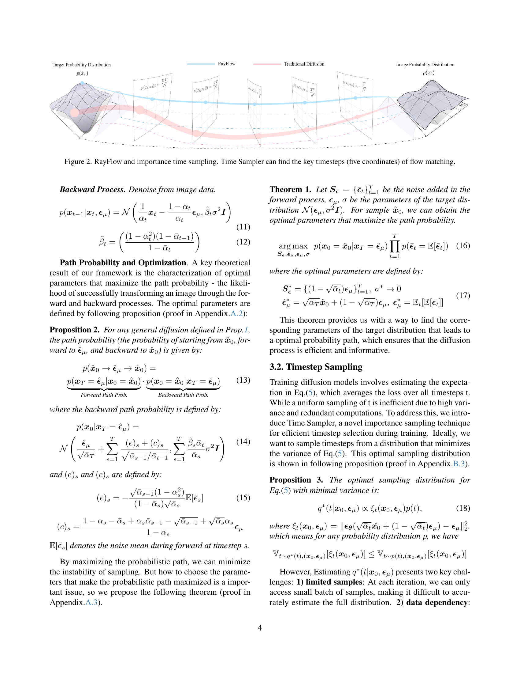
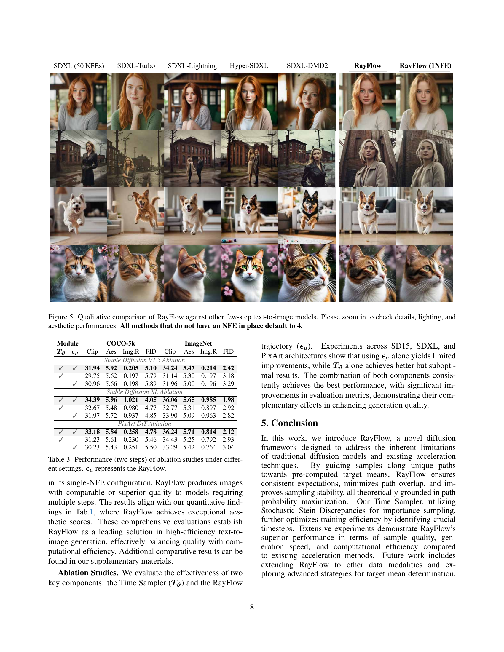
🔼 This figure illustrates the core concepts of RayFlow and its Time Sampler component. The left panel depicts the traditional diffusion process, showing how samples traverse a wide range of timesteps before reaching the target distribution. The paths are highly varied and may overlap substantially, leading to issues with stability and sampling quality. In contrast, the right panel shows the RayFlow process. Each sample follows a unique path directly toward its instance-specific target distribution. Note that each trajectory smoothly converges towards its mean instead of transitioning through the typical Gaussian distribution. This drastically reduces sampling steps. The Time Sampler component is highlighted showing how it identifies key timesteps for training, reducing computational overhead. These key timesteps (five in this example) are visualized as the coordinates on the simplified diffusion path.
read the caption
Figure 2: RayFlow and importance time sampling. Time Sampler can find the key timesteps (five coordinates) of flow matching.

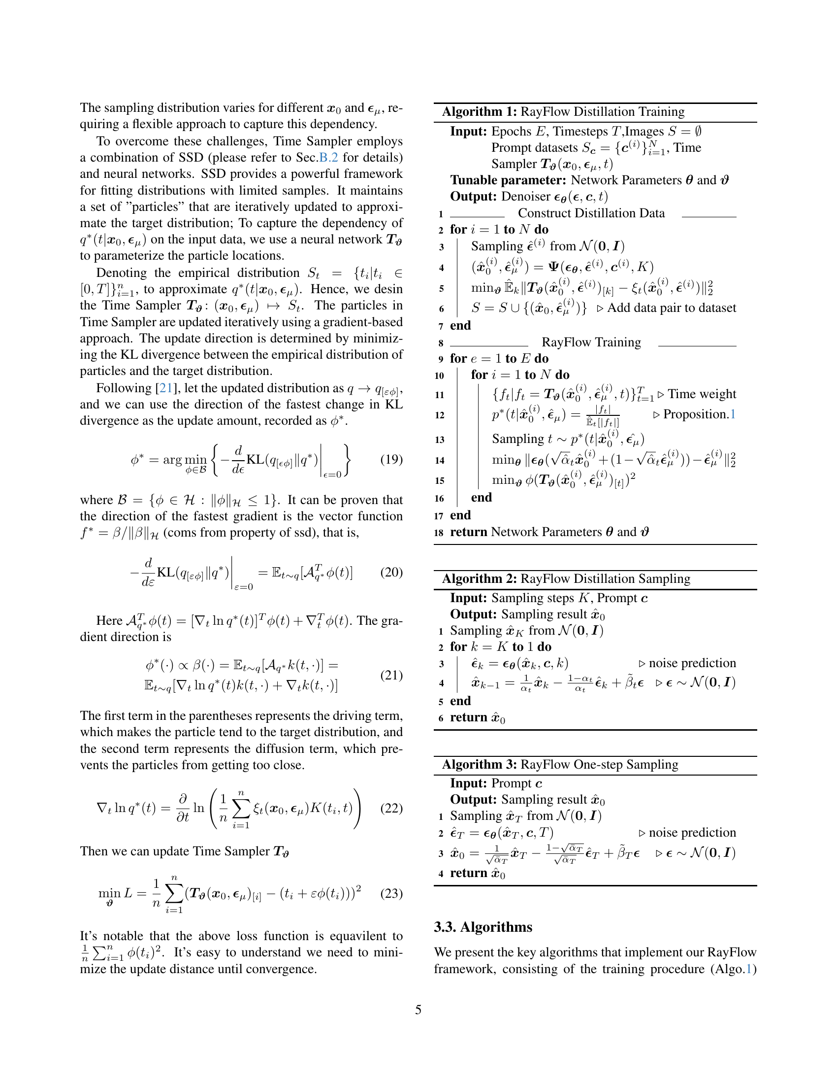
🔼 This figure displays the results of a sensitivity analysis performed on the COCO-5K dataset to determine the impact of the variance coefficient (σ) on the model’s performance. The analysis assesses the relationship between different values of σ and the resulting aesthetic scores achieved by the model. The box plot visualization effectively shows the distribution of aesthetic scores for various σ values, highlighting how changes in this parameter affect the model’s output quality.
read the caption
Figure 3: Sensitivity analysis on COCO-5K dataset where Aesthetis score for with respect to different values of σ𝜎\sigmaitalic_σ.
More on tables
| Method | Model Information | FID-Score | Aesthetics-Score | |||||||||
| Type | Params | Flow | Distill Cost | 1-Step | 2-Step | 4-Step | 8-Step | 1-Step | 2-Step | 4-Step | 8-Step | |
| Stable Diffusion V1.5 Comparision | ||||||||||||
| SD15-Base [35] | UNet | 0.98B | VP | - | 19.8.03 | 12.1.06 | 11.6.04 | 9.02.02 | 3.66.03 | 3.89.05 | 4.11.04 | 4.54.01 |
| SD15-PeRFlow [51] | LoRA | 67.5M | RF | 6.4 Day | 5.37.06 | 5.33.03 | 5.21.08 | 5.15.07 | 5.69.04 | 5.78.09 | 5.59.07 | 5.96.03 |
| SD15-LCM [27] | LoRA | 67.5M | VP | 4.5 Day | 5.29.05 | 5.05.07 | 5.22.04 | 5.03.09 | 5.71.06 | 5.83.07 | 5.86.05 | 5.96.04 |
| SD15-TCD [57] | LoRA | 67.5M | VP | 5.5 Day | 5.56.07 | 5.10.04 | 5.23.09 | 5.19.06 | 5.45.05 | 5.81.08 | 5.63.03 | 5.98.06 |
| Hyper-SD15 [34] | LoRA | 67.5M | VP | 12 Day | 5.41.04 | 5.05.06 | 5.21.05 | 5.02.04 | 5.62.03 | 5.85.04 | 5.64.05 | 6.00.05 |
| SD15-Ray (ours) | LoRA | 67.5M | Ray | 2.5 Day | 5.10.03 | 4.86.05 | 4.78.04 | 4.69.04 | 5.92.02 | 6.03.03 | 6.13.04 | 6.25.02 |
| Stable Diffusion XL Comparision | ||||||||||||
| SDXL-Base [35] | UNet | 3.5B | VP | - | 15.7.03 | 10.5.02 | 9.52.01 | 8.42.04 | 3.98.02 | 4.14.05 | 4.26.03 | 4.61.02 |
| SDXL-Turbo [38] | UNet | 3.5B | VP | N Day | 4.32.07 | 4.16.05 | 4.00.04 | 3.80.06 | 5.75.08 | 5.85.04 | 5.90.09 | 5.70.05 |
| SDXL-PeRFlow [51] | Unet | 3.5B | RF | 6.4 Day | 4.20.05 | 4.22.07 | 4.05.06 | 3.78.09 | 5.68.03 | 5.65.08 | 5.85.04 | 5.60.06 |
| SDXL-LCM [27] | LoRA | 197M | VP | 4.5 Day | 4.27.07 | 4.22.04 | 4.17.05 | 3.81.09 | 5.60.03 | 5.49.08 | 5.97.06 | 5.74.10 |
| SDXL-TCD [57] | LoRA | 197M | VP | 5.5 Day | 4.50.08 | 4.10.03 | 4.20.07 | 3.90.04 | 5.55.06 | 5.43.10 | 5.89.05 | 5.65.03 |
| SDXL-Lightning [16] | LoRA | 197M | VP | N Day | 4.35.06 | 4.18.09 | 4.08.03 | 3.84.07 | 5.75.04 | 5.48.05 | 5.95.09 | 5.68.07 |
| Hyper-SDXL [34] | LoRA | 197M | VP | 12 Day | 4.27.07 | 4.22.04 | 4.17.05 | 3.81.09 | 5.60.03 | 5.49.08 | 5.97.06 | 5.74.10 |
| SDXL-DMD2 [52] | LoRA | 197M | VP | 12 Day | 4.19.02 | 4.06.03 | 3.98.02 | 3.71.05 | 5.90.03 | 5.99.06 | 6.07.04 | 6.14.01 |
| SDXL-Ray (ours) | LoRA | 197M | Ray | 2.5 Day | 4.15.03 | 4.02.02 | 3.90.02 | 3.67.04 | 5.96.01 | 6.03.02 | 6.15.03 | 6.24.01 |
| PixArt DiT Comparision | ||||||||||||
| PixArt- [5] | DiT | 610M | VP | - | 13.6.02 | 11.4.03 | 10.14.01 | 9.21.04 | 3.78.02 | 4.12.01 | 4.42.03 | 4.51.04 |
| PixArt- [6] | DiT | 610M | VP | - | 12.9.02 | 11.3.02 | 10.04.03 | 9.19.01 | 3.84.04 | 4.24.02 | 4.56.01 | 4.70.02 |
| PixArt- [6] | DiT | 610M | VP | 1 Day | 4.92.07 | 4.76.05 | 4.47.09 | 4.10.04 | 5.54.06 | 5.70.08 | 5.85.03 | 5.95.09 |
| PixArt-Ray (ours) | DiT | 610M | Ray | 1 Day | 4.78.02 | 4.59.03 | 4.12.03 | 3.96.01 | 5.84.04 | 5.92.02 | 6.10.03 | 6.17.03 |
🔼 This table presents a quantitative comparison of different noise matching methods used in diffusion models, specifically focusing on the SD15 and SDXL architectures. The comparison uses two sampling steps and evaluates various metrics including FID (Fréchet Inception Distance), CLIP (Contrastive Language–Image Pre-training) score, and others to assess the quality of generated images. It shows how these different methods compare in terms of image quality and efficiency.
read the caption
Table 2: Quantitative comparisons on SD15, SDXL architectures between different noisy pair matching methods (two step).
| Model | Type | FID | CLIP Score | Aes Score | Image Reward | Pick Score |
| SD15-Base (25 step) | UNet | 5.08 | 31.16 | 5.85 | 0.193 | 0.215 |
| SD15-ReFlow [23] | UNet | 5.92 | 26.63 | 5.47 | 0.175 | 0.225 |
| SD15-PeRFlow [57] | UNet | 5.56 | 28.77 | 5.61 | 0.137 | 0.225 |
| SD15-ReDiff [44] | UNet | 5.69 | 30.31 | 5.41 | 0.184 | 0.204 |
| SD15-InstaFlow [25] | LoRA | 6.10 | 29.45 | 5.76 | 0.128 | 0.223 |
| SD15-Ray (ours) | LoRA | 5.10 | 31.94 | 5.92 | 0.205 | 0.228 |
| SDXL-Base (25 step) | UNet | 4.28 | 35.15 | 5.86 | 0.905 | 0.222 |
| SDXL-ReFlow [23] | UNet | 4.95 | 31.95 | 5.84 | 0.624 | 0.235 |
| SDXL-PeRFlow [57] | UNet | 4.99 | 30.21 | 5.62 | 0.630 | 0.233 |
| SDXL-ReDiff [44] | UNet | 4.51 | 34.02 | 5.24 | 0.785 | 0.220 |
| SDXL-InstaFlow [25] | LoRA | 4.69 | 30.81 | 5.57 | 0.442 | 0.240 |
| SDXL-Ray (ours) | LoRA | 4.15 | 34.39 | 5.96 | 1.021 | 0.251 |
🔼 This table presents the results of ablation studies conducted to evaluate the impact of individual components of the RayFlow model on its performance. The experiments were run using two sampling steps. The table compares the model’s performance with different combinations of the Time Sampler (To) and the RayFlow trajectory (ϵμ). The results are shown across multiple evaluation metrics, including FID, CLIP, image reward, and aesthetic scores, on three different datasets: COCO-5k, ImageNet, and PixArt-DiT.
read the caption
Table 3: Performance (two steps) of ablation studies under different settings. ϵμsubscriptbold-italic-ϵ𝜇\bm{\epsilon}_{\mu}bold_italic_ϵ start_POSTSUBSCRIPT italic_μ end_POSTSUBSCRIPT represents the RayFlow.
Full paper#