Florenz: Scaling Laws for Systematic Generalization in Vision-Language Models

2503.09443

Julian Spravil et el.

🤗 2025-03-19

TL;DR
#

Current vision-language models struggle with multilinguality, sacrificing downstream performance and facing lexical ambiguities. This paper addresses these issues by studying systematic generalization with monolingual VLMs for multilingual tasks. It focuses on the impact of model size and training data, aiming to improve cross-lingual transfer without extensive multilingual pre-training.

The paper introduces a new model family, Florenz, based on Florence-2 and Gemma-2, and trained it on a synthetic dataset with incomplete language coverage. It shows that indirectly learning task-language pairs adheres to a scaling law. The paper demonstrates that image captioning abilities can emerge in a specific language even with translation data only and achieves competitive results on downstream tasks.

Key Takeaways
#

Why does it matter?
#

This work matters because it studies how well monolingual models generalize to multilingual tasks. It addresses the crucial issue of accessibility in vision-language models, providing insights on creating models that perform well in multiple languages without needing extensive data for each. It also introduces a method for dataset creation that opens new avenues for future research.

Visual Insights
#

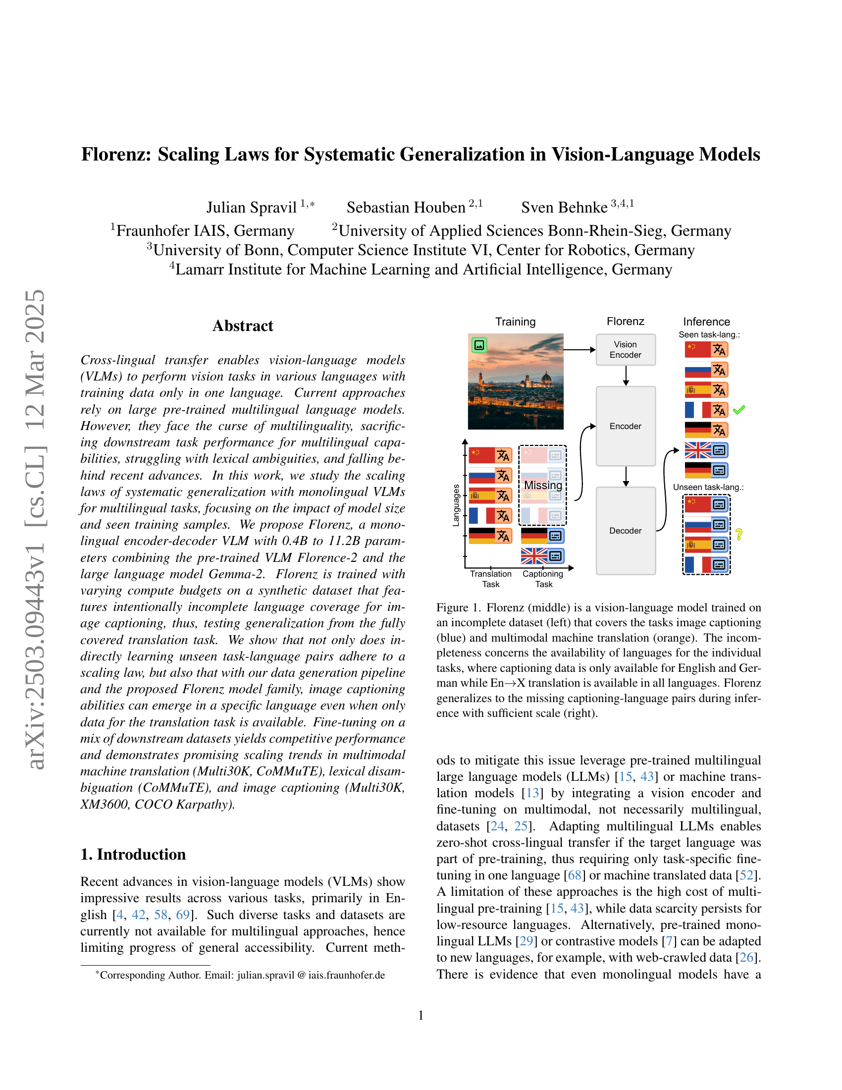
🔼 Figure 1 illustrates the architecture and training process of the Florenz vision-language model. The diagram shows three parts: (left) an incomplete training dataset, (middle) the Florenz model architecture, and (right) the model’s inference process. The training dataset includes image captioning tasks (in blue) and multimodal machine translation tasks (in orange). Critically, the training data for image captioning is only available in English and German, while the machine translation data covers multiple languages (English to other languages). The Florenz model, designed as a monolingual encoder-decoder VLM, leverages pre-trained monolingual models. The diagram demonstrates that despite limited training data for image captioning, the Florenz model generalizes to other languages (unseen languages) at inference time. The model’s ability to do this is linked to a scaling law, which means that a larger model with increased parameter count and training data results in better cross-lingual generalization.
read the caption
Figure 1: Florenz (middle) is a vision-language model trained on an incomplete dataset (left) that covers the tasks image captioning (blue) and multimodal machine translation (orange). The incompleteness concerns the availability of languages for the individual tasks, where captioning data is only available for English and German while En→→\rightarrow→X translation is available in all languages. Florenz generalizes to the missing captioning-language pairs during inference with sufficient scale (right).

	Context Length
Model	0	32	64	128	256
NLLB-600M [13]	50.0	55.3	54.7	55.3	54.0
NLLB-3.3B [13]	50.0	60.7	64.0	63.3	63.3

🔼 This table presents the results of a binary disambiguation task on the CoMMuTE English-to-German dataset. The experiment uses the NLLB machine translation model with varying context lengths (0, 32, 64, 128, 256) added to the input captions. The goal is to determine how the model’s accuracy in disambiguating lexically ambiguous words changes based on the length of the added context. Two different sizes of NLLB models were used, demonstrating that both the context length and the model size significantly influence the performance.
read the caption
Table 1: Accuracy (%) of binary disambiguation on the CoMMuTE En→→\rightarrow→De subset [24] using the context-enhanced machine translation model NLLB [13] for various context lengths. Note that longer context and larger model result in better accuracy.

In-depth insights
#

Monolingual Scaling
#

Monolingual scaling in vision-language models (VLMs) offers a fascinating avenue for cross-lingual transfer. The conventional wisdom favors multilingual pre-training, but focusing on scaling monolingual models presents a compelling alternative. It allows for concentrated resource allocation, potentially leading to superior performance in the source language and surprising cross-lingual generalization. The Florenz paper investigates this, proposing a monolingual encoder-decoder VLM that, through strategic data generation and scaling, achieves impressive results in multilingual tasks. By training primarily on English and German data, the model demonstrates the ability to caption images in languages it has only encountered in translation tasks, suggesting that the capacity gained through scaling enables it to extrapolate task knowledge.

Florenz’s Design
#

Florenz leverages a standard transformer encoder-decoder architecture, combining the strengths of Florence-2 for visual encoding and Gemma-2 for language decoding. This allows the model to process visual information and generate coherent textual descriptions. The model’s design focuses on efficient transfer learning and systematic generalization. Model sizes range from 0.4B to 11.2B parameters, allowing for scalability. The image embeddings and a task prompt are fed into the encoder and then passed to the decoder. The decoder consists of Sentencepiece tokenizer trained for Gemini.

Synthetic Data
#

While the provided paper doesn’t explicitly discuss “Synthetic Data” under that specific heading, the study’s core methodology revolves around its implicit use. The authors generate a synthetic dataset with intentionally incomplete language coverage to train their Florenz model. This is a clever approach to test systematic generalization. By training on data where certain language-task pairings are missing (e.g., captioning in specific languages), they force the model to learn underlying relationships between language and vision, rather than simply memorizing training examples. The performance of Florenz on unseen task-language pairs then becomes a measure of its ability to generalize from the available data. This approach cleverly circumvents the limitations of relying solely on pre-existing, comprehensive datasets, which are often unavailable in multilingual contexts. The model’s ability to caption images in a language even when only translation data is available indicates that the synthetic data generation successfully imparts cross-lingual understanding.

Prefix Generalize
#

Decoder prefixes act as crucial keys to unlock generalization in vision-language models (VLMs). While cross-entropy loss decreases, models often struggle to generate text in the desired language, defaulting to training languages like German or English. Adding a simple prefix in the target language seeds the output, enabling caption generation without explicit exposure to target language captioning data. This suggests that systematic generalization relies on the model’s ability to recognize and utilize language cues, prompting the generation process in the correct language context. This points to a simple but effective mechanism for activating dormant multilingual capabilities. The pre-training scaling laws suggest that the number of seen samples has a secondary role for systematic generalization.

Task Balance
#

Balancing tasks is crucial in multilingual learning to prevent the model from overfitting to dominant languages or tasks. An effective balance ensures fair representation and learning across all languages and tasks, enhancing generalization. Techniques involve adjusting sampling probabilities to ensure equal representation from each task-language combination. Careful attention to task balance leads to models that are robust and perform consistently across diverse linguistic scenarios.

More visual insights
#

More on figures

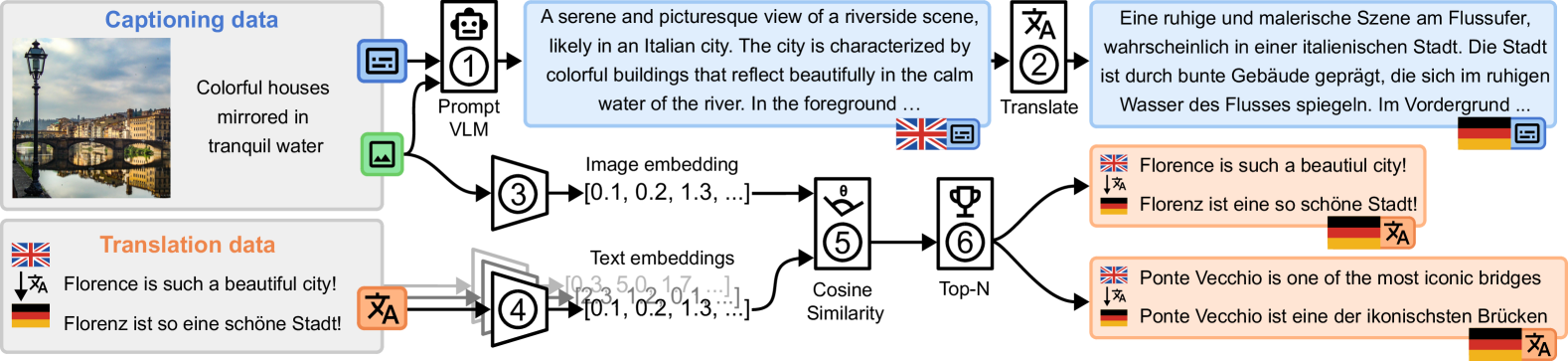
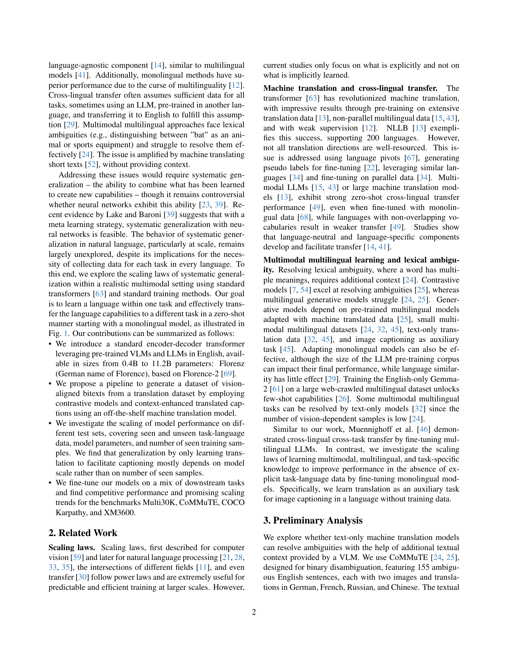
🔼 This figure illustrates the process of creating a multilingual multimodal dataset. The input consists of an image dataset with short captions or alt text, and a parallel translation dataset (bitexts) in English and German. The pipeline involves these steps: 1. Detailed Description Generation: An image and its short caption are fed into a Vision-Language Model (VLM) to generate a more detailed description in English. 2. Translation: The detailed English description is then translated into the target language (German). 3. Embedding: Both the image (using image embeddings) and all English sentences from the parallel translation dataset (using text embeddings) are converted into vector representations in a shared vector space. 4. Cosine Similarity Calculation: Cosine similarity is computed to measure the similarity between the image embedding and each English sentence embedding. 5. Top-N Matching: The top N most similar image-translation pairs are selected, creating a new dataset with matched image and translated descriptions.
read the caption
Figure 2: Dataset generation pipeline. Input is an image dataset with short captions or alt texts and a translation dataset with bitexts in English and the target language German. (1) Image and short caption are fed into a VLM to generate a detailed English description, which is (2) translated into the target language. (3) The image and (4) all English sentences of the translation dataset are embedded in a shared vector space. (5) Cosine similarity is calculated and (6) top-N matching pairs the most similar images and translations.

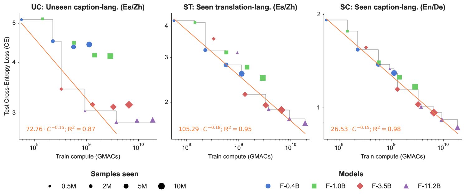
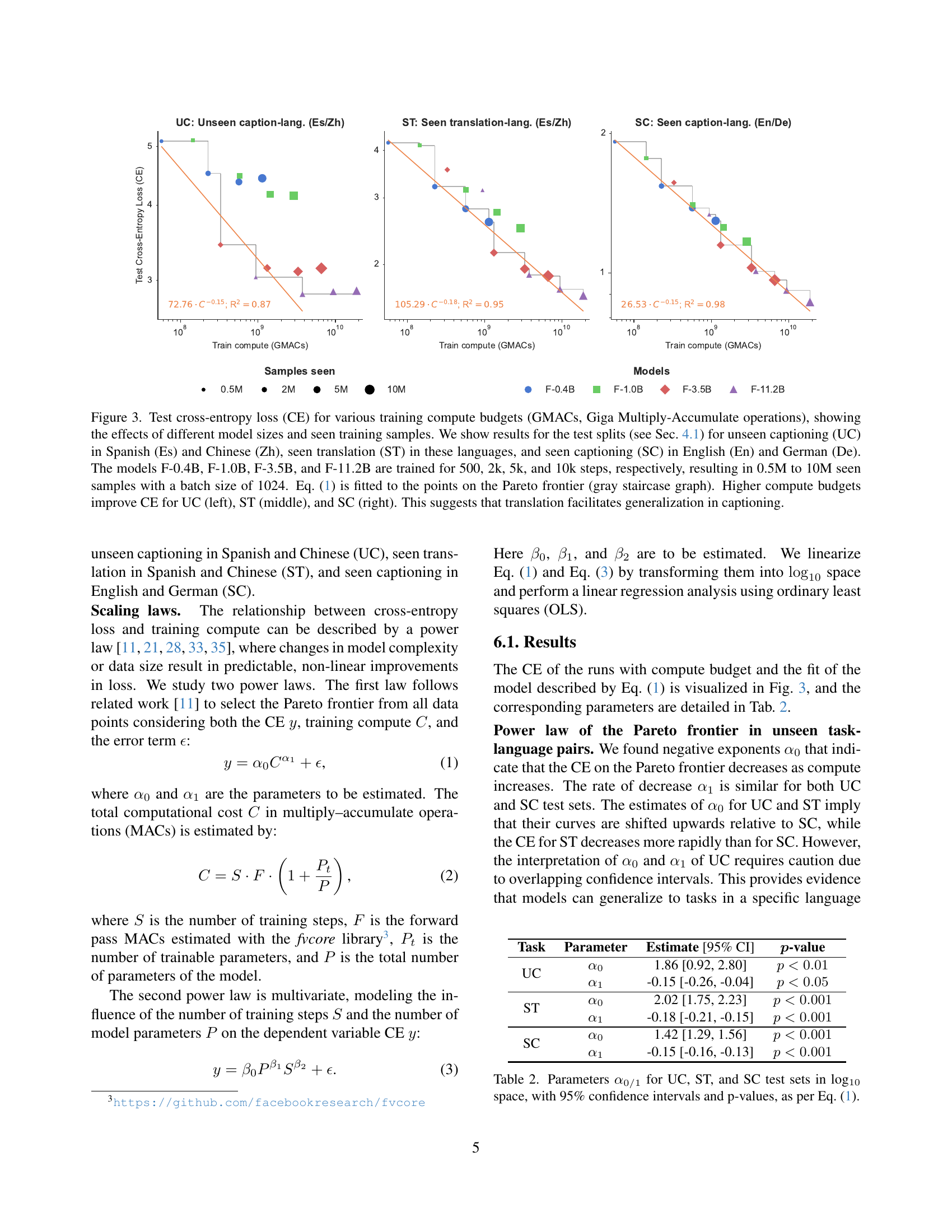
🔼 This figure displays the relationship between training compute (measured in Giga Multiply-Accumulate operations or GMACs), model size, and the cross-entropy loss (CE) for various tasks. Three different test sets are included: unseen captioning (UC) in Spanish and Chinese, seen translation (ST) in the same languages, and seen captioning (SC) in English and German. The results illustrate how increasing the compute budget and model size impacts the performance of each task. The gray staircase lines in each plot depict the Pareto frontier – the optimal tradeoff between compute and loss. The results suggest that having seen translation data helps the model generalize to unseen captioning tasks in new languages.
read the caption
Figure 3: Test cross-entropy loss (CE) for various training compute budgets (GMACs, Giga Multiply-Accumulate operations), showing the effects of different model sizes and seen training samples. We show results for the test splits (see Sec. 4.1) for unseen captioning (UC) in Spanish (Es) and Chinese (Zh), seen translation (ST) in these languages, and seen captioning (SC) in English (En) and German (De). The models F-0.4B, F-1.0B, F-3.5B, and F-11.2B are trained for 500, 2k, 5k, and 10k steps, respectively, resulting in 0.5M to 10M seen samples with a batch size of 1024. Eq. 1 is fitted to the points on the Pareto frontier (gray staircase graph). Higher compute budgets improve CE for UC (left), ST (middle), and SC (right). This suggests that translation facilitates generalization in captioning.

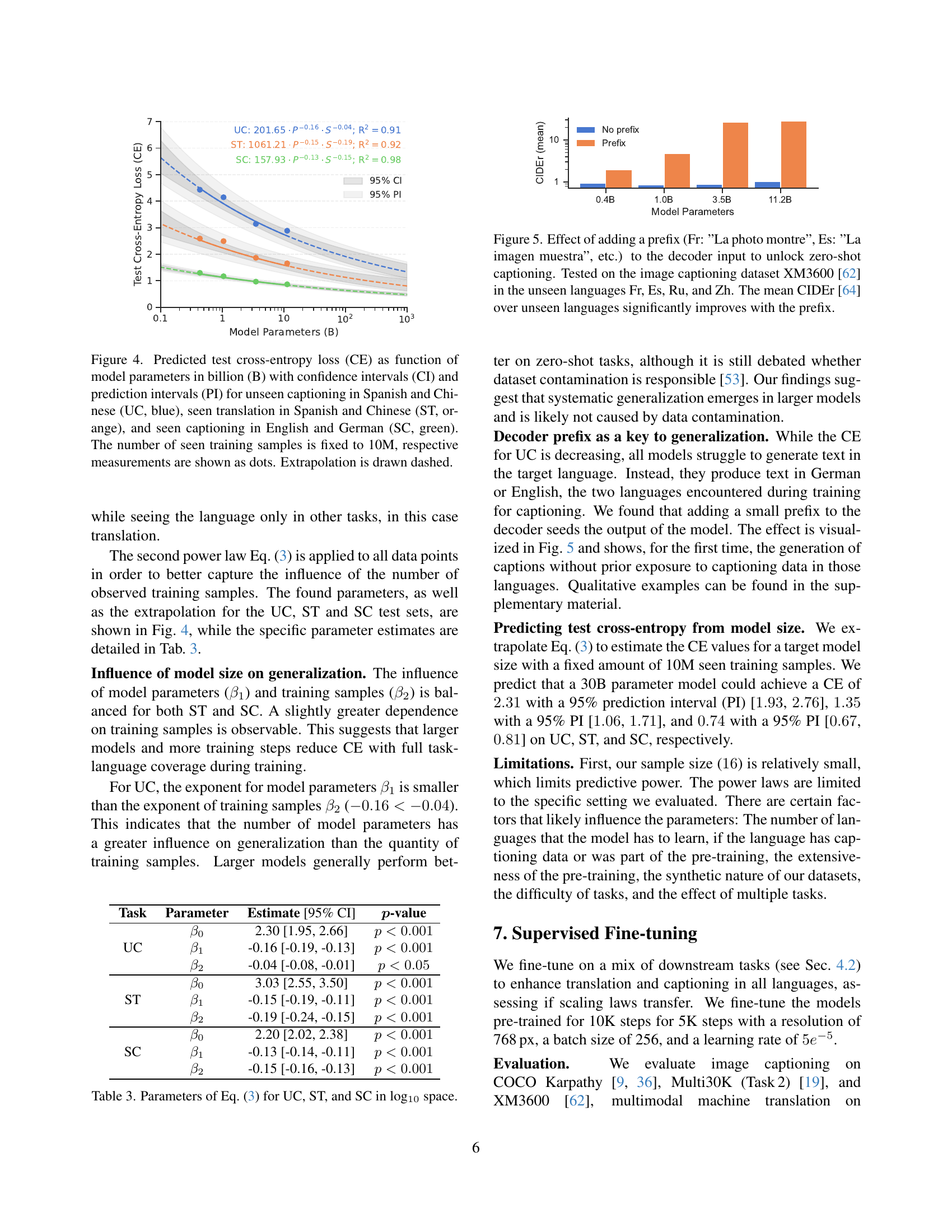
🔼 Figure 4 illustrates the scaling law relationship between model size and cross-entropy loss for three distinct scenarios. The y-axis shows the cross-entropy loss (a measure of model error), while the x-axis represents model size in billions of parameters. The three scenarios are: (1) unseen captioning tasks in Spanish and Chinese (UC, blue), representing the ability of a model to generate image captions in languages not encountered during training; (2) seen translation tasks in Spanish and Chinese (ST, orange), where the model has already seen translation tasks involving these languages during training; and (3) seen captioning tasks in English and German (SC, green), representing the model’s performance in languages it has seen extensively during training. The number of training samples was held constant at 10 million for all scenarios. The plot includes confidence intervals (CI) and prediction intervals (PI) to indicate the uncertainty associated with the estimates. The dashed lines represent extrapolations to larger model sizes.
read the caption
Figure 4: Predicted test cross-entropy loss (CE) as function of model parameters in billion (B) with confidence intervals (CI) and prediction intervals (PI) for unseen captioning in Spanish and Chinese (UC, blue), seen translation in Spanish and Chinese (ST, orange), and seen captioning in English and German (SC, green). The number of seen training samples is fixed to 10M, respective measurements are shown as dots. Extrapolation is drawn dashed.

🔼 This figure demonstrates how adding a language-specific prefix to the decoder input of a vision-language model (VLM) significantly improves its zero-shot image captioning capabilities in unseen languages. The experiment uses the XM3600 dataset [62], testing the model’s performance in French (Fr), Spanish (Es), Russian (Ru), and Chinese (Zh) – languages the model was not trained on for image captioning. The results, measured by CIDEr score [64], show a substantial increase when using prefixes, highlighting the effectiveness of this simple technique to enhance cross-lingual generalization in VLMs.
read the caption
Figure 5: Effect of adding a prefix (Fr: ”La photo montre”, Es: ”La imagen muestra”, etc.) to the decoder input to unlock zero-shot captioning. Tested on the image captioning dataset XM3600 [62] in the unseen languages Fr, Es, Ru, and Zh. The mean CIDEr [64] over unseen languages significantly improves with the prefix.

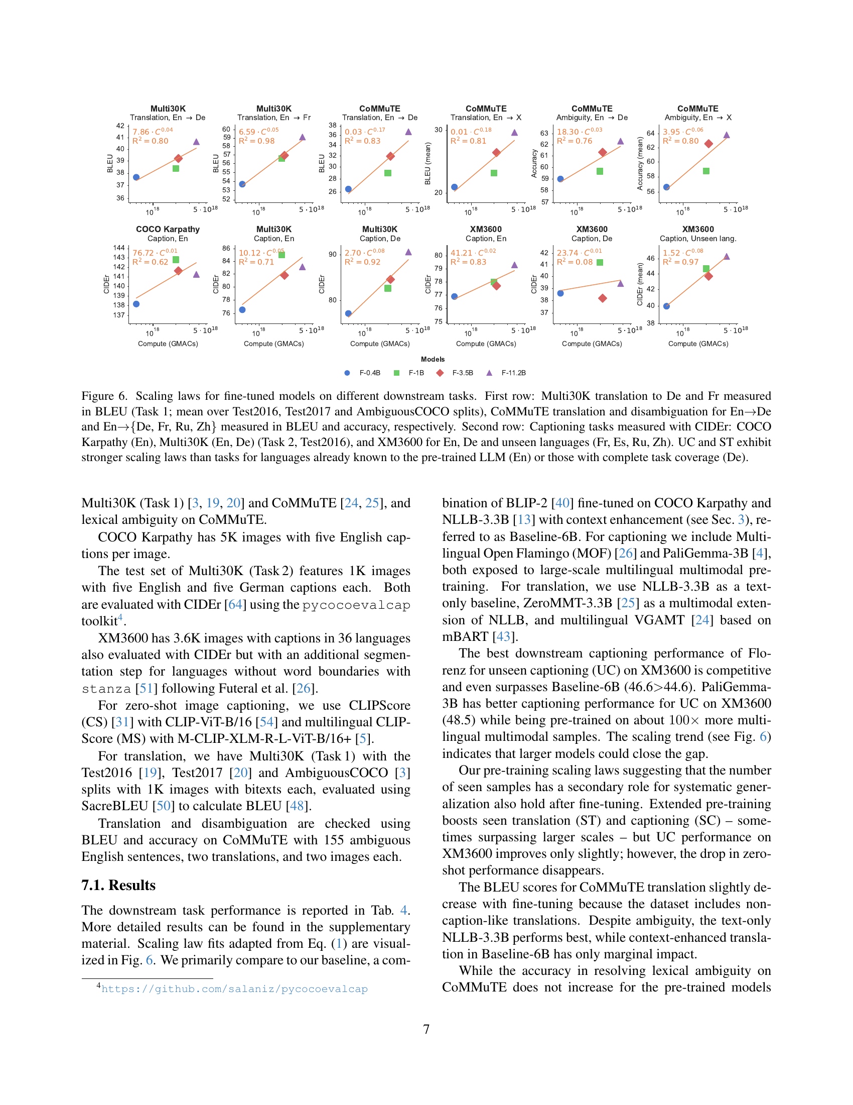
🔼 This figure displays the scaling laws observed when fine-tuning various sized vision-language models on multiple downstream tasks. The top row shows results for translation tasks from English to German (De) and French (Fr) using the Multi30K dataset, and for translation and disambiguation tasks using the CoMMuTE dataset (English to German, and English to German, French, Russian, and Chinese). The metric used is BLEU score for translation. The bottom row presents results for image captioning tasks, utilizing the CIDEr metric. Datasets include COCO Karpathy (English only), Multi30K (English and German), and XM3600 (English, German, and four other unseen languages: French, Spanish, Russian, and Chinese). The figure highlights that the scaling laws are stronger for tasks and languages that were either already familiar to the pre-trained language model (English) or had complete training data coverage (German), compared to those with limited data or unseen languages.
read the caption
Figure 6: Scaling laws for fine-tuned models on different downstream tasks. First row: Multi30K translation to De and Fr measured in BLEU (Task 1; mean over Test2016, Test2017 and AmbiguousCOCO splits), CoMMuTE translation and disambiguation for En→→\rightarrow→De and En→→\rightarrow→{De, Fr, Ru, Zh} measured in BLEU and accuracy, respectively. Second row: Captioning tasks measured with CIDEr: COCO Karpathy (En), Multi30K (En, De) (Task 2, Test2016), and XM3600 for En, De and unseen languages (Fr, Es, Ru, Zh). UC and ST exhibit stronger scaling laws than tasks for languages already known to the pre-trained LLM (En) or those with complete task coverage (De).

🔼 This figure shows a breakdown of the language coverage in the pre-training dataset used to train the Florenz model. It visually represents the proportions of caption and translation data available for each language, highlighting the imbalance in data distribution across different languages.
read the caption
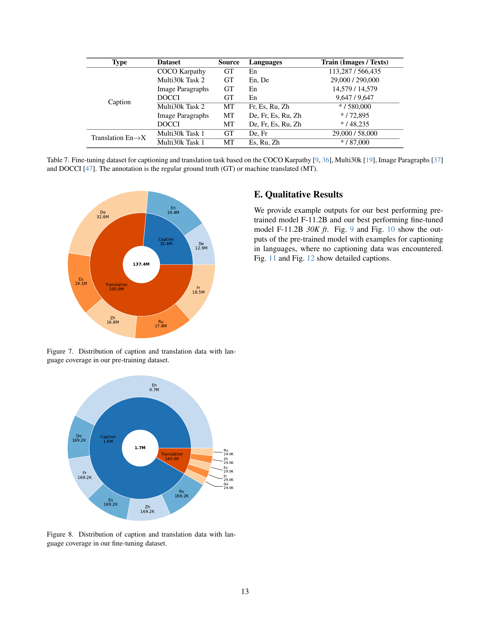
Figure 7: Distribution of caption and translation data with language coverage in our pre-training dataset.

🔼 This figure shows a breakdown of the language coverage in the fine-tuning dataset used for the Florenz model. It visually represents the proportion of caption and translation data available for each language, illustrating which languages have more extensive data for both captioning and translation tasks, and which languages have a more limited dataset.
read the caption
Figure 8: Distribution of caption and translation data with language coverage in our fine-tuning dataset.

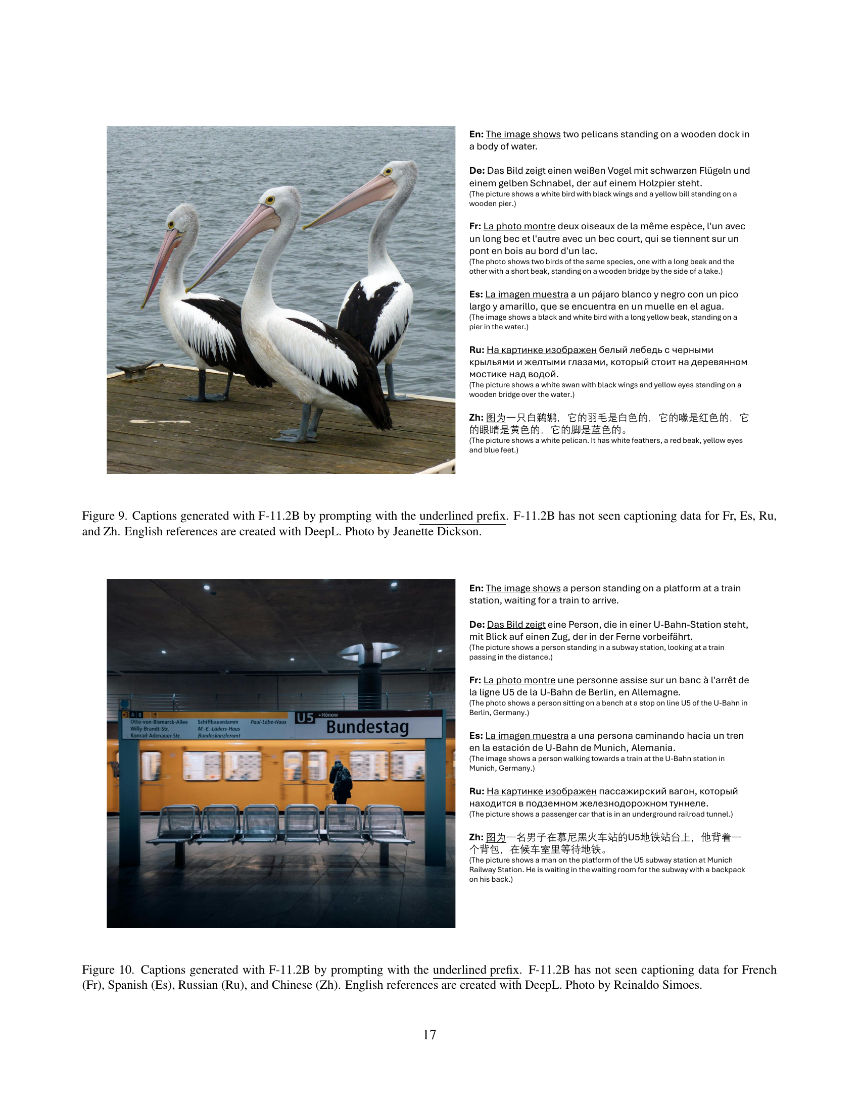
🔼 Figure 9 shows example captions generated by the F-11.2B model (a large vision-language model) in four different languages: French (Fr), Spanish (Es), Russian (Ru), and Chinese (Zh). Crucially, this model had not received any training data for image captioning in these languages. The captions were generated by providing the model with a short prompt (the underlined prefix in the figure). The English translations of the generated captions are also provided for comparison and were created using the DeepL translation service. The image used is a photo of three pelicans on a dock.
read the caption
Figure 9: Captions generated with F-11.2B by prompting with the underlined prefix. F-11.2B has not seen captioning data for Fr, Es, Ru, and Zh. English references are created with DeepL. Photo by Jeanette Dickson.

🔼 Figure 10 shows example captions generated by the F-11.2B model (one of the Florenz models) for an image depicting a person at a train station. Crucially, the model had not been trained on captioning data for French, Spanish, Russian, or Chinese. The model was prompted with a prefix in each language (underlined in the figure) before generating the caption in that language. The English captions provided are machine translations created with DeepL.
read the caption
Figure 10: Captions generated with F-11.2B by prompting with the underlined prefix. F-11.2B has not seen captioning data for French (Fr), Spanish (Es), Russian (Ru), and Chinese (Zh). English references are created with DeepL. Photo by Reinaldo Simoes.

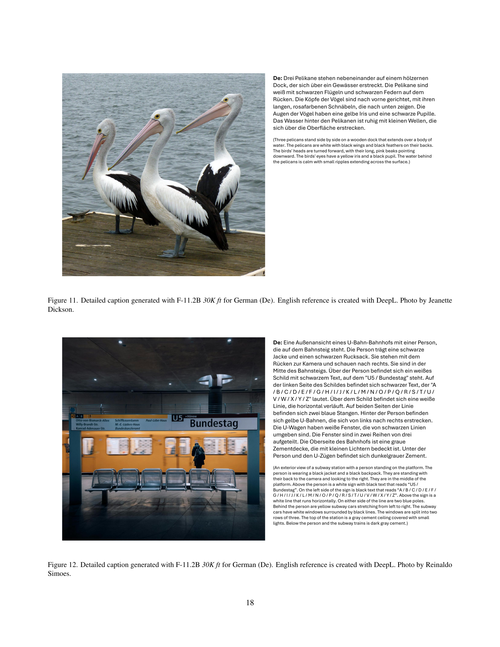
🔼 Figure 11 shows a detailed caption generated by the F-11.2B 30K ft model for a picture of three pelicans standing on a dock. The caption is in German. An English translation, created using DeepL, is also provided for comparison and better understanding. The photo itself was taken by Jeanette Dickson.
read the caption
Figure 11: Detailed caption generated with F-11.2B 30K ft for German (De). English reference is created with DeepL. Photo by Jeanette Dickson.

🔼 Figure 12 shows a detailed caption generated by the F-11.2B 30K ft model for a German-language image. The image depicts a person at a train station. The model generated a lengthy, highly descriptive caption of the scene in German. An English translation is included for comparison, generated using the DeepL translation service. The photograph is credited to Reinaldo Simoes.
read the caption
Figure 12: Detailed caption generated with F-11.2B 30K ft for German (De). English reference is created with DeepL. Photo by Reinaldo Simoes.

More on tables

Task	Parameter	Estimate [95% CI]	$\bm{p}$ -value
UC	$\alpha_{0}$	1.86 [0.92, 2.80]	$p<0.01$
UC	$\alpha_{1}$	-0.15 [-0.26, -0.04]	$p<0.05$
ST	$\alpha_{0}$	2.02 [1.75, 2.23]	$p<0.001$
ST	$\alpha_{1}$	-0.18 [-0.21, -0.15]	$p<0.001$
SC	$\alpha_{0}$	1.42 [1.29, 1.56]	$p<0.001$
SC	$\alpha_{1}$	-0.15 [-0.16, -0.13]	$p<0.001$

🔼 This table presents the results of fitting a power-law model (Equation 1 in the paper) to the relationship between cross-entropy loss and training compute. The model’s parameters (α0 and α1) are shown, along with 95% confidence intervals and p-values, indicating the statistical significance of the results. Three test sets are included: UC (Unseen caption-language), ST (Seen translation-language), and SC (Seen caption-language). The log10 space transformation is used for the compute and loss values. The parameters provide insights into how well the power law fits the data and how the cross-entropy loss changes as computational resources used for training are increased.
read the caption
Table 2: Parameters α0/1subscript𝛼01\alpha_{0/1}italic_α start_POSTSUBSCRIPT 0 / 1 end_POSTSUBSCRIPT for UC, ST, and SC test sets in log10 space, with 95% confidence intervals and p-values, as per Eq. 1.

Task	Parameter	Estimate [95% CI]	$\bm{p}$ -value
UC	$\beta_{0}$	2.30 [1.95, 2.66]	$p<0.001$
	$\beta_{1}$	-0.16 [-0.19, -0.13]	$p<0.001$
	$\beta_{2}$	-0.04 [-0.08, -0.01]	$p<0.05$
ST	$\beta_{0}$	3.03 [2.55, 3.50]	$p<0.001$
	$\beta_{1}$	-0.15 [-0.19, -0.11]	$p<0.001$
	$\beta_{2}$	-0.19 [-0.24, -0.15]	$p<0.001$
SC	$\beta_{0}$	2.20 [2.02, 2.38]	$p<0.001$
	$\beta_{1}$	-0.13 [-0.14, -0.11]	$p<0.001$
	$\beta_{2}$	-0.15 [-0.16, -0.13]	$p<0.001$

🔼 This table presents the results of a multivariate power law analysis, modeling the influence of model parameters and the number of training steps on the cross-entropy loss (CE). The analysis was performed for three different test settings: unseen captioning (UC), seen translation (ST), and seen captioning (SC). The table displays the estimated parameters (β0, β1, β2) and their 95% confidence intervals (CI) for each test setting, along with p-values indicating statistical significance. The parameters quantify the relationship between the model size, training data, and the resulting cross-entropy loss in a log10 space.
read the caption
Table 3: Parameters of Eq. 3 for UC, ST, and SC in log10 space.

	Multi30K		CoMMuTE		CoMMuTE		COCO	Multi30K		XM3600
	Translation		Translation		Ambiguity		Caption	Caption		Caption
	En $\rightarrow$ De	En $\rightarrow$ Fr	En $\rightarrow$ De	En $\rightarrow$ X	En $\rightarrow$ De	En $\rightarrow$ X	En	En	De	En	De	Unseen
Supervised
Model	BLEU	BLEU	BLEU	BLEU	Acc.	Acc.	CIDEr	CIDEr	CIDEr	CIDEr	CIDEr	CIDEr
VGAMT [24]	37.4	58.4			57.1
Florence-2-large [69]							143.3
PaliGemma-3B* [4]							141.7	88.9	57.6	79.1	37.7	48.5
Baseline-6B* [40, 13]	37.3	54.3	41.5	32.5	61.7	61.1	145.2	84.0	50.4	82.0	38.2	45.1
F-0.4B ft (ours)	37.7	53.7	26.5	20.8	59.0	56.6	138.2	76.6	77.4	76.9	38.6	40.0
F-0.4B 100K ft (ours)	39.9	57.2	32.8	26.6	59.7	59.8	140.3	79.5	79.2	78.3	39.3	42.0
F-1.0B ft (ours)	38.4	56.6	29.0	22.8	59.7	58.8	142.8	85.1	82.6	78.0	41.2	44.7
F-3.5B ft (ours)	39.2	56.9	32.0	26.0	61.3	62.6	141.6	81.8	84.5	77.7	38.2	43.7
F-11.2B ft (ours)	40.7	59.1	36.8	29.6	62.3	63.9	141.3	83.1	90.7	79.3	39.4	46.3
F-11.2B 30K ft (ours)	41.7	59.6	38.5	31.2	62.0	63.4	140.8	83.4	89.4	78.1	41.8	46.9
Zero-shot
Model	BLEU	BLEU	BLEU	BLEU	Acc.	Acc.	CS	CS	MCS	CS	MCS	PC
MOF [26]	24.9	35.1			63.7	66.5
ZeroMMT-3.3B [25]	37.1	53.3			60.8	62.2
NLLB-3.3B* [13]	37.4	53.7	40.8	31.9	50.0	50.0
F-0.4B (ours)	34.1	44.3	34.1	25.9	54.0	53.6	77.7	77.9	82.0	74.8	77.1	1.7
F-0.4B 100K (ours)	36.1	51.0	37.2	29.5	54.0	54.2	77.9	78.2	83.3	75.4	78.3	1.8
F-1.0B (ours)	35.3	47.4	35.4	27.1	54.7	54.1	79.9	80.2	86.5	77.0	81.4	5.6
F-3.5B (ours)	35.8	48.3	36.7	28.7	53.0	54.3	78.5	78.7	83.7	75.9	79.5	24.1
F-11.2B (ours)	36.6	50.9	39.5	29.8	52.7	53.5	78.9	79.0	84.7	76.3	80.1	26.6
F-11.2B 30K (ours)	37.6	52.3	39.4	30.4	52.0	53.2	79.0	79.2	85.1	76.6	80.5	17.7

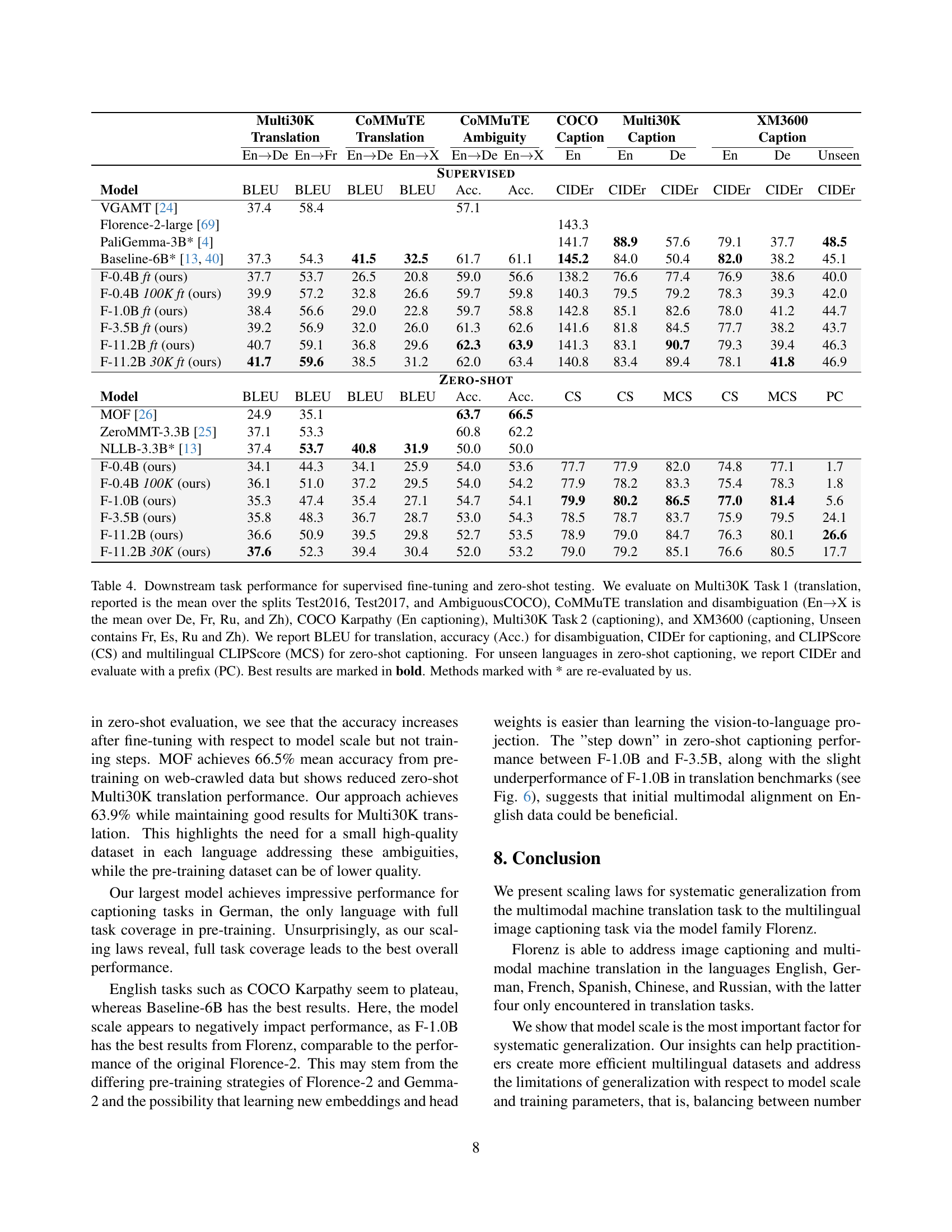
🔼 This table presents a comprehensive evaluation of different vision-language models (VLMs) across various downstream tasks, comparing their performance under both supervised fine-tuning and zero-shot settings. The tasks include translation (Multi30K, CoMMuTE), lexical disambiguation (CoMMuTE), and image captioning (COCO Karpathy, Multi30K, XM3600). Evaluation metrics vary by task and include BLEU score for translation, accuracy for disambiguation, and CIDEr score and CLIPScore (both standard and multilingual versions) for image captioning. The results highlight the models’ ability to generalize to unseen languages and tasks, particularly in the zero-shot setting when a text prefix is used. The table shows several models’ performances, including some re-evaluated baselines and the authors’ proposed models in different sizes. The best performances are highlighted.
read the caption
Table 4: Downstream task performance for supervised fine-tuning and zero-shot testing. We evaluate on Multi30K Task 1 (translation, reported is the mean over the splits Test2016, Test2017, and AmbiguousCOCO), CoMMuTE translation and disambiguation (En→→\rightarrow→X is the mean over De, Fr, Ru, and Zh), COCO Karpathy (En captioning), Multi30K Task 2 (captioning), and XM3600 (captioning, Unseen contains Fr, Es, Ru and Zh). We report BLEU for translation, accuracy (Acc.) for disambiguation, CIDEr for captioning, and CLIPScore (CS) and multilingual CLIPScore (MCS) for zero-shot captioning. For unseen languages in zero-shot captioning, we report CIDEr and evaluate with a prefix (PC). Best results are marked in bold. Methods marked with * are re-evaluated by us.

	Florenz (F)
Param.	0.4B	1B	3.5B	11.2B
	Vision Encoder
	DaViT [16]
# layers	[1, 1, 9, 1]	[1, 1, 9, 1]
Hidden dim.	[128, 256, 512, 1024]	[256, 512, 1024, 2048]
# heads	[4, 8, 16, 32]	[8, 16, 32, 64]
Patch size	[7, 3, 3, 3]	[7, 3, 3, 3]
Patch stride	[4, 2, 2, 2]	[4, 2, 2, 2]
	Encoder
	Florence-2 [69]
# layers	6	12
Hidden dim.	768	1024
# heads	12	16
Vocab. size	51328
	Decoder
	Florence-2 [69]		Gemma-2 [61]
# layers	6	12	26	42
Hidden dim.	768	1024	2304	3584
# heads	12	16	8	16
Vocab. size	256000

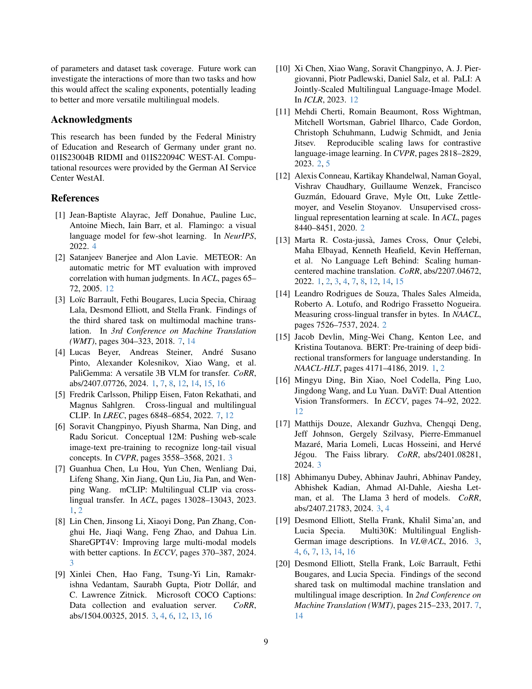
🔼 This table details the architecture of the Florenz model family, which consists of various sizes (0.4B, 1B, 3.5B, and 11.2B parameters). It breaks down the model components (vision encoder and decoder) and their respective configurations, including the number of layers, hidden dimensions, number of attention heads, patch size and stride for the vision encoder, and vocabulary size for the decoder. The table clarifies the specific pre-trained models used for each component, highlighting the combination of Florence-2 (vision) and Gemma-2 (language).
read the caption
Table 5: Model configuration of Florenz.

Model	En	De	Fr	Es	Ru	Zh
Paper [4]	78.0	-	-	-	-	-
Reprod.	78.4	35.6	63.6	68.0	35.3	28.4
stanza [51]	78.7	35.9	63.2	67.9	35.6	28.2
Baseline-6B [40, 13]	81.9	38.1	64.9	63.9	29.4	21.5

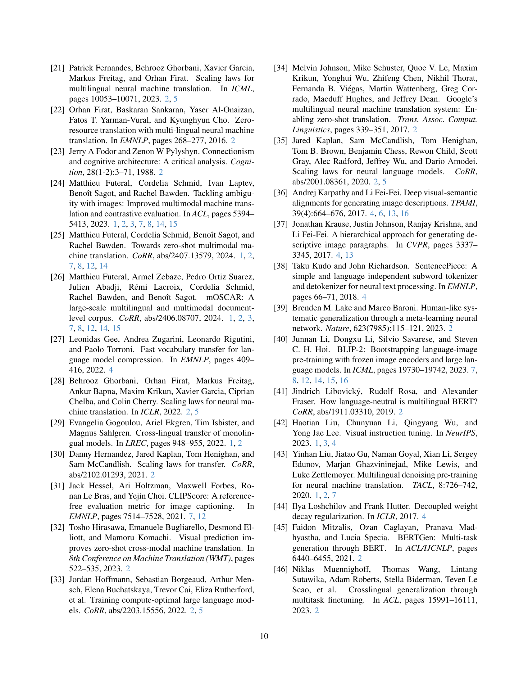
🔼 This table compares the CIDEr scores for image captioning on the XM3600 dataset across different models. The models compared include PaliGemma [4] (with its original pre-segmented outputs and a reproduction using stanza [51] for word segmentation), and the Baseline-6B model. This comparison highlights the impact of pre-segmentation and provides context for understanding the results reported in the paper.
read the caption
Table 6: Comparison between the numbers reported in the PaliGemma paper [4], reproduction with pre-segmented model outputs, reproduction with stanza [51] for word segmentation, and the Baseline-6B model for reference. Note that the outputs of PaliGemma-3B are pre-segmented, with words separated by whitespace. For the stanza evaluation, we first remove the whitespace before processing.

Type	Dataset	Source	Languages	Train (Images / Texts)
Caption	COCO Karpathy	GT	En	113,287 / 566,435
	Multi30k Task 2	GT	En, De	29,000 / 290,000
	Image Paragraphs	GT	En	14,579 / 14,579
	DOCCI	GT	En	9,647 / 9,647
	Multi30k Task 2	MT	Fr, Es, Ru, Zh	* / 580,000
	Image Paragraphs	MT	De, Fr, Es, Ru, Zh	* / 72,895
	DOCCI	MT	De, Fr, Es, Ru, Zh	* / 48,235
Translation En $\rightarrow$ X	Multi30k Task 1	GT	De, Fr	29,000 / 58,000
Translation En $\rightarrow$ X	Multi30k Task 1	MT	Es, Ru, Zh	* / 87,000

🔼 This table details the composition of the fine-tuning dataset used in the experiments. It breaks down the data by task (captioning or translation), dataset source (COCO Karpathy, Multi30k, Image Paragraphs, or DOCCI), language(s) included, and the number of images and texts. The annotation type is specified as either ground truth (GT) or machine translated (MT). This dataset is a mix of several publicly available resources augmented with machine translation for languages missing data in the original resources.
read the caption
Table 7: Fine-tuning dataset for captioning and translation task based on the COCO Karpathy [9, 36], Multi30k [19], Image Paragraphs [37] and DOCCI [47]. The annotation is the regular ground truth (GT) or machine translated (MT).

Multi30K Translation En $\rightarrow$ Fr
		Test2016		Test2017		Test2018		COCO
	Model	B	C₂₂	B	C₂₂	B	C₂₂	B	C₂₂
supervised	VGAMT [24]	65.0	88.7	58.9	88.2			51.2	84.8
	Baseline-6B [40, 4]	54.8	87.6	53.8	87.6	45.7	84.8	54.4	85.6
	F-0.4B ft (ours)	57.5	85.9	53.5	85.9	39.6	82.3	50.0	82.4
	F-0.4B 100k ft (ours)	60.4	87.7	57.5	87.9	43.0	84.0	53.8	84.7
	F-1.0B ft (ours)	59.9	87.5	56.9	87.3	42.4	83.5	52.9	84.2
	F-3.5B ft (ours)	59.9	88.5	57.5	88.4	42.2	84.2	53.5	85.2
	F-11.2B ft (ours)	63.2	89.2	60.3	89.1	43.9	84.9	53.9	85.8
	F-11.2B 30K ft (ours)	64.4	89.5	60.5	89.0	44.6	85.1	53.8	86.1
text	NLLB-600M [13]	48.3	85.0	48.5	85.9	40.5	83.0	50.0	84.1
	NLLB-1.3B [13]	51.8	86.6	50.9	86.9	43.0	84.1	52.8	85.0
	NLLB-3.3B [13]	54.2	87.6	52.8	87.5	45.4	84.8	54.1	85.6
zero-shot	MOF [26]	36.0	83.6	35.1	83.7			34.1	80.7
	ZeroMMT-600M [25]	48.6	84.9	48.1	85.7			50.3	83.8
	ZeroMMT-1.3B [25]	51.5	86.4	51.1	87.0			53.6	85.0
	ZeroMMT-3.3B [25]	52.9	87.2	53.3	87.5			53.9	85.4
	F-0.4B (ours)	42.1	81.6	43.4	82.1	36.2	79.6	47.6	80.4
	F-0.4B 100K (ours)	49.0	85.0	50.1	85.9	42.2	83.1	53.9	83.7
	F-1.0B (ours)	45.3	83.6	46.3	84.4	39.1	82.0	50.7	82.0
	F-3.5B (ours)	46.5	85.1	48.0	85.8	40.3	83.1	50.5	83.1
	F-11.2B (ours)	50.6	86.0	50.2	86.7	42.2	83.6	52.0	84.4
	F-11.2B 30K (ours)	51.3	86.1	51.4	87.0	43.4	83.8	54.3	84.9
Multi30K Translation En $\rightarrow$ De
supervised	VGAMT [24]	41.9	85.8	36.7	84.7			33.5	81.1
	Baseline-6B [40, 4]	39.8	86.2	38.3	85.5	35.6	84.3	33.9	82.1
	F-0.4B ft (ours)	42.8	84.5	37.8	84.0	34.6	82.4	32.4	79.6
	F-0.4B 100K ft (ours)	44.0	86.3	40.9	86.1	36.5	84.1	34.8	82.1
	F-1.0B ft (ours)	43.2	85.9	38.7	85.3	35.7	83.7	33.3	80.8
	F-3.5B ft (ours)	43.1	86.6	39.8	85.9	36.8	84.4	34.7	82.0
	F-11.2B ft (ours)	44.7	87.3	41.6	87.0	37.7	85.4	35.7	83.6
	F-11.2B 30K ft (ours)	44.9	87.6	41.6	87.0	38.8	85.6	38.5	83.9
text	NLLB-600M [13]	37.2	83.5	33.0	83.0	32.2	81.9	28.3	78.6
	NLLB-1.3B [13]	38.1	85.0	36.7	84.3	32.8	83.2	31.5	80.4
	NLLB-3.3B [13]	39.7	86.1	37.9	85.2	35.8	84.2	34.5	82.0
zero-shot	MOF [26]	28.9	82.3	23.9	80.9			21.9	76.6
	ZeroMMT-600M [25]	36.2	83.0	33.2	82.5			29.0	77.7
	ZeroMMT-1.3B [25]	37.6	84.0	36.2	84.6			31.7	80.7
	ZeroMMT-3.3B [25]	39.6	85.9	37.9	85.5			33.7	81.9
	F-0.4B (ours)	37.2	83.1	35.9	83.6	32.9	81.9	29.3	78.4
	F-0.4B 100K (ours)	39.5	85.0	37.1	84.7	34.7	83.1	31.8	80.5
	F-1.0B (ours)	38.8	84.3	36.3	84.3	34.6	83.0	30.6	79.1
	F-3.5B (ours)	38.2	84.7	37.2	84.6	34.5	83.4	31.8	80.8
	F-11.2B (ours)	39.3	85.7	37.7	85.4	34.6	83.9	32.7	81.1
	F-11.2B 30K (ours)	39.5	85.8	38.3	85.4	36.0	84.1	35.0	81.6

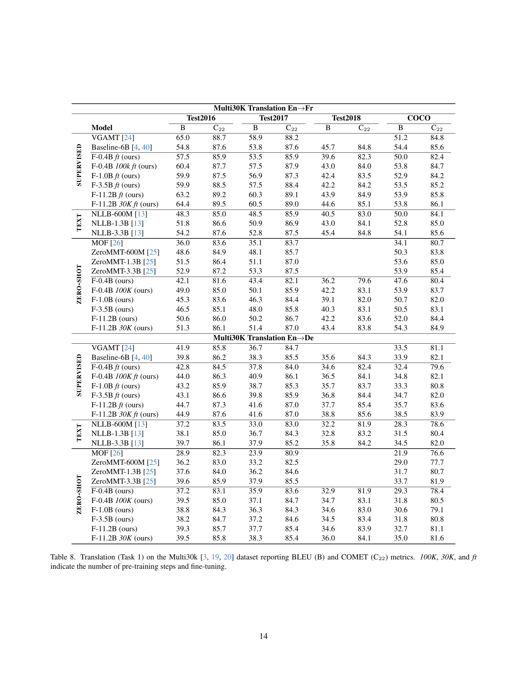
🔼 Table 8 presents the results of the Multi30K translation task (Task 1), specifically focusing on English-to-German and English-to-French translations. The table evaluates performance using two metrics: BLEU (B), a widely used automatic metric for machine translation quality, and COMET (C22), a more recent metric that attempts to better correlate with human judgments of fluency and adequacy. Different model configurations are compared. The ‘100K’, ‘30K’, and ‘ft’ columns indicate the number of pre-training steps and whether fine-tuning was performed, providing insight into the impact of training on translation quality.
read the caption
Table 8: Translation (Task 1) on the Multi30k [19, 20, 3] dataset reporting BLEU (B) and COMET (C22) metrics. 100K, 30K, and ft indicate the number of pre-training steps and fine-tuning.

	De		Fr		Ru		Zh
Model	B	C₂₂	B	C₂₂	B	C₂₂	B	C₂₂
NLLB-600M [13]	36.4	80.6	38.9	80.2	19.8	80.1	20.8	75.5
NLLB-1B [13]	40.5	81.3	39.2	80.4	23.7	81.9	20.3	75.6
NLLB-3.3B [13]	40.8	81.3	41.4	81.4	22.7	82.4	22.8	77.0
Baseline-6B [40, 4]	41.5	81.6	42.1	81.5	23.5	82.9	23.0	77.2
F-0.4B ft (ours)	26.5	71.6	27.8	72.9	9.9	69.2	19.1	73.1
F-0.4B 100K ft (ours)	32.8	78.3	37.6	78.6	13.6	77.5	22.5	75.0
F-1.0B ft (ours)	29.0	74.3	30.5	75.4	12.0	72.7	19.5	74.3
F-3.5B ft (ours)	32.0	79.3	35.5	78.6	15.0	77.9	21.5	75.2
F-11.2B ft (ours)	36.8	81.5	40.7	81.3	18.1	80.9	22.7	75.4
F-11.2B 30K ft (ours)	38.5	82.4	42.6	81.9	19.6	81.3	23.9	76.6
F-0.4B (ours)	34.1	77.5	31.0	76.4	12.5	71.1	26.2	76.6
F-0.4B 100K (ours)	37.2	80.4	37.4	78.5	16.4	77.7	27.1	77.8
F-1.0B (ours)	35.4	78.8	32.4	77.0	14.2	75.5	26.2	77.1
F-3.5B (ours)	36.7	80.0	36.8	78.1	14.6	79.1	26.9	77.7
F-11.2B (ours)	39.5	80.7	37.5	79.1	16.1	79.2	26.3	76.6
F-11.2B 30K (ours)	39.4	80.5	35.8	78.8	17.6	78.8	28.6	77.4

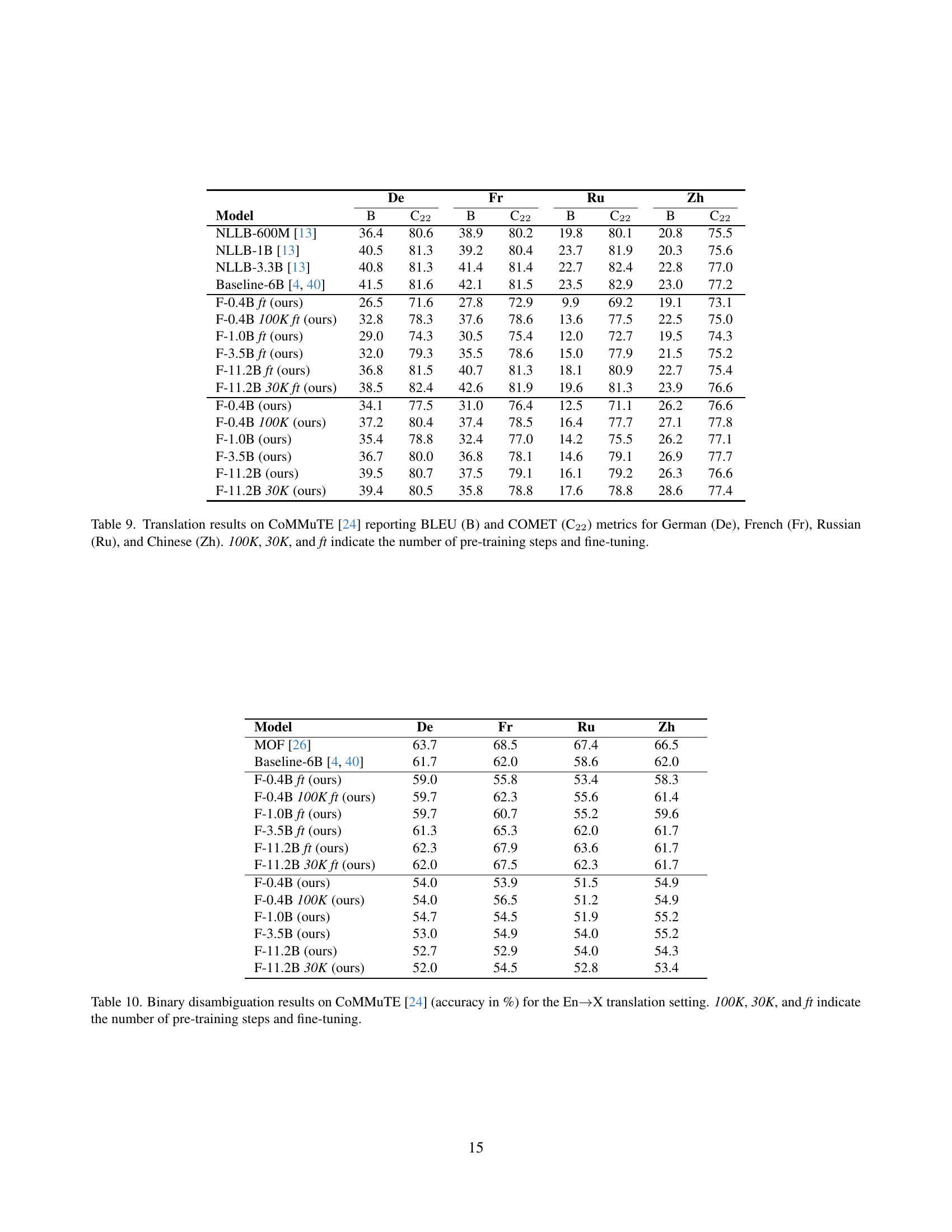
🔼 This table presents the results of machine translation experiments conducted on the CoMMuTE dataset [24]. The experiments evaluated the performance of various models, including different versions of the Florenz model family (with varying numbers of parameters and training steps), along with established baselines. The evaluation metrics used were BLEU (B) and COMET (C22), two common machine translation evaluation scores. The table shows scores for translations into four different languages: German (De), French (Fr), Russian (Ru), and Chinese (Zh). The ‘100K’, ‘30K’, and ‘ft’ notations in the table indicate the training procedure for each model, representing the number of pre-training steps and whether fine-tuning was applied. This table aims to demonstrate how various factors, such as model size and training methodology, influence the performance of cross-lingual translation.
read the caption
Table 9: Translation results on CoMMuTE [24] reporting BLEU (B) and COMET (C22) metrics for German (De), French (Fr), Russian (Ru), and Chinese (Zh). 100K, 30K, and ft indicate the number of pre-training steps and fine-tuning.

Model	De	Fr	Ru	Zh
MOF [26]	63.7	68.5	67.4	66.5
Baseline-6B [40, 4]	61.7	62.0	58.6	62.0
F-0.4B ft (ours)	59.0	55.8	53.4	58.3
F-0.4B 100K ft (ours)	59.7	62.3	55.6	61.4
F-1.0B ft (ours)	59.7	60.7	55.2	59.6
F-3.5B ft (ours)	61.3	65.3	62.0	61.7
F-11.2B ft (ours)	62.3	67.9	63.6	61.7
F-11.2B 30K ft (ours)	62.0	67.5	62.3	61.7
F-0.4B (ours)	54.0	53.9	51.5	54.9
F-0.4B 100K (ours)	54.0	56.5	51.2	54.9
F-1.0B (ours)	54.7	54.5	51.9	55.2
F-3.5B (ours)	53.0	54.9	54.0	55.2
F-11.2B (ours)	52.7	52.9	54.0	54.3
F-11.2B 30K (ours)	52.0	54.5	52.8	53.4

🔼 Table 10 presents the accuracy (in percentage) achieved in binary disambiguation tasks using the CoMMuTE dataset [24]. The experiment focuses on English-to-X translation, where ‘X’ represents various languages. The table showcases the performance of different Florenz models (with varying parameter counts and training stages) on this task. The ‘100K’, ‘30K’, and ‘ft’ notations in the table indicate the number of pre-training steps conducted on the model, and whether fine-tuning was applied, respectively. This allows for an analysis of the influence of both model scale and training procedures on the disambiguation task’s success.
read the caption
Table 10: Binary disambiguation results on CoMMuTE [24] (accuracy in %) for the En→→\rightarrow→X translation setting. 100K, 30K, and ft indicate the number of pre-training steps and fine-tuning.

	B@4	C	CS
supervised
PaliGemma-3B [4]	41.6	141.7	77.1
Florence-2-base [69]		140.0
Florence-2-large [69]		143.3
Baseline-6B [40, 4]	42.8	145.2	76.9
F-0.4B ft (ours)	40.6	138.2	76.2
F-0.4B 100K ft (ours)	41.3	140.3	76.6
F-1.0B ft (ours)	41.2	142.8	77.4
F-3.5B ft (ours)	41.8	141.6	76.6
F-11.2B ft (ours)	41.7	141.3	76.6
F-11.2B 30K ft (ours)	41.6	140.8	76.6
zero-shot
Florence-2-base	37.6	132.9	77.2
Florence-2-large	38.3	135.9	77.6
F-0.4B (ours)	13.2	28.2	77.7
F-0.4B 100K (ours)	12.7	27.3	77.9
F-1.0B (ours)	12.6	21.3	79.9
F-3.5B (ours)	13.3	28.7	78.5
F-11.2B (ours)	13.7	30.5	78.9
F-11.2B 30K (ours)	15.1	24.9	79.2

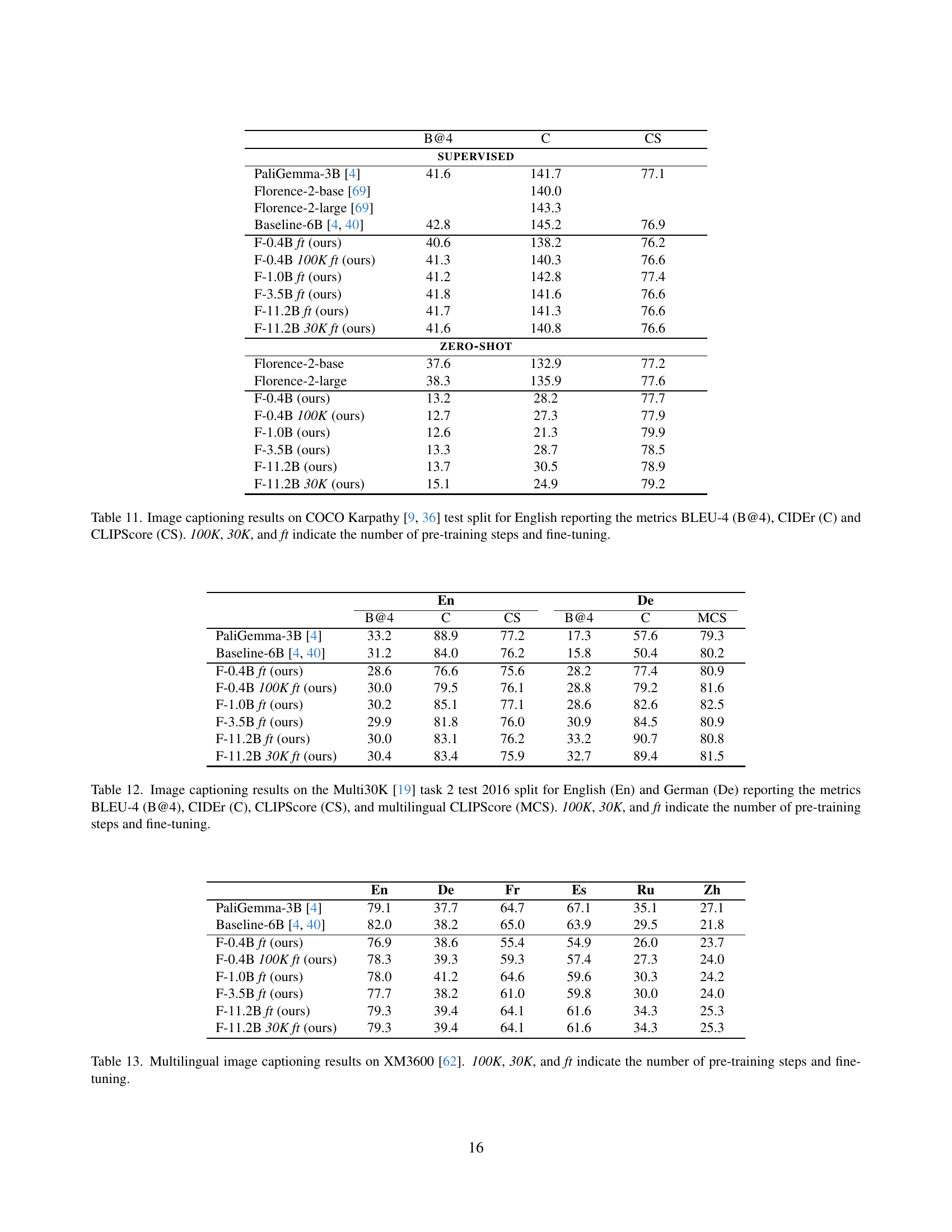
🔼 This table presents the performance of various models on the COCO Karpathy image captioning benchmark. The benchmark uses English captions. The results are reported using three metrics: BLEU-4 (B@4), CIDEr (C), and CLIPScore (CS). The table compares several models, including the Florence model family (with different parameter sizes and training/fine-tuning configurations), other state-of-the-art models (such as PaliGemma and Baseline-6B), and also shows results with and without fine-tuning. The numbers 100K, 30K, and ‘ft’ in the table indicate the number of pre-training steps and whether fine-tuning was performed. This allows for a comprehensive comparison of model performance across different scales and training strategies.
read the caption
Table 11: Image captioning results on COCO Karpathy [9, 36] test split for English reporting the metrics BLEU-4 (B@4), CIDEr (C) and CLIPScore (CS). 100K, 30K, and ft indicate the number of pre-training steps and fine-tuning.

	En			De
	B@4	C	CS	B@4	C	MCS
PaliGemma-3B [4]	33.2	88.9	77.2	17.3	57.6	79.3
Baseline-6B [40, 4]	31.2	84.0	76.2	15.8	50.4	80.2
F-0.4B ft (ours)	28.6	76.6	75.6	28.2	77.4	80.9
F-0.4B 100K ft (ours)	30.0	79.5	76.1	28.8	79.2	81.6
F-1.0B ft (ours)	30.2	85.1	77.1	28.6	82.6	82.5
F-3.5B ft (ours)	29.9	81.8	76.0	30.9	84.5	80.9
F-11.2B ft (ours)	30.0	83.1	76.2	33.2	90.7	80.8
F-11.2B 30K ft (ours)	30.4	83.4	75.9	32.7	89.4	81.5

🔼 This table presents the performance of various models on the Multi30K image captioning dataset. Specifically, it focuses on the English and German captions from the 2016 test split. The evaluation metrics used are BLEU-4 (B@4), CIDEr (C), CLIPScore (CS), and multilingual CLIPScore (MCS), providing a comprehensive assessment of the caption quality. The table includes results for both zero-shot and supervised fine-tuned models. The number of pre-training steps (100K, 30K) and whether fine-tuning (ft) was performed are indicated to allow for better comparison of different model training regimes.
read the caption
Table 12: Image captioning results on the Multi30K [19] task 2 test 2016 split for English (En) and German (De) reporting the metrics BLEU-4 (B@4), CIDEr (C), CLIPScore (CS), and multilingual CLIPScore (MCS). 100K, 30K, and ft indicate the number of pre-training steps and fine-tuning.

	En	De	Fr	Es	Ru	Zh
PaliGemma-3B [4]	79.1	37.7	64.7	67.1	35.1	27.1
Baseline-6B [40, 4]	82.0	38.2	65.0	63.9	29.5	21.8
F-0.4B ft (ours)	76.9	38.6	55.4	54.9	26.0	23.7
F-0.4B 100K ft (ours)	78.3	39.3	59.3	57.4	27.3	24.0
F-1.0B ft (ours)	78.0	41.2	64.6	59.6	30.3	24.2
F-3.5B ft (ours)	77.7	38.2	61.0	59.8	30.0	24.0
F-11.2B ft (ours)	79.3	39.4	64.1	61.6	34.3	25.3
F-11.2B 30K ft (ours)	79.3	39.4	64.1	61.6	34.3	25.3

🔼 Table 13 presents the results of multilingual image captioning on the XM3600 benchmark dataset [62]. The table shows the performance of various models, including different sizes of the Florenz model family (with varying pre-training steps), along with some baseline models for comparison. The evaluation metrics used are CIDEr scores for English, German, French, Spanish, Russian, and Chinese. The ‘100K’, ‘30K’, and ‘ft’ notations indicate the number of pre-training steps and whether fine-tuning was applied.
read the caption
Table 13: Multilingual image captioning results on XM3600 [62]. 100K, 30K, and ft indicate the number of pre-training steps and fine-tuning.

TL;DR#

Key Takeaways#

Why does it matter?#

Visual Insights#

In-depth insights#

Monolingual Scaling#

Florenz’s Design#

Synthetic Data#

Prefix Generalize#

Task Balance#

More visual insights#

Full paper#