TL;DR#
Diffusion models, while powerful for image generation, are computationally intensive, requiring many iterative denoising steps. Existing methods to speed up inference, like GAN-based approaches and consistency models (CMs), have limitations such as training instability and quality erosion in ultra-few-step regimes. These challenges hinder broader adoption, highlighting the need for a framework that balances efficiency, flexibility, and quality.
To solve the issues, the paper presents SANA-Sprint, an efficient diffusion model for ultra-fast text-to-image (T2I) generation. SANA-Sprint is built on a pre-trained foundation model and augmented with hybrid distillation, dramatically reducing inference steps. It introduces a training-free approach for continuous-time consistency distillation (sCM), combined with latent adversarial distillation (LADD) to enhance single-step generation fidelity. Integrated with ControlNet, SANA-Sprint enables real-time interactive image generation, achieving state-of-the-art performance in speed-quality tradeoffs.
Key Takeaways#
Why does it matter?#
SANA-Sprint is an efficient diffusion model for real-time text-to-image generation, enabling its potential for AI-powered consumer applications. The efficiency unlocks transformative applications that require instant visual feedback, making it suitable for human-in-the-loop creative workflows, AIPC, and immersive AR/VR interfaces.
Visual Insights#

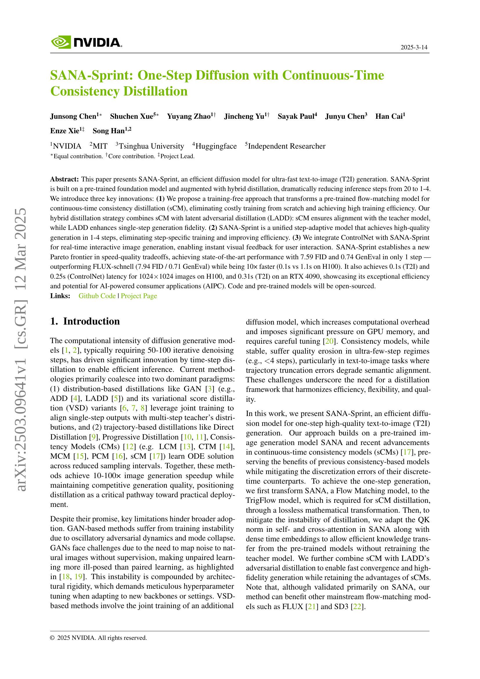
🔼 Figure 1 presents a comparison of SANA-Sprint’s performance against existing state-of-the-art models in terms of inference speed and GPU memory usage. The left panel (a) shows a dramatic speed improvement by SANA-Sprint, reducing the time to generate 1024x1024 images from 1.94 seconds (Flux-Schnell) to a mere 0.03 seconds – a 64x speedup. This improvement is calculated based on the time taken by the transformer components of the models, using a batch size of 1 on an NVIDIA A100 GPU. The right panel (b) demonstrates SANA-Sprint’s efficiency in terms of GPU memory usage during training, outperforming other distillation methods. The memory usage was measured using the official code and a single A100 GPU with 1024x1024 images.
read the caption
Figure 1: (a) Our SANA-Sprint accelerate the inference speed for generating 1024 ×\times× 1024 images, achieving a remarkable speedup from FULX-Schnell’s 1.94 seconds to only 0.03 seconds. This represents a 64×\times× improvement over the current state-of-the-art step-distilled model, FLUX-Schnell, as measured with a batch size of 1 on an NVIDIA A100 GPU. The ratio is calculated based on Transformer latency. (b) Additionally, our model demonstrates efficient GPU memory usage during training, outperforming other distillation methods in terms of memory cost. The GPU memory is measured using official code, 1024 ×\times× 1024 images and on a single A100 GPU.
| Method | FID | CLIP-Score |
| Flow Euler 50 steps | 5.81 | 28.810 |
| TrigFlow Euler 50 steps | 5.73 | 28.806 |
🔼 This table compares the performance of the original Flow-based SANA model and its TrigFlow-based counterpart (SANA-Sprint) before and after applying a training-free transformation detailed in Section 3.1. The comparison uses two key metrics: FID (Fréchet Inception Distance), a measure of image quality, and CLIP Score, which assesses the alignment between generated images and text prompts. Lower FID values indicate better image quality, while higher CLIP scores represent stronger text-image alignment.
read the caption
Table 1: Comparison of original Flow-based SANA model and training-free transformation of TrigFlow-based SANA-Sprint model. We evaluate the FID and CLIP-Score before and after the transformation in Sec. 3.1.
In-depth insights#
Hybrid Distillation#
Hybrid distillation is a technique that combines different distillation strategies to improve the performance of a student model. The goal is to leverage the strengths of each method while mitigating their weaknesses. Hybrid distillation can improve training stability and convergence speed. For example, a hybrid approach can combine consistency distillation (sCM) with latent adversarial distillation (LADD). In this setup, sCM ensures the student model aligns with the teacher model, while LADD enhances the generation fidelity. This leads to faster convergence and higher-quality generations than using either method alone. By carefully selecting and combining distillation methods, hybrid distillation enables efficient and effective knowledge transfer.
TrigFlow Transform#
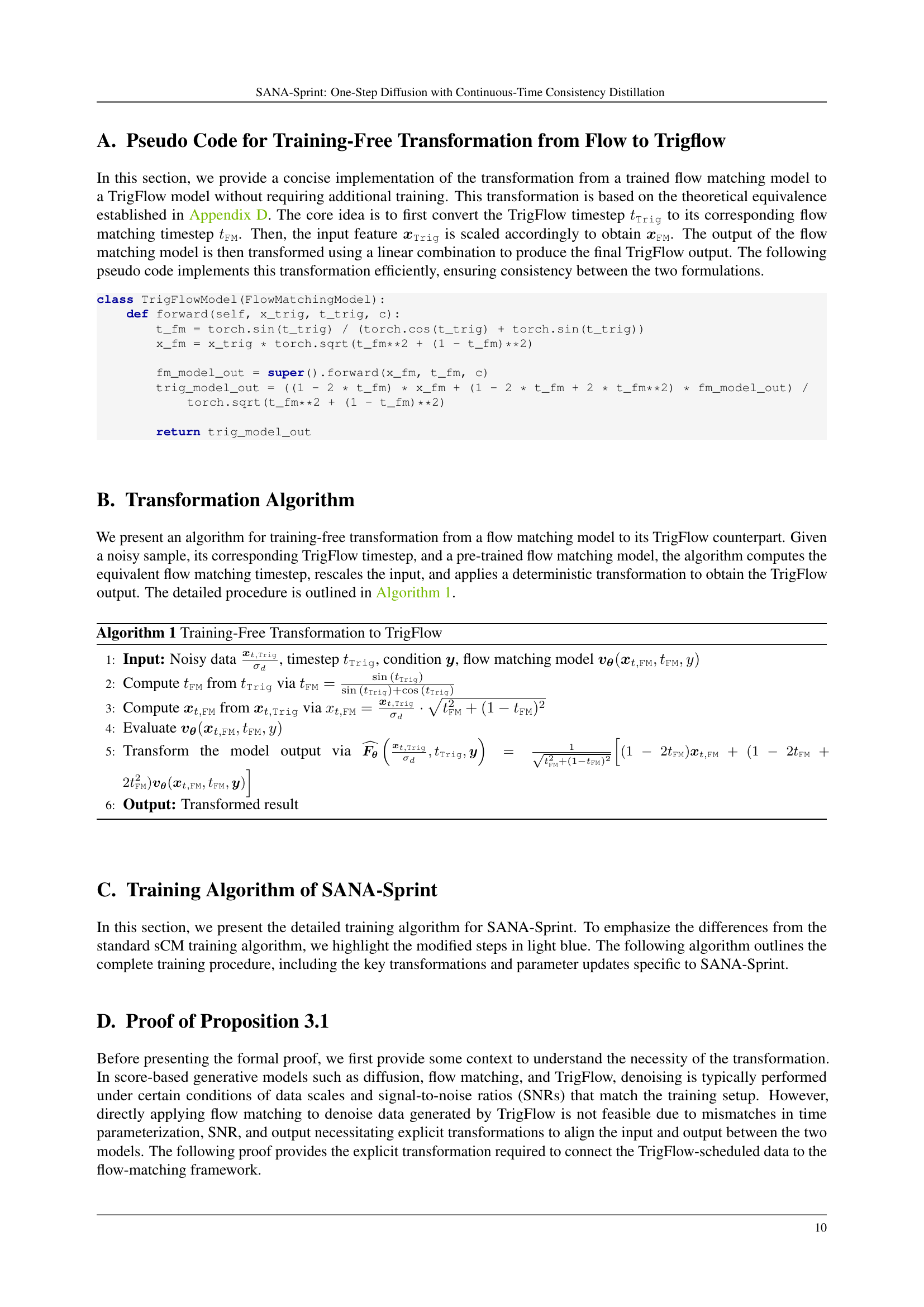
The paper introduces a novel training-free method to convert existing flow-matching models into TrigFlow models by employing mathematical transformations. This approach eliminates the necessity for distinct algorithm designs and extensive hyperparameter adjustments. SNR, timescale, and output are the key parameters in which the input and output must follow. This method facilitates the seamless incorporation of the continuous-time consistency model (sCM) framework with minimal adjustments. By adapting a lossless approach which follows a training algorithm which eliminates the need for a seperate trigflow model and still maintains performance.
sCM Stabilization#
While ‘sCM Stabilization’ isn’t a direct heading, the paper tackles stability issues in continuous-time consistency distillation (sCM). To mitigate these, they introduce a denser time embedding and integrate QK-Normalization into self- and cross-attention. The denser embedding likely provides a more nuanced representation of time, reducing ambiguity during distillation. QK-Normalization probably prevents gradient explosion, which can arise from scaling model sizes and increasing resolutions. These modifications facilitate efficient knowledge transfer and improve stability, enabling robust performance at higher resolutions and larger model sizes. In essence, the paper focuses on stabilizing the training process for sCM, allowing for more effective distillation and, ultimately, better image generation.
SANA-ControlNet#
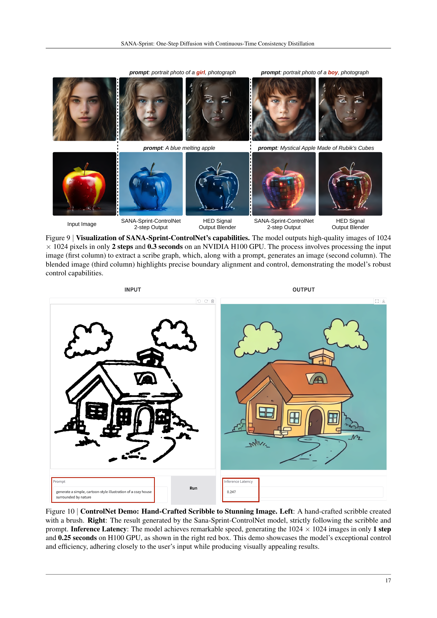
SANA-ControlNet appears to be an interesting fusion of the SANA architecture with ControlNet, aiming to enhance the controllability of image generation. This likely enables users to exert more precise control over the output by incorporating structural or spatial guidance. ControlNet’s ability to condition image generation on various inputs like edges or segmentation maps could be particularly powerful when combined with SANA’s efficient high-resolution synthesis. This combination potentially leads to a system where high-quality images can be generated with specific structural constraints in real-time, opening avenues for applications needing accurate content manipulation or creation based on user-defined layouts.
Max-Time Weighting#
Max-Time Weighting is a crucial strategy in diffusion models, especially for enhancing the one- and few-step generation capabilities, improving the generation quality. This technique likely involves prioritizing or emphasizing the later timesteps in the reverse diffusion process. By focusing on the max-time weighting, the model can better refine the image details and improve the overall quality, especially in the final stages of generation. It would be applied selectively, perhaps only during certain stages of training, to prevent overfitting and maintain the model’s generalization ability. It could involve dynamically adjusting the weights assigned to different timesteps during training, giving greater importance to those timesteps.
More visual insights#
More on figures

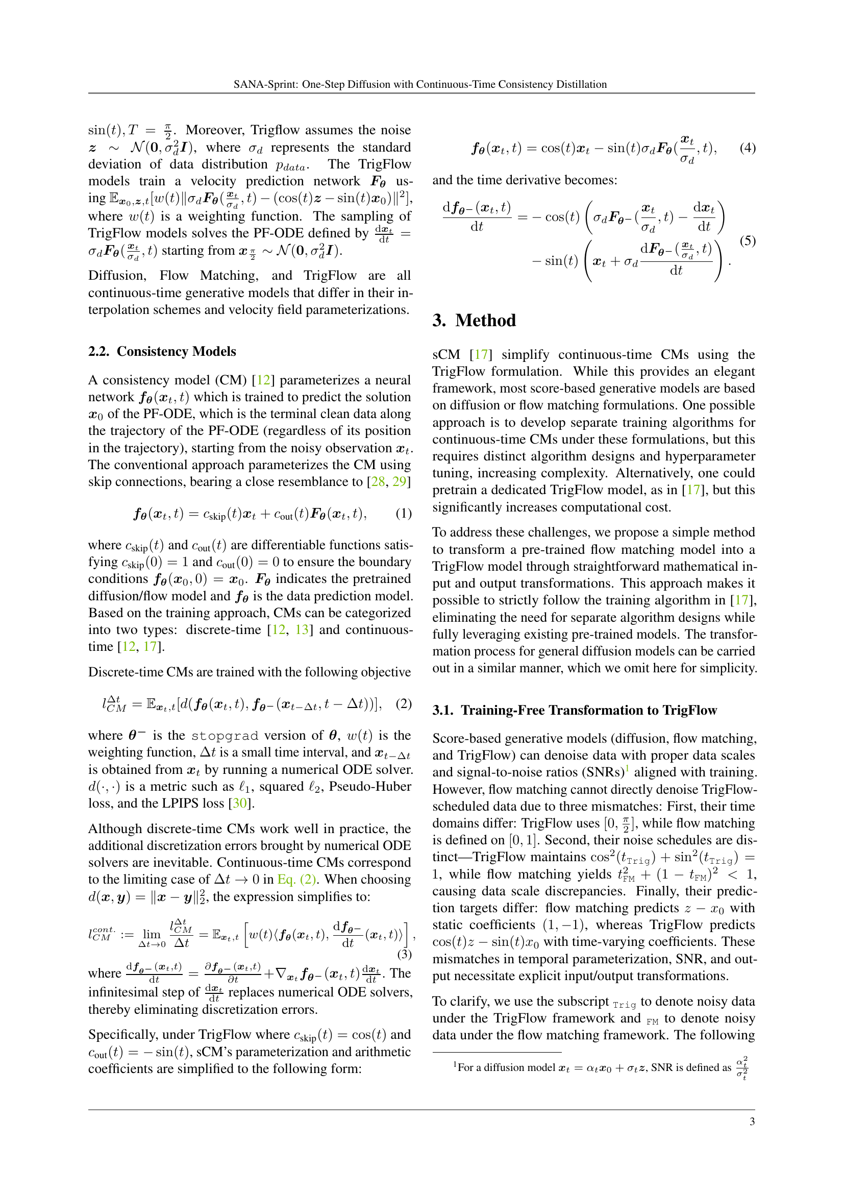
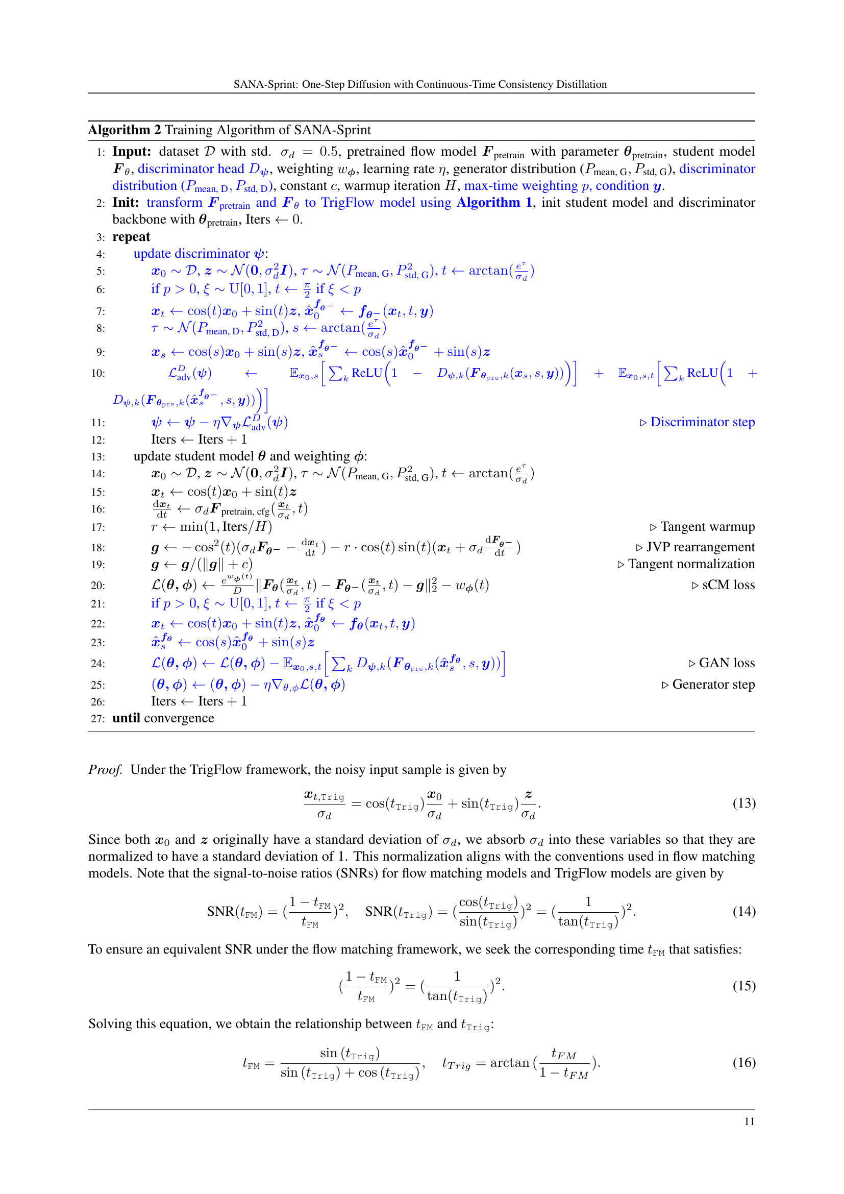
🔼 The figure illustrates the training process of the SANA-Sprint model. It uses a hybrid approach, combining continuous-time consistency model (sCM) training with Generative Adversarial Network (GAN) training. The student model is responsible for generating synthetic data and computing Jacobian-vector products (JVPs), while the teacher model provides velocity information (dx/dt) and features for the GAN loss function. This setup allows for simultaneous training of both sCM and GAN, simplifying the process and reducing computational overhead. Importantly, all training occurs solely in the latent space. Details regarding the training objective, the TrigFlow transformation (used to adapt a pre-trained model for sCM distillation), and specific equations are available in the paper’s Section 3.1 and Equations 9 and 11.
read the caption
Figure 2: Training paradigm of SANA-Sprint. In SANA-Sprint, we use the student model for synthetic data generation (x0^^subscript𝑥0\hat{x_{0}}over^ start_ARG italic_x start_POSTSUBSCRIPT 0 end_POSTSUBSCRIPT end_ARG) and JVP calculation, and we use the teacher model for velocity (dx/dtd𝑥d𝑡\mathrm{d}x/\mathrm{d}troman_d italic_x / roman_d italic_t) compute and its feature for the GAN loss, which allows us train sCM and GAN together and have only one training model purely in the latent space. Details of training objective and TrigFlow Transformation are in Eq. 9, Eq. 11 and Sec. 3.1.

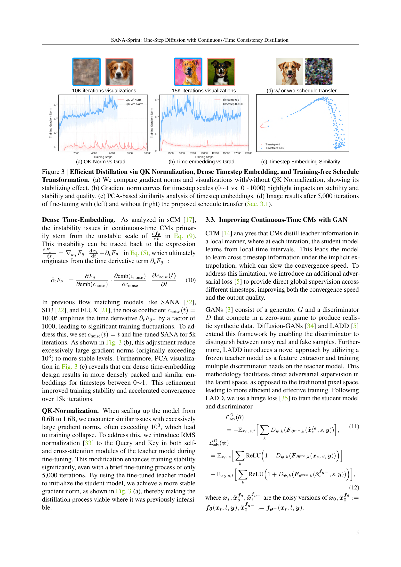
🔼 This figure demonstrates the effectiveness of three key improvements to the SANA-Sprint model’s training process: QK normalization, dense timestep embeddings, and training-free schedule transformation. Panel (a) shows a comparison of training gradient norms with and without QK normalization, illustrating the stabilizing impact. Panel (b) presents gradient norm curves comparing the use of two different timestep ranges (0-1 and 0-1000), highlighting how these impact stability and image quality. Panel (c) displays a PCA-based similarity analysis of the timestep embeddings, providing visual evidence of their relationships. Finally, Panel (d) displays image results after 5000 training iterations to showcase the effects of the proposed training-free schedule transformation, with images generated with (left) and without (right) this transformation.
read the caption
Figure 3: Efficient Distillation via QK Normalization, Dense Timestep Embedding, and Training-free Schedule Transformation. (a) We compare gradient norms and visualizations with/without QK Normalization, showing its stabilizing effect. (b) Gradient norm curves for timestep scales (0∼similar-to\sim∼1 vs. 0∼similar-to\sim∼1000) highlight impacts on stability and stability and quality. (c) PCA-based similarity analysis of timestep embeddings. (d) Image results after 5,000 iterations of fine-tuning with (left) and without (right) the proposed schedule transfer (Sec. 3.1).

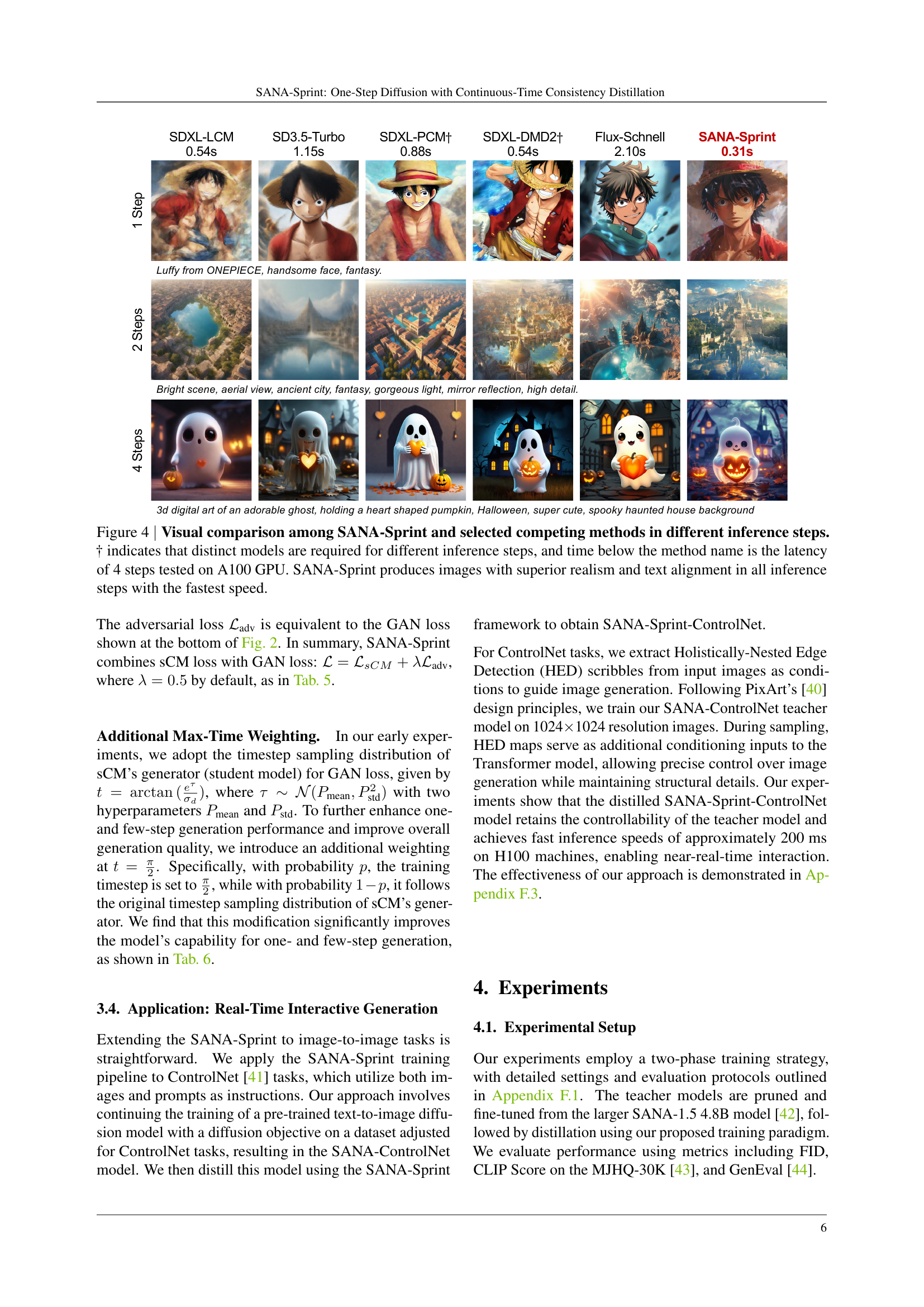
🔼 Figure 4 presents a comparison of image generation results from SANA-Sprint and other state-of-the-art diffusion models at varying numbers of inference steps (1, 2, and 4). The models are tested on the task of generating images from text prompts. The figure visually demonstrates the image quality generated by each method. It highlights that SANA-Sprint achieves superior realism and better text alignment compared to other methods across all inference step counts. Importantly, SANA-Sprint achieves this superior performance while also being significantly faster. The latency values shown beneath the method names represent the total inference time needed for 4 steps on an NVIDIA A100 GPU. The symbol † indicates that some models require separate training for each inference step count, unlike SANA-Sprint, which uses a single unified model across all step counts.
read the caption
Figure 4: Visual comparison among SANA-Sprint and selected competing methods in different inference steps. † indicates that distinct models are required for different inference steps, and time below the method name is the latency of 4 steps tested on A100 GPU. SANA-Sprint produces images with superior realism and text alignment in all inference steps with the fastest speed.

🔼 This table presents the results of an ablation study comparing different loss function combinations used in training the SANA-Sprint model. It shows how combining the continuous-time consistency model (sCM) loss with the latent adversarial distillation (LADD) loss affects the model’s performance, as measured by FID and CLIP scores. The table allows researchers to understand the individual contributions of each loss component and their optimal balance for effective training.
read the caption
Table 3: Comparison of loss combination.

🔼 This table presents a comparison of different Classifier-Free Guidance (CFG) training strategies used in the SANA-Sprint model. It shows how the choice of CFG embedding strategy (with or without embedding) affects the final model’s performance, as measured by FID (Fréchet Inception Distance) and CLIP score (a measure of text-image alignment). This helps to understand the impact of different training approaches on the model’s ability to generate images that accurately reflect the user’s textual prompts.
read the caption
Table 4: Comparison of CFG training strategies.

🔼 This table presents an ablation study comparing different weightings of the continuous-time consistency model (sCM) loss and the latent adversarial distillation (LADD) loss. It shows how varying the balance between these two loss functions affects the final model performance, measured by FID and CLIP scores.
read the caption
Table 5: sCM and LADD loss weighting.

🔼 This table presents an ablation study on the effect of different max-time weighting strategies on the performance of the SANA-Sprint model. The max-time weighting strategy modifies the training process by randomly selecting a timestep at the maximum value (t = π/2) with a certain probability, while the rest of the timesteps are sampled according to the model’s original distribution. The table compares the FID and CLIP scores achieved with different max-time probabilities (0%, 50%, 70%), showing how this approach impacts the overall quality of the generated images.
read the caption
Table 6: Comparison of max-time weighting strategy.

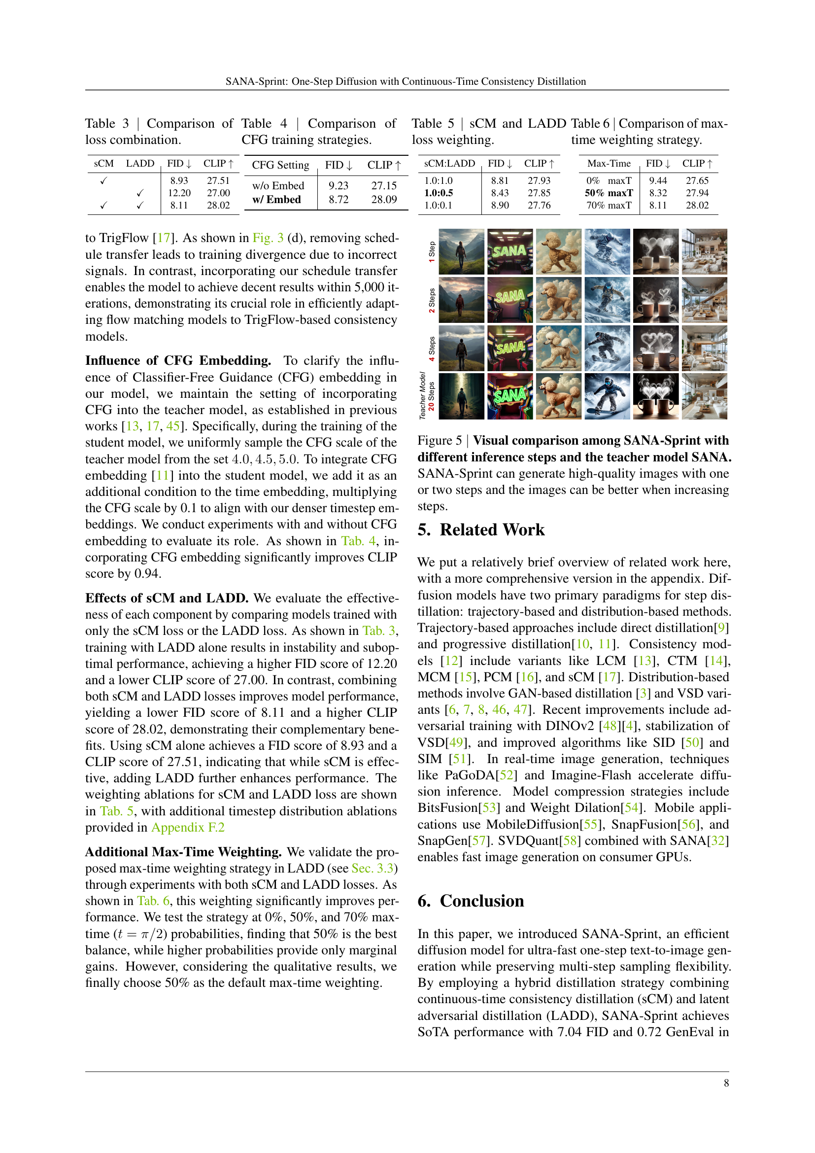
🔼 This figure compares image generation results of SANA-Sprint with varying numbers of inference steps (1, 2, and 4) against its 20-step teacher model, SANA. It visually demonstrates that SANA-Sprint can produce high-quality images even with a significantly reduced number of steps, showcasing the effectiveness of the proposed one-step diffusion method. The improvement in image quality is noticeable as the number of steps increases from one to four, while still maintaining superior speed compared to the teacher model.
read the caption
Figure 5: Visual comparison among SANA-Sprint with different inference steps and the teacher model SANA. SANA-Sprint can generate high-quality images with one or two steps and the images can be better when increasing steps.

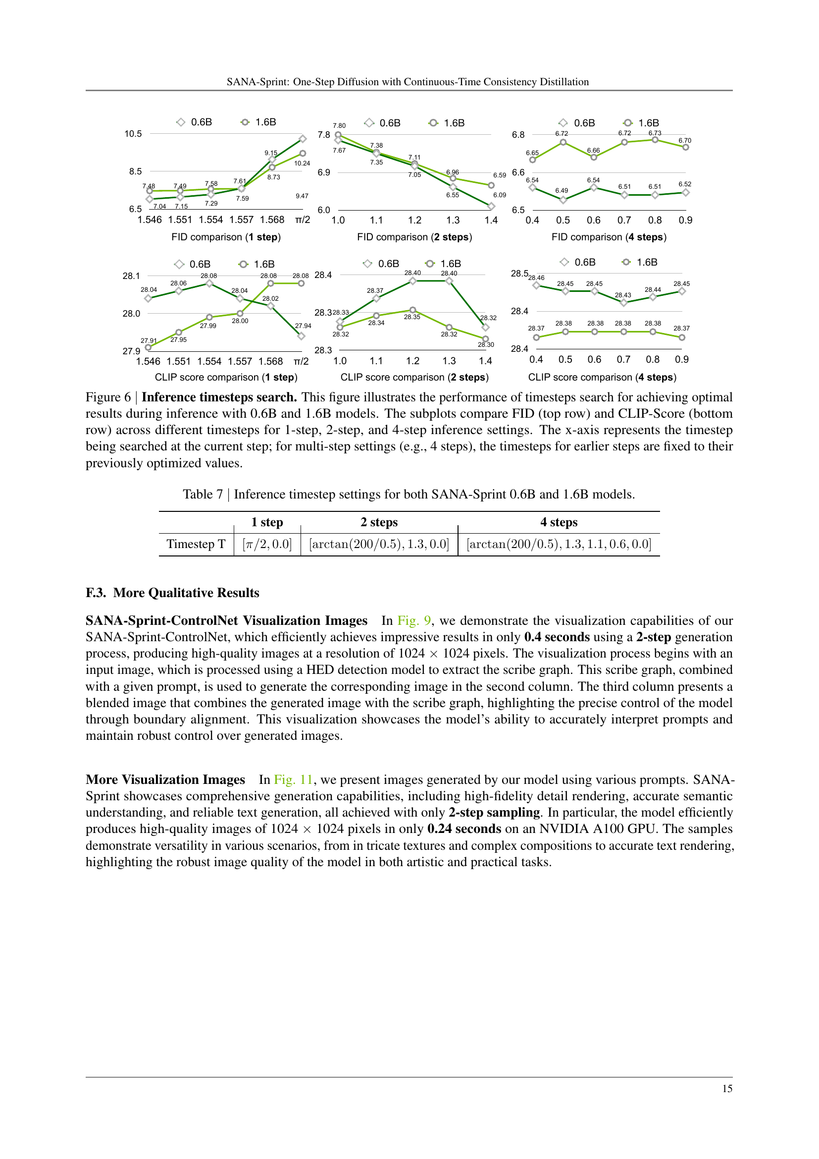
🔼 This figure visualizes the process of finding the optimal timestep settings for inference with SANA-Sprint models of sizes 0.6B and 1.6B parameters. It explores the impact of timestep choices on the FID (Frechet Inception Distance) and CLIP (Contrastive Language-Image Pre-training) scores for different inference scenarios (1-step, 2-step, and 4-step). Each subplot displays the FID and CLIP scores obtained for various timesteps. For multi-step inference, previously optimized timesteps from earlier steps are retained, making the search more efficient and focused.
read the caption
Figure 6: Inference timesteps search. This figure illustrates the performance of timesteps search for achieving optimal results during inference with 0.6B and 1.6B models. The subplots compare FID (top row) and CLIP-Score (bottom row) across different timesteps for 1-step, 2-step, and 4-step inference settings. The x-axis represents the timestep being searched at the current step; for multi-step settings (e.g., 4 steps), the timesteps for earlier steps are fixed to their previously optimized values.

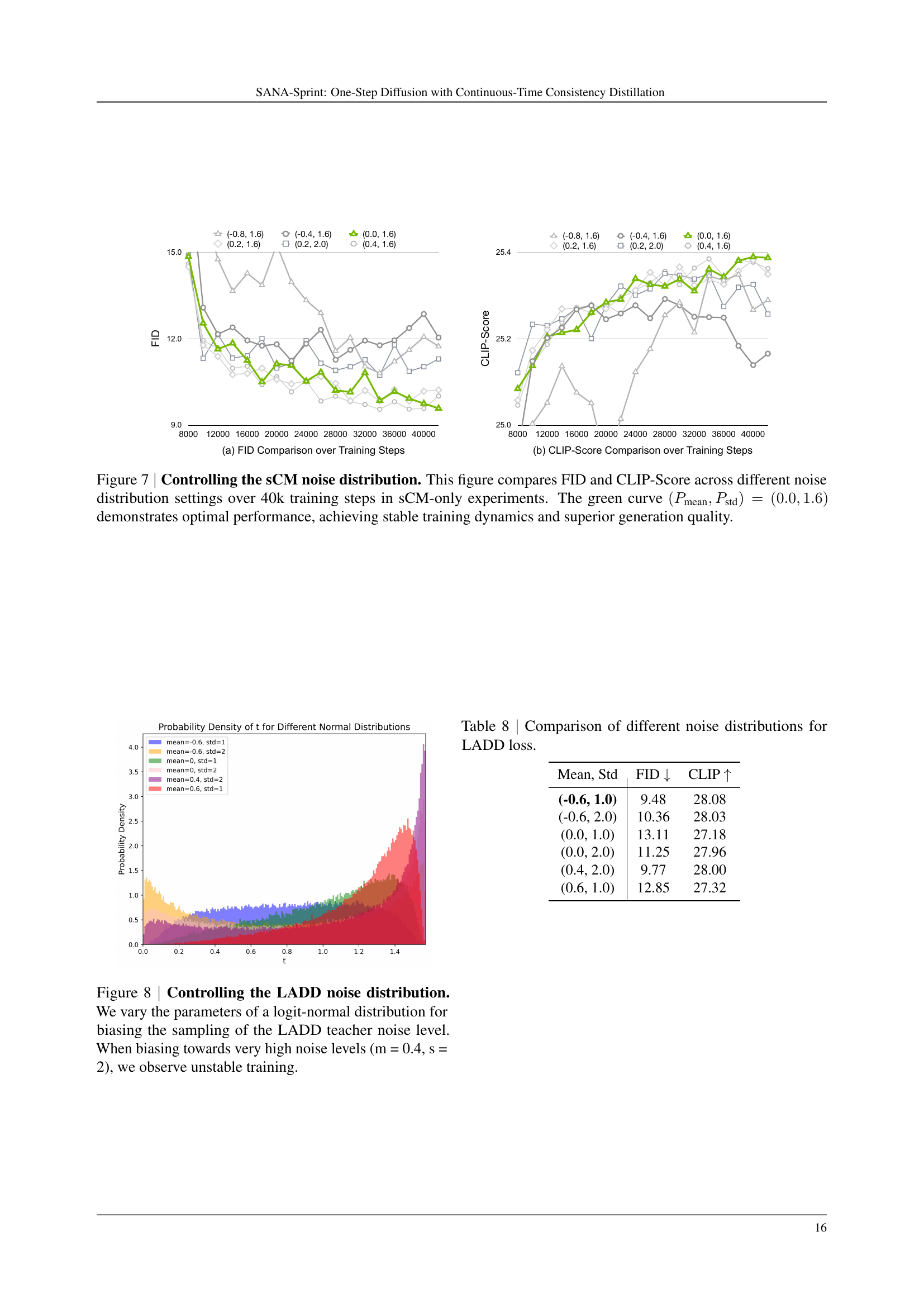
🔼 The figure displays the impact of various noise distribution configurations on the performance of the continuous-time consistency model (sCM) during training. The x-axis represents the training steps (up to 40,000), and the y-axis shows the FID (Fréchet Inception Distance) and CLIP (Contrastive Language-Image Pre-training) scores, which are used to evaluate image quality and similarity to text prompts respectively. Multiple lines depict the results for different configurations of the mean (Pmean) and standard deviation (Pstd) of the noise distribution. The plot reveals that the configuration with Pmean=0.0 and Pstd=1.6 (green line) yields the best results, achieving both low FID (indicating high-quality images) and high CLIP scores (showing good alignment with text prompts) while maintaining stable training dynamics. Other configurations exhibit either instability during training or suboptimal performance.
read the caption
Figure 7: Controlling the sCM noise distribution. This figure compares FID and CLIP-Score across different noise distribution settings over 40k training steps in sCM-only experiments. The green curve (Pmean,Pstd)=(0.0,1.6)subscript𝑃meansubscript𝑃std0.01.6(P_{\text{mean}},P_{\text{std}})=(0.0,1.6)( italic_P start_POSTSUBSCRIPT mean end_POSTSUBSCRIPT , italic_P start_POSTSUBSCRIPT std end_POSTSUBSCRIPT ) = ( 0.0 , 1.6 ) demonstrates optimal performance, achieving stable training dynamics and superior generation quality.
More on tables
| Methods | Inference | Throughput | Latency | Params | FID | CLIP | GenEval | |
| steps | (samples/s) | (s) | (B) | |||||
| Pre-train Models | SDXL [36] | 50 | 0.15 | 6.5 | 2.6 | 6.63 | 29.03 | 0.55 |
| PixArt- [37] | 20 | 0.4 | 2.7 | 0.6 | 6.15 | 28.26 | 0.54 | |
| SD3-medium [38] | 28 | 0.28 | 4.4 | 2.0 | 11.92 | 27.83 | 0.62 | |
| FLUX-dev [21] | 50 | 0.04 | 23.0 | 12.0 | 10.15 | 27.47 | 0.67 | |
| Playground v3 [39] | - | 0.06 | 15.0 | 24 | - | - | 0.76 | |
| SANA 0.6B [32] | 20 | 1.7 | 0.9 | 0.6 | 5.81 | 28.36 | 0.64 | |
| SANA 1.6B [32] | 20 | 1.0 | 1.2 | 1.6 | 5.76 | 28.67 | 0.66 | |
| Distillation Models | SDXL-LCM [13] | 4 | 2.27 | 0.54 | 0.9 | 10.81 | 28.10 | 0.53 |
| PixArt-LCM [40] | 4 | 2.61 | 0.50 | 0.6 | 8.63 | 27.40 | 0.44 | |
| PCM [16]† | 4 | 1.95 | 0.88 | 0.9 | 15.55 | 27.53 | 0.56 | |
| SD3.5-Turbo [22] | 4 | 0.94 | 1.15 | 8.0 | 11.97 | 27.35 | 0.72 | |
| SDXL-DMD2 [20]† | 4 | 2.27 | 0.54 | 0.9 | 6.82 | 28.84 | 0.60 | |
| FLUX-schnell [21] | 4 | 0.5 | 2.10 | 12.0 | 7.94 | 28.14 | 0.71 | |
| SANA-Sprint 0.6B | 4 | 5.34 | 0.32 | 0.6 | 6.48 | 28.45 | 0.76 | |
| SANA-Sprint 1.6B | 4 | 5.20 | 0.31 | 1.6 | 6.66 | 28.38 | 0.77 | |
| SDXL-LCM [13] | 2 | 2.89 | 0.40 | 0.9 | 18.11 | 27.51 | 0.44 | |
| PixArt-LCM [40] | 2 | 3.52 | 0.31 | 0.6 | 10.33 | 27.24 | 0.42 | |
| SD3.5-Turbo [22] | 2 | 1.61 | 0.68 | 8.0 | 51.47 | 25.59 | 0.53 | |
| PCM [16]† | 2 | 2.62 | 0.56 | 0.9 | 14.70 | 27.66 | 0.55 | |
| SDXL-DMD2 [20]† | 2 | 2.89 | 0.40 | 0.9 | 7.61 | 28.87 | 0.58 | |
| FLUX-schnell [21] | 2 | 0.92 | 1.15 | 12.0 | 7.75 | 28.25 | 0.71 | |
| SANA-Sprint 0.6B | 2 | 6.46 | 0.25 | 0.6 | 6.54 | 28.40 | 0.76 | |
| SANA-Sprint 1.6B | 2 | 5.68 | 0.24 | 1.6 | 6.76 | 28.32 | 0.77 | |
| SDXL-LCM [13] | 1 | 3.36 | 0.32 | 0.9 | 50.51 | 24.45 | 0.28 | |
| PixArt-LCM [40] | 1 | 4.26 | 0.25 | 0.6 | 73.35 | 23.99 | 0.41 | |
| PixArt-DMD [37]† | 1 | 4.26 | 0.25 | 0.6 | 9.59 | 26.98 | 0.45 | |
| SD3.5-Turbo [22] | 1 | 2.48 | 0.45 | 8.0 | 52.40 | 25.40 | 0.51 | |
| PCM [16]† | 1 | 3.16 | 0.40 | 0.9 | 30.11 | 26.47 | 0.42 | |
| SDXL-DMD2 [20]† | 1 | 3.36 | 0.32 | 0.9 | 7.10 | 28.93 | 0.59 | |
| FLUX-schnell [21] | 1 | 1.58 | 0.68 | 12.0 | 7.26 | 28.49 | 0.69 | |
| SANA-Sprint 0.6B | 1 | 7.22 | 0.21 | 0.6 | 7.04 | 28.04 | 0.72 | |
| SANA-Sprint 1.6B | 1 | 6.71 | 0.21 | 1.6 | 7.59 | 28.00 | 0.74 | |
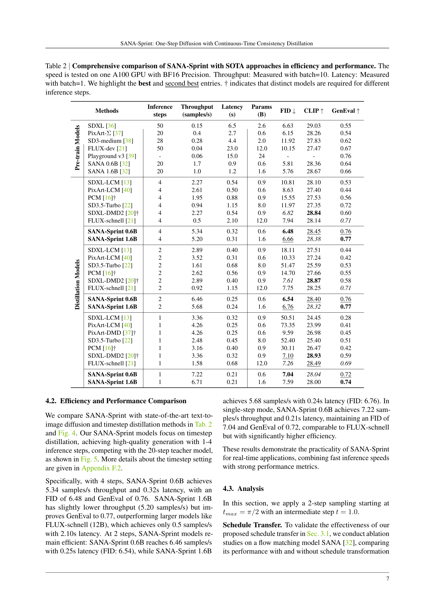
🔼 Table 2 presents a comprehensive comparison of SANA-Sprint’s performance and efficiency against state-of-the-art (SOTA) approaches in text-to-image generation. The results are measured using various metrics including FID (Fréchet Inception Distance), CLIP (Contrastive Language-Image Pre-training) score, and GenEval score. These metrics evaluate image quality, alignment between generated images and text prompts, and overall generation quality. The table also provides information on the inference speed measured in samples per second (throughput) and latency in seconds, tested on a single NVIDIA A100 GPU using BF16 precision. The throughput is measured with a batch size of 10, and latency is measured with a batch size of 1. The best and second-best results are highlighted for each metric. Note that the † symbol indicates models where different architectures were required for different numbers of inference steps.
read the caption
Table 2: Comprehensive comparison of SANA-Sprint with SOTA approaches in efficiency and performance. The speed is tested on one A100 GPU with BF16 Precision. Throughput: Measured with batch=10. Latency: Measured with batch=1. We highlight the best and second best entries. † indicates that distinct models are required for different inference steps.
| sCM | LADD | FID | CLIP |
| ✓ | 8.93 | 27.51 | |
| ✓ | 12.20 | 27.00 | |
| ✓ | ✓ | 8.11 | 28.02 |
🔼 This table details the optimal timestep settings used for inference in the SANA-Sprint model, categorized by the number of inference steps (1, 2, or 4) and the model size (0.6B or 1.6B parameters). Each setting represents the specific timesteps used during the denoising process to generate images efficiently and with high quality. The settings were obtained through an optimization process, as explained in the paper, to find the most effective timesteps for each combination of steps and model size.
read the caption
Table 7: Inference timestep settings for both SANA-Sprint 0.6B and 1.6B models.
| CFG Setting | FID | CLIP |
| w/o Embed | 9.23 | 27.15 |
| w/ Embed | 8.72 | 28.09 |
🔼 This table presents a comparison of different noise distribution configurations used within the Latent Adversarial Diffusion Distillation (LADD) loss function. The experiment aims to find the optimal configuration that balances training stability and generation quality. The comparison is done by varying the mean and standard deviation parameters of the noise distribution and observing the resulting FID and CLIP scores. The results showcase how different noise distributions affect model performance.
read the caption
Table 8: Comparison of different noise distributions for LADD loss.
Full paper#