TL;DR#
Autoregressive (AR) models have excelled, especially in language modeling. However, applying next-token prediction to image generation presents challenges since images are structured in a 2D space. Standard AR models struggle with tasks like inpainting and outpainting because generation follows a specific token order, especially in high-resolution. Furthermore, using bidirectional attention, as in MaskGIT, prevents the use of the KV cache, increasing overhead. Thus, there is a need for a framework to support flexible generation orders and maintain efficiency.
This paper introduces a visual Autoregressive model, ARPG, enabling Randomized Parallel Generation. It uses a novel ‘guided decoding’ that decouples positional guidance from content representation. This enables random-order training and generation without needing bidirectional attention. ARPG supports parallel inference by concurrently processing multiple queries using a shared KV cache. It achieves state-of-the-art results in image generation, improving throughput and reducing memory usage compared to existing autoregressive models.
Key Takeaways#
Why does it matter?#
This paper introduces a novel AR framework for image generation, offering a pathway to improve model efficiency and quality while simultaneously reducing memory consumption. This research aligns with the growing interest in efficient and scalable autoregressive models.
Visual Insights#

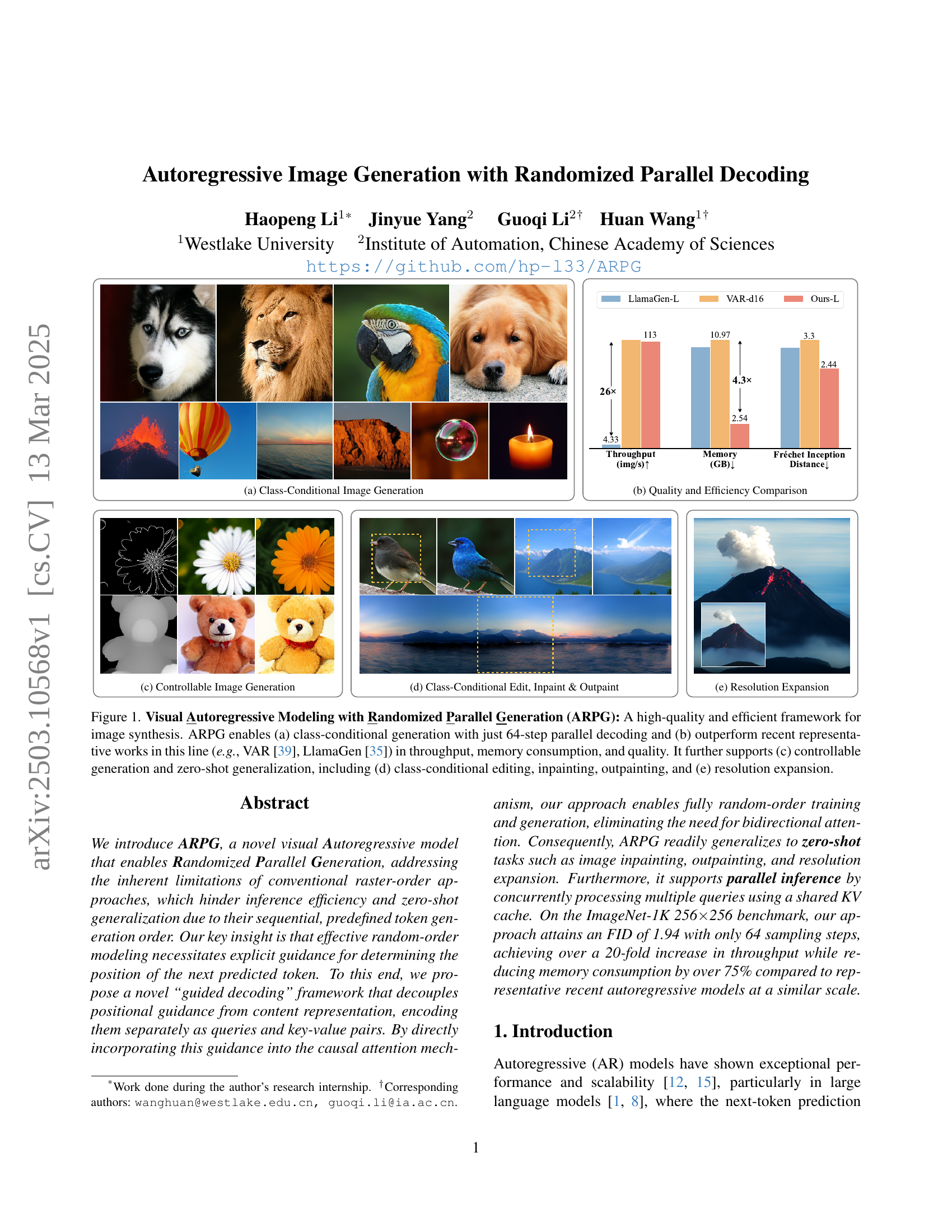
🔼 This figure showcases the capabilities of the ARPG model for autoregressive image generation. Panel (a) demonstrates class-conditional image generation, achieving high quality with only 64 parallel decoding steps. Panel (b) presents a quantitative comparison, highlighting ARPG’s superior performance over state-of-the-art methods (VAR and LlamaGen) in terms of speed (throughput), memory efficiency, and image quality (FID). The remaining panels illustrate the model’s versatility: (c) controllable generation, (d) zero-shot capabilities (editing, inpainting, and outpainting), and (e) resolution expansion.
read the caption
Figure 1: Visual Autoregressive Modeling with Randomized Parallel Generation (ARPG): A high-quality and efficient framework for image synthesis. ARPG enables (a) class-conditional generation with just 64-step parallel decoding and (b) outperform recent representative works in this line (e.g., VAR [39], LlamaGen [35]) in throughput, memory consumption, and quality. It further supports (c) controllable generation and zero-shot generalization, including (d) class-conditional editing, inpainting, outpainting, and (e) resolution expansion.
| Model | Layers | Hidden Size | Heads | Parameters |
|---|---|---|---|---|
| ARPG-L | 12+12 | 1024 | 16 | 320 M |
| ARPG-XL | 18+18 | 1280 | 20 | 719 M |
| ARPG-XXL | 24+24 | 1536 | 24 | 1.3 B |
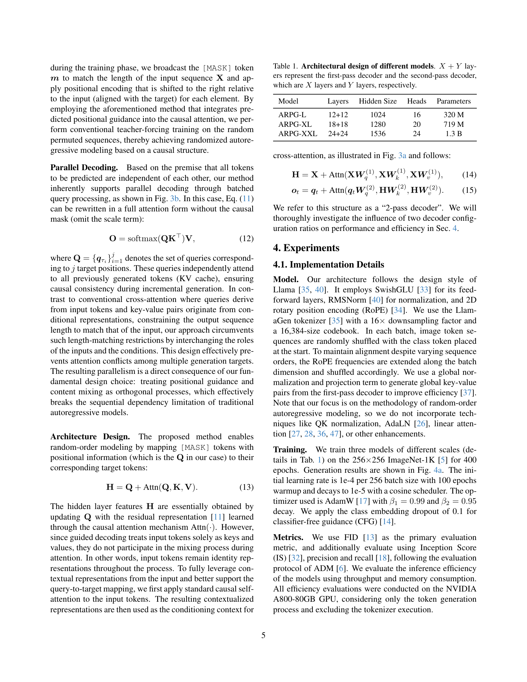
🔼 This table details the architecture of three different autoregressive models (ARPG-L, ARPG-XL, and ARPG-XXL). It shows the number of layers in the first-pass decoder and second-pass decoder, the hidden size, the number of attention heads, and the total number of parameters for each model. The first-pass decoder extracts contextual representations, while the second-pass decoder utilizes target-aware queries to guide the prediction process. The table highlights the scalability of the ARPG model architecture as the model size increases.
read the caption
Table 1: Architectural design of different models. X+Y𝑋𝑌X+Yitalic_X + italic_Y layers represent the first-pass decoder and the second-pass decoder, which are X𝑋Xitalic_X layers and Y𝑌Yitalic_Y layers, respectively.
In-depth insights#
Guided Decoding#
Guided decoding suggests a targeted approach to autoregressive generation, moving beyond the traditional raster-scan order. The core idea revolves around explicitly guiding the generation process to determine the next token’s position. This is achieved by decoupling positional guidance from content representation, which is encoded as queries and key-value pairs, and incorporating the guidance directly into the causal attention mechanism. By doing this it ensures that random-order training and generation are possible, eliminating the necessity for bidirectional attention. The benefits are zero-shot generalization capabilities, which enable more efficient parallel decoding by processing multiple queries simultaneously with shared KV cache. In essence, guided decoding represents a significant departure from standard autoregressive techniques, offering a more efficient and flexible approach to generative modeling.
Parallelization#
Parallelization is crucial for efficient image generation. Traditional autoregressive models are sequential, limiting speed. This research likely introduces a method to break this dependency, allowing simultaneous processing of different image regions or tokens. Shared KV cache enables parallel decoding of all tokens to be predicted, it can significantly boost throughput without excessive memory. By processing multiple queries simultaneously, the framework likely achieves substantial speedups compared to standard autoregressive approaches. The method probably leverages techniques that breaks the image into independent segments. The key is probably efficient management of dependencies and a robust parallel processing strategy.
Zero-Shot AR#
Zero-shot autoregressive (AR) models represent a fascinating frontier in generative modeling, exhibiting the capacity to produce outputs for unseen tasks without explicit retraining. This capability stems from the model’s ability to learn a generalizable representation of the underlying data distribution. A key challenge lies in designing architectures and training strategies that promote this generalization. Techniques such as meta-learning, auxiliary tasks, and contrastive learning can be employed to enhance the model’s adaptability. Furthermore, careful consideration must be given to the model’s inductive biases to ensure that it is well-suited to the target domain. Evaluation of zero-shot AR models requires the use of appropriate metrics that can assess the quality and diversity of the generated outputs, as well as their relevance to the unseen tasks. Analyzing failure cases is also crucial for identifying areas where the model can be improved. As the field of AR modeling continues to evolve, zero-shot learning promises to unlock new possibilities for creative and intelligent systems.
2-Pass Decoder#
The concept of a ‘2-Pass Decoder,’ while not explicitly detailed, suggests a strategy to refine autoregressive image generation. It likely involves an initial pass to capture global context and create key-value pairs representing this distilled information. A subsequent pass would then use target-aware queries to selectively attend to this global context, guiding the generation of individual tokens. This approach could balance computational efficiency, by processing the entire image initially, with precise, localized control during token generation. The potential benefits include better handling of long-range dependencies and improved coherence in the generated image, all while leveraging parallel processing for speed. Further investigation into how these passes are structured, what information is carried, and how the attention mechanisms operate would be needed to fully understand its impact.
Token Ordering#
The token ordering in autoregressive image generation is a critical factor influencing both efficiency and quality. Traditional raster-scan orders limit parallelization and generalization to tasks requiring non-causal dependencies like inpainting. Randomized token orders offer flexibility, potentially improving zero-shot capabilities. However, effective random ordering necessitates explicit positional guidance to avoid prediction ambiguity. Methods like positional instruction tokens incur overhead, highlighting the challenge of balancing flexibility with computational cost. The design of the token ordering strategy directly impacts the model’s ability to capture long-range dependencies and generate coherent images, demanding a careful consideration of trade-offs.
More visual insights#
More on figures

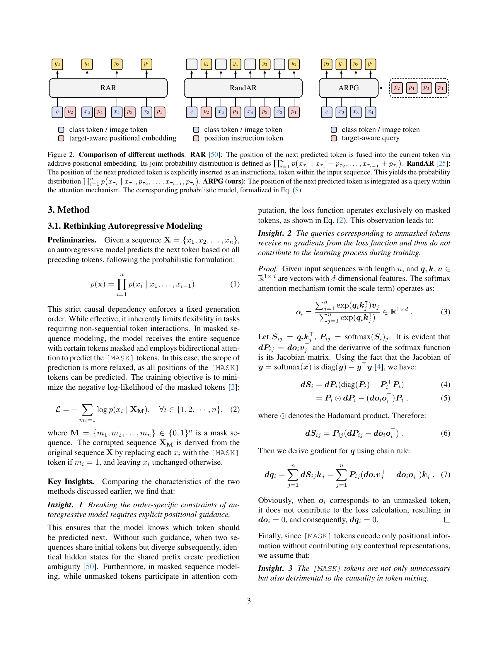
🔼 Figure 2 illustrates the differences in how three different autoregressive models (RAR, RandAR, and ARPG) handle the positional information of the next predicted token during image generation. RAR fuses positional information into the current token using additive positional embedding. RandAR explicitly inserts the position as an instructional token in the input sequence. ARPG integrates positional information into the query of the attention mechanism, decoupling positional guidance from content representation. The corresponding probability models for RAR and RandAR are shown, highlighting their differences in incorporating position information.
read the caption
Figure 2: Comparison of different methods. RAR [50]: The position of the next predicted token is fused into the current token via additive positional embedding. Its joint probability distribution is defined as ∏i=1np(xτi∣xτ1+pτ2,…,xτi−1+pτi)superscriptsubscriptproduct𝑖1𝑛𝑝conditionalsubscript𝑥subscript𝜏𝑖subscript𝑥subscript𝜏1subscript𝑝subscript𝜏2…subscript𝑥subscript𝜏𝑖1subscript𝑝subscript𝜏𝑖\prod_{i=1}^{n}p\big{(}x_{\tau_{i}}\mid x_{\tau_{1}}+p_{\tau_{2}},\dots,x_{% \tau_{i-1}}+p_{\tau_{i}}\big{)}∏ start_POSTSUBSCRIPT italic_i = 1 end_POSTSUBSCRIPT start_POSTSUPERSCRIPT italic_n end_POSTSUPERSCRIPT italic_p ( italic_x start_POSTSUBSCRIPT italic_τ start_POSTSUBSCRIPT italic_i end_POSTSUBSCRIPT end_POSTSUBSCRIPT ∣ italic_x start_POSTSUBSCRIPT italic_τ start_POSTSUBSCRIPT 1 end_POSTSUBSCRIPT end_POSTSUBSCRIPT + italic_p start_POSTSUBSCRIPT italic_τ start_POSTSUBSCRIPT 2 end_POSTSUBSCRIPT end_POSTSUBSCRIPT , … , italic_x start_POSTSUBSCRIPT italic_τ start_POSTSUBSCRIPT italic_i - 1 end_POSTSUBSCRIPT end_POSTSUBSCRIPT + italic_p start_POSTSUBSCRIPT italic_τ start_POSTSUBSCRIPT italic_i end_POSTSUBSCRIPT end_POSTSUBSCRIPT ). RandAR [25]: The position of the next predicted token is explicitly inserted as an instructional token within the input sequence. This yields the probability distribution ∏i=1np(xτi∣xτ1,pτ2,…,xτi−1,pτi)superscriptsubscriptproduct𝑖1𝑛𝑝conditionalsubscript𝑥subscript𝜏𝑖subscript𝑥subscript𝜏1subscript𝑝subscript𝜏2…subscript𝑥subscript𝜏𝑖1subscript𝑝subscript𝜏𝑖\prod_{i=1}^{n}p\big{(}x_{\tau_{i}}\mid x_{\tau_{1}},p_{\tau_{2}},\dots,x_{% \tau_{i-1}},p_{\tau_{i}}\big{)}∏ start_POSTSUBSCRIPT italic_i = 1 end_POSTSUBSCRIPT start_POSTSUPERSCRIPT italic_n end_POSTSUPERSCRIPT italic_p ( italic_x start_POSTSUBSCRIPT italic_τ start_POSTSUBSCRIPT italic_i end_POSTSUBSCRIPT end_POSTSUBSCRIPT ∣ italic_x start_POSTSUBSCRIPT italic_τ start_POSTSUBSCRIPT 1 end_POSTSUBSCRIPT end_POSTSUBSCRIPT , italic_p start_POSTSUBSCRIPT italic_τ start_POSTSUBSCRIPT 2 end_POSTSUBSCRIPT end_POSTSUBSCRIPT , … , italic_x start_POSTSUBSCRIPT italic_τ start_POSTSUBSCRIPT italic_i - 1 end_POSTSUBSCRIPT end_POSTSUBSCRIPT , italic_p start_POSTSUBSCRIPT italic_τ start_POSTSUBSCRIPT italic_i end_POSTSUBSCRIPT end_POSTSUBSCRIPT ). ARPG (ours): The position of the next predicted token is integrated as a query within the attention mechanism. The corresponding probabilistic model, formalized in Eq. (8).

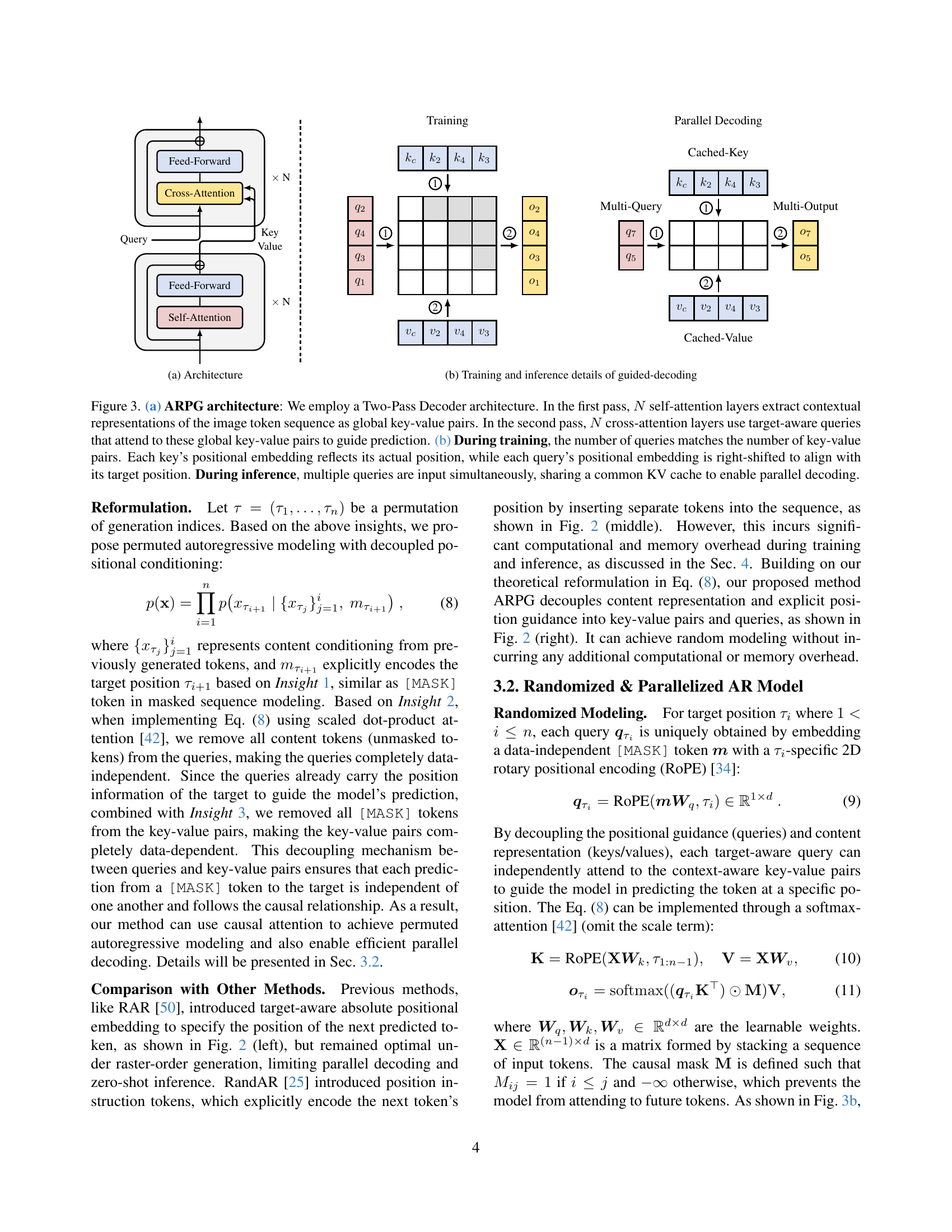
🔼 This figure shows the architecture of the ARPG model, a two-pass decoder architecture. The first pass uses self-attention layers to extract contextual representations of image tokens as key-value pairs. The second pass uses cross-attention layers with target-aware queries that attend to these key-value pairs to guide the prediction. During training, the number of queries matches the number of key-value pairs. The positional embedding of each key reflects its actual position, while the positional embedding of each query is shifted right to align with its target position. During inference, multiple queries are input simultaneously, sharing a common KV cache to enable parallel decoding. This architecture enables training and inference in fully random token order.
read the caption
(a) Architecture

🔼 This figure illustrates the training and inference mechanisms of the guided decoding process in ARPG. During training, the number of queries matches the number of key-value pairs. Each query’s positional embedding is right-shifted to align with its target position, while each key’s positional embedding reflects its actual position. This allows the model to learn to predict tokens at random positions. During inference, however, multiple queries are input concurrently, sharing a common KV cache to enable parallel decoding. This shared cache drastically improves efficiency.
read the caption
(b) Training and inference details of guided-decoding

🔼 Figure 3 illustrates the ARPG architecture, a two-pass decoder model. The first pass uses self-attention layers to process the image token sequence and generate global key-value pairs representing contextual information. The second pass employs cross-attention layers with ’target-aware queries’ to focus on specific parts of the global key-value pairs, guiding the prediction process. During training, the number of queries equals the number of key-value pairs. Each key’s positional embedding indicates its position in the sequence, while each query’s embedding is offset to point to the position of the token to be predicted. This design allows for parallel decoding during inference because multiple queries can be processed simultaneously using a shared key-value cache.
read the caption
Figure 3: 3(a) ARPG architecture: We employ a Two-Pass Decoder architecture. In the first pass, N𝑁Nitalic_N self-attention layers extract contextual representations of the image token sequence as global key-value pairs. In the second pass, N𝑁Nitalic_N cross-attention layers use target-aware queries that attend to these global key-value pairs to guide prediction. 3(b) During training, the number of queries matches the number of key-value pairs. Each key’s positional embedding reflects its actual position, while each query’s positional embedding is right-shifted to align with its target position. During inference, multiple queries are input simultaneously, sharing a common KV cache to enable parallel decoding.

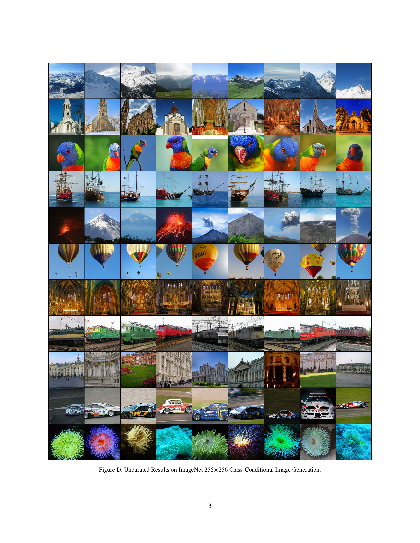
🔼 This figure shows several images generated by the ARPG model given different class labels. It demonstrates the model’s ability to generate high-quality, diverse images conditioned on class information. Each image in the grid represents a different class.
read the caption
(a) Class-Conditional Image Generation

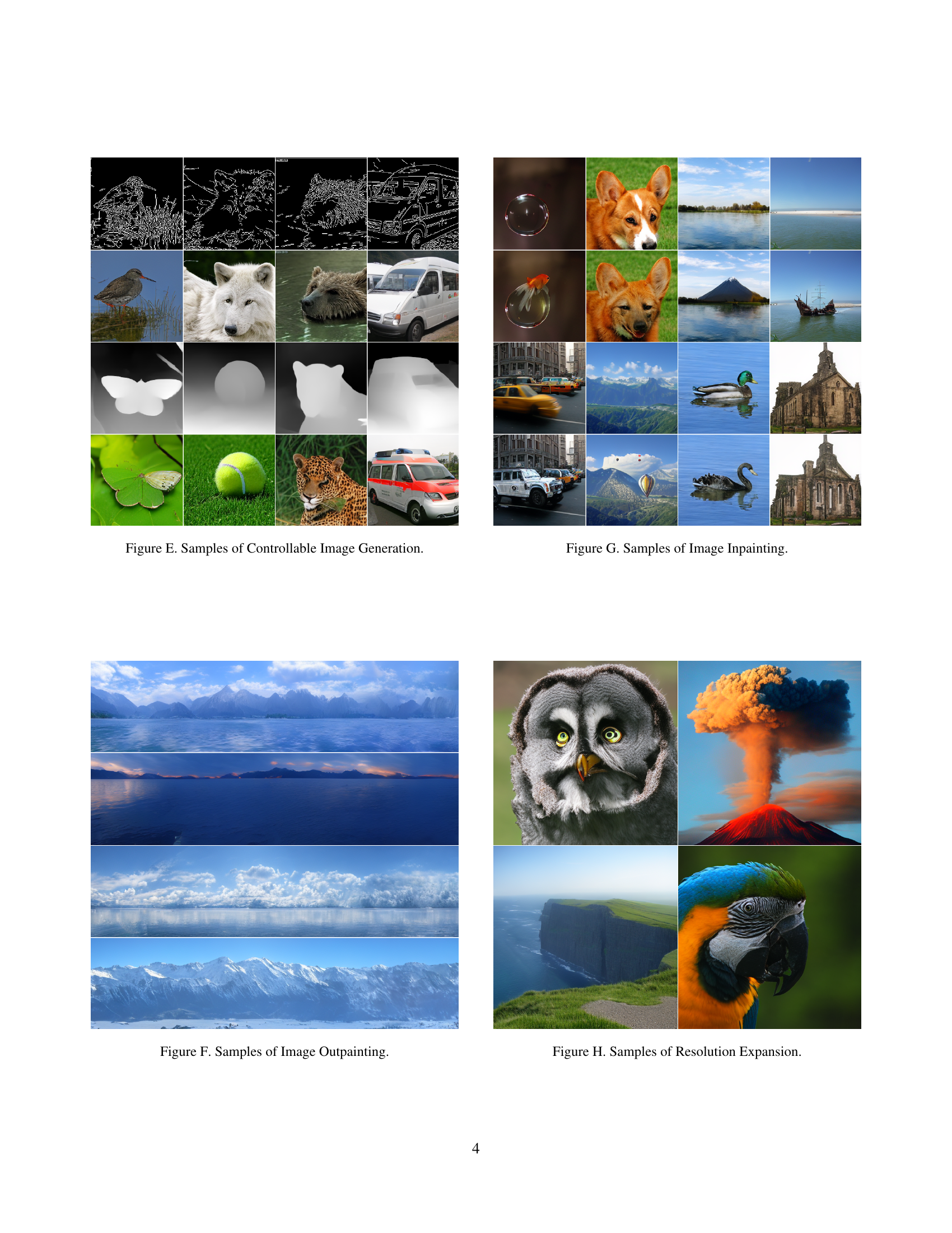
🔼 This figure shows example images generated by the ARPG model under the control of additional information, such as canny edges and depth maps. The model is able to generate images that incorporate these additional inputs, demonstrating its capability for controllable image synthesis. This showcases the flexibility of the ARPG approach in creating images beyond simple class-conditional generation.
read the caption
(b) Controllable Image Generation
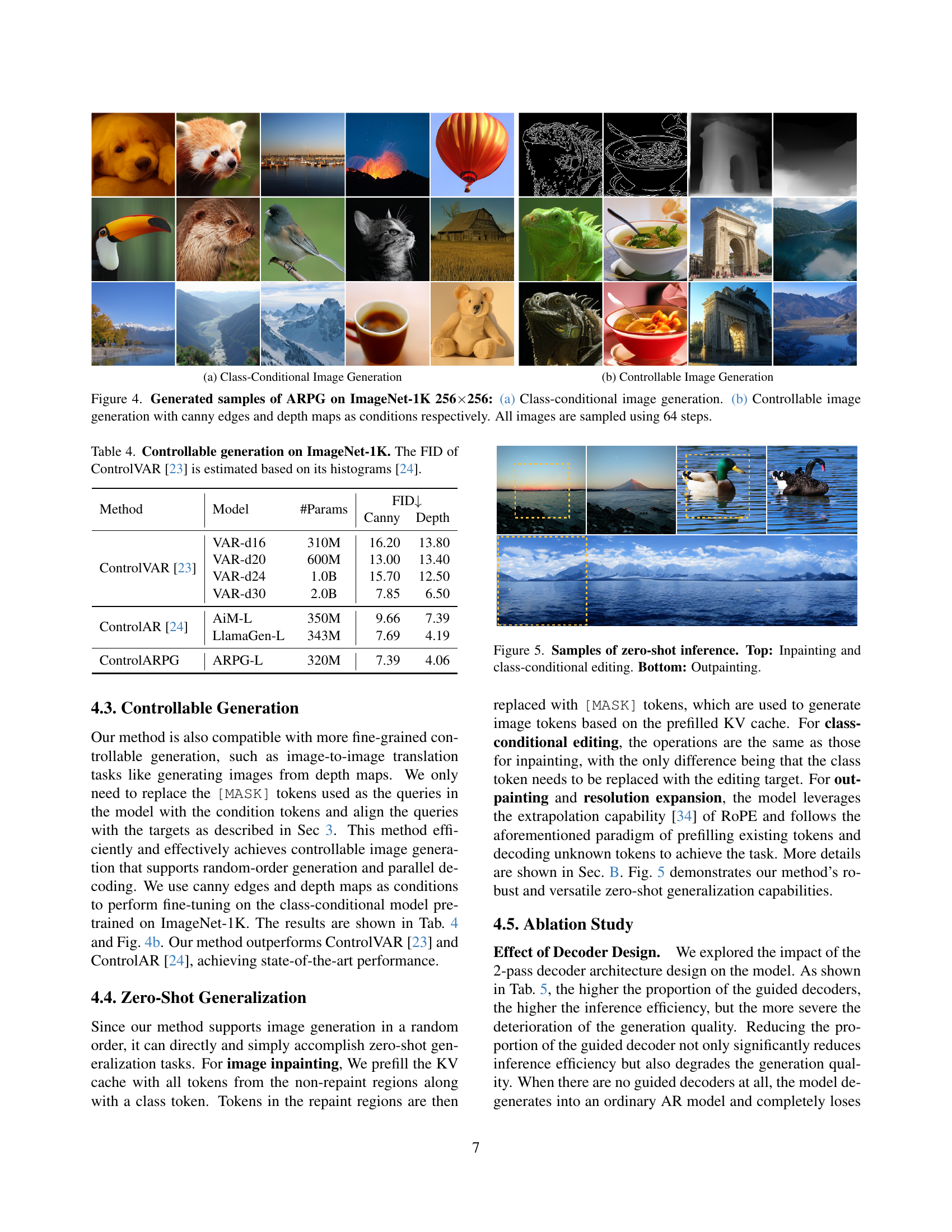
🔼 Figure 4 presents example images generated by the ARPG model. Subfigure 4(a) showcases class-conditional image generation, where the model generates images based solely on a given class label. Subfigure 4(b) demonstrates controllable image generation, in which the model generates images guided by both a class label and additional conditional information, specifically canny edges and depth maps. This illustrates the model’s ability to incorporate external cues to influence the image synthesis process. All images shown were generated with 64 sampling steps.
read the caption
Figure 4: Generated samples of ARPG on ImageNet-1K 256×\times×256: 4(a) Class-conditional image generation. 4(b) Controllable image generation with canny edges and depth maps as conditions respectively. All images are sampled using 64 steps.

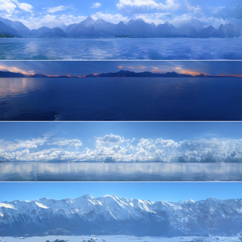
🔼 Figure 5 showcases the model’s zero-shot capabilities on image manipulation tasks without explicit training. The top row demonstrates inpainting (filling missing parts of an image) and class-conditional editing (modifying an existing image based on a class label). The bottom row shows outpainting (extending an image beyond its original boundaries). This highlights the model’s ability to generalize to various tasks beyond the standard image generation.
read the caption
Figure 5: Samples of zero-shot inference. Top: Inpainting and class-conditional editing. Bottom: Outpainting.

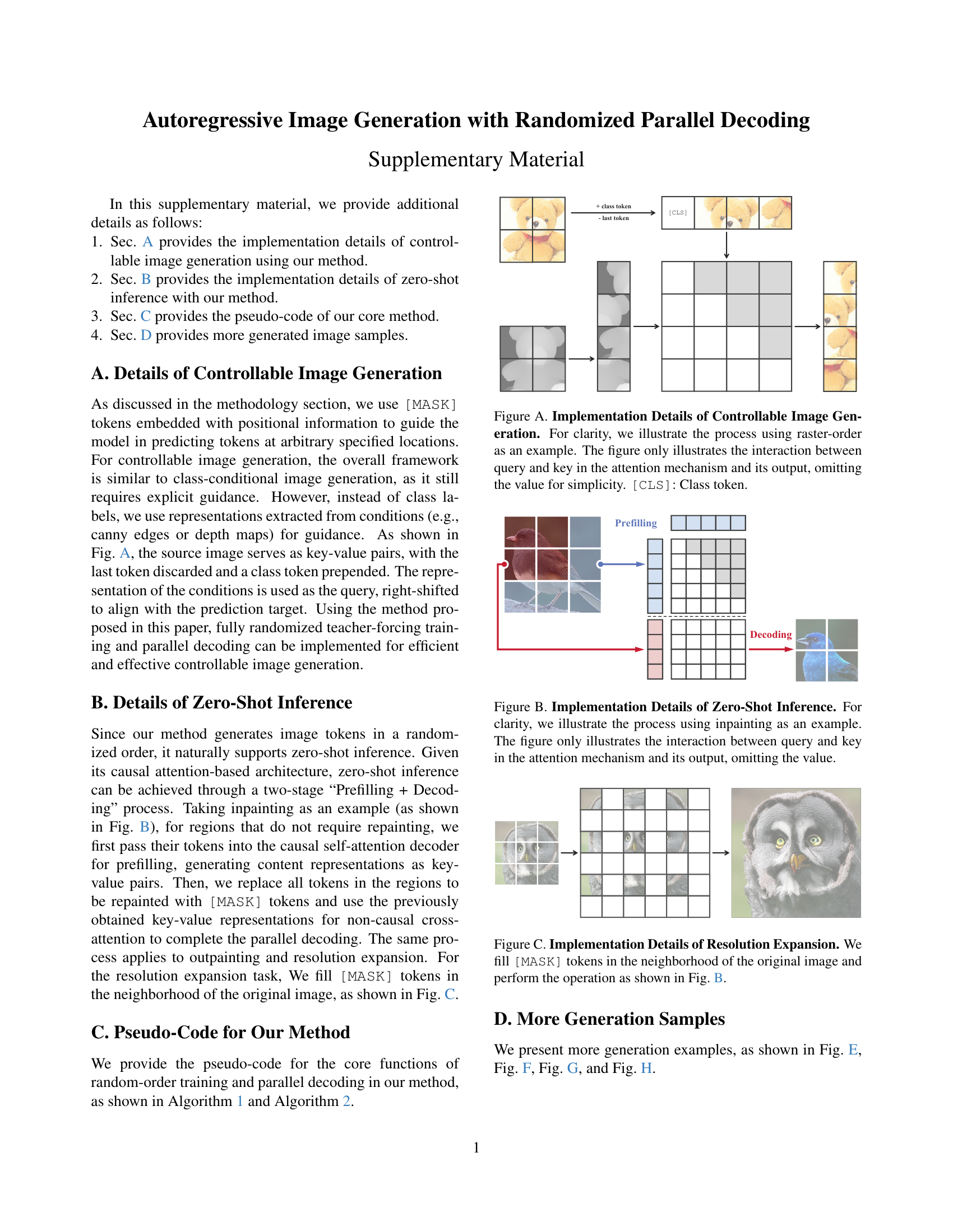
🔼 Figure A illustrates the process of controllable image generation using the ARPG model. It focuses on how the model handles the interaction between queries and keys in the attention mechanism, specifically highlighting how these elements guide the generation process. To simplify the illustration, raster-order generation is used as an example, and the ‘value’ component of the attention mechanism is omitted. The class token ([CLS]) is also shown.
read the caption
Figure A: Implementation Details of Controllable Image Generation. For clarity, we illustrate the process using raster-order as an example. The figure only illustrates the interaction between query and key in the attention mechanism and its output, omitting the value for simplicity. [CLS]: Class token.
More on tables
| Type | Model | Parameters | Steps | Throughput | Memory | FID | IS | Precision | Recall |
| Diffusion | LDM-4 [31] | 400 M | 250 | 0.83 it/s | 5.71 GB | 3.60 | 247.7 | - | - |
| DiT-L/2 [26] | 458 M | 250 | 1.32 it/s | 1.62 GB | 5.02 | 167.2 | 0.75 | 0.57 | |
| DiT-XL/2 [26] | 675 M | 250 | 0.91 it/s | 2.14 GB | 2.27 | 278.2 | 0.83 | 0.57 | |
| Mask | MaskGIT [2] | 227 M | 8 | 46.18 it/s | 1.71 GB | 6.18 | 182.1 | 0.80 | 0.51 |
| MAR-B [22] | 208 M | 100 | 1.71 it/s | 1.47 GB | 2.31 | 281.7 | 0.82 | 0.57 | |
| MAR-L [22] | 479 M | 100 | 1.27 it/s | 2.32 GB | 1.78 | 296.0 | 0.81 | 0.60 | |
| VAR | VAR-d16 [39] | 310 M | 10 | 114.42 it/s | 10.97 GB | 3.30 | 274.4 | 0.84 | 0.51 |
| VAR-d20 [39] | 600 M | 10 | 73.65 it/s | 16.06 GB | 2.57 | 302.6 | 0.83 | 0.56 | |
| VAR-d24 [39] | 1.0 B | 10 | 48.90 it/s | 22.43 GB | 2.09 | 312.9 | 0.82 | 0.59 | |
| AR (Raster) | VQGAN-re [7] | 1.4 B | 256 | 5.92 it/s | 15.15 GB | 5.20 | 280.3 | - | - |
| RQ-Trans.-re [19] | 3.8 B | 64 | 11.63 it/s | 18.43 GB | 3.80 | 323.7 | - | - | |
| LlamaGen-L [35] | 343 M | 576 | 4.33 it/s | 10.23 GB | 3.07 | 256.1 | 0.83 | 0.52 | |
| LlamaGen-XL [35] | 775 M | 576 | 2.46 it/s | 17.11 GB | 2.62 | 244.1 | 0.80 | 0.57 | |
| LlamaGen-XXL [35] | 1.4 B | 576 | 1.58 it/s | 26.22 GB | 2.62 | 244.1 | 0.80 | 0.57 | |
| PAR-L [44] | 343 M | 147 | 14.77 it/s | 10.25 GB | 3.76 | 218.9 | 0.81 | 0.60 | |
| PAR-XL [44] | 775 M | 147 | 7.91 it/s | 17.13 GB | 2.61 | 259.2 | 0.80 | 0.62 | |
| PAR-XXL [44] | 1.4 B | 147 | 5.23 it/s | 26.25 GB | 2.35 | 263.2 | 0.80 | 0.62 | |
| AiM-L [20] | 350 M | 256 | 26.47 it/s | 4.94 GB | 2.83 | 244.6 | 0.82 | 0.55 | |
| AiM-XL [20] | 763 M | 256 | 18.68 it/s | 7.25 GB | 2.56 | 257.2 | 0.82 | 0.57 | |
| RAR-L [50] | 461 M | 256 | 12.08 it/s | 6.37 GB | 1.70 | 299.5 | 0.81 | 0.60 | |
| RAR-XL [50] | 955 M | 256 | 8.00 it/s | 10.55 GB | 1.50 | 306.9 | 0.80 | 0.62 | |
| AR (Random) | RandAR-L [25] | 343 M | 88 | 25.30 it/s | 7.32 GB | 2.55 | 288.8 | 0.81 | 0.58 |
| RandAR-XL [25] | 775 M | 88 | 15.51 it/s | 13.52 GB | 2.25 | 317.8 | 0.80 | 0.60 | |
| RandAR-XXL [25] | 1.4 B | 88 | 10.46 it/s | 21.77 GB | 2.15 | 322.0 | 0.79 | 0.62 | |
| AR (Random) | ARPG-L | 320 M | 32 | 113.01 it/s | 2.54 GB | 2.44 | 291.7 | 0.82 | 0.55 |
| ARPG-L | 320 M | 64 | 62.12 it/s | 2.43 GB | 2.44 | 287.1 | 0.82 | 0.55 | |
| ARPG-XL | 719 M | 64 | 35.89 it/s | 4.48 GB | 2.10 | 331.0 | 0.79 | 0.61 | |
| ARPG-XXL | 1.3 B | 64 | 25.39 it/s | 7.31 GB | 1.94 | 339.7 | 0.81 | 0.59 |
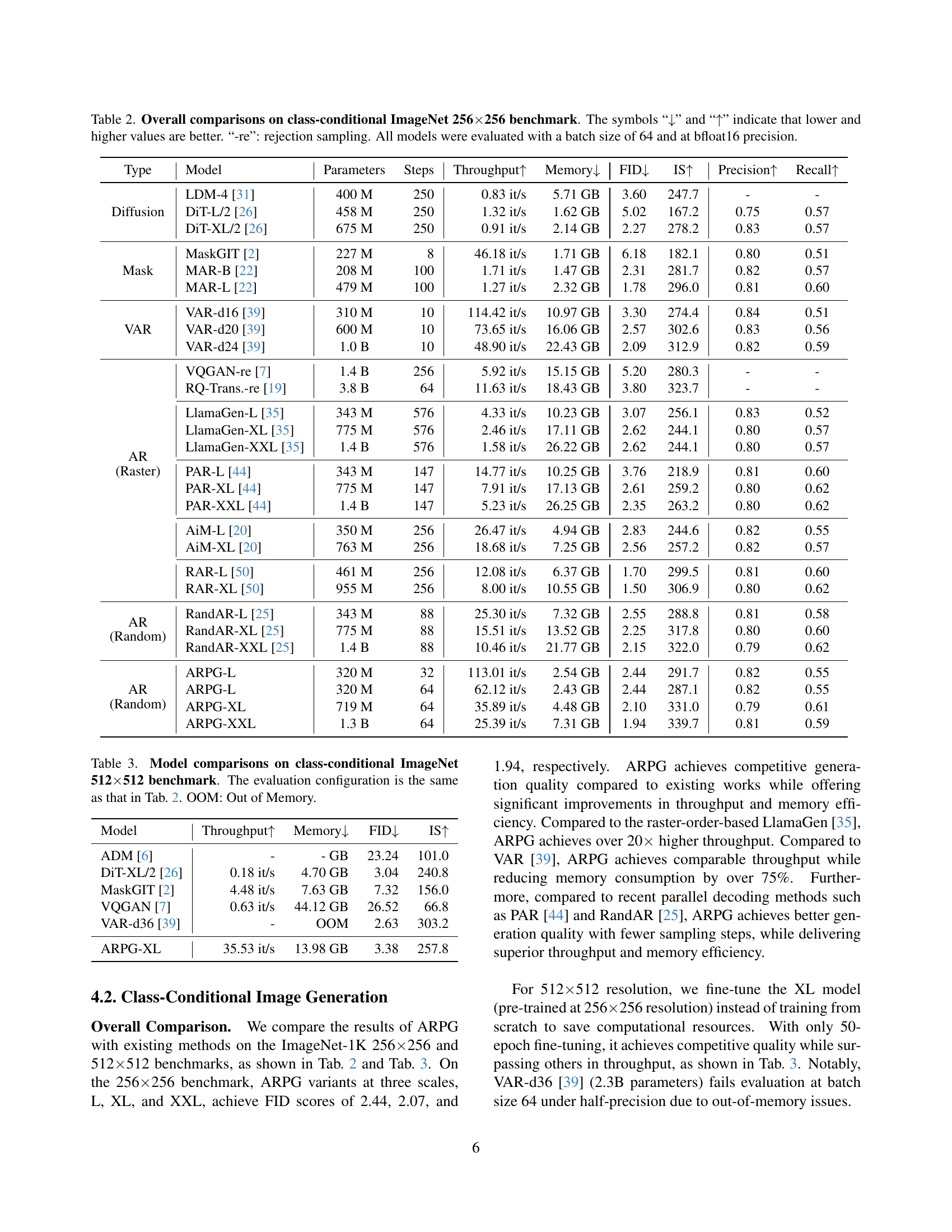
🔼 Table 2 presents a comprehensive comparison of various autoregressive image generation models on the ImageNet 256x256 dataset. The models are categorized into diffusion, masked, and autoregressive models (both raster and random order). For each model, the table shows the number of parameters, the number of generation steps, the image generation throughput (images per second), memory usage (in GB), Fréchet Inception Distance (FID, lower is better, indicating higher image quality), Inception Score (IS, higher is better, indicating better image diversity), precision, and recall. This allows for a direct comparison of model performance across different approaches, highlighting the relative strengths and weaknesses of each method in terms of speed, memory efficiency, and image quality.
read the caption
Table 2: Overall comparisons on class-conditional ImageNet 256×\times×256 benchmark. The symbols “↓↓\downarrow↓” and “↑↑\uparrow↑” indicate that lower and higher values are better. “-re”: rejection sampling. All models were evaluated with a batch size of 64 and at bfloat16 precision.
| Model | Throughput | Memory | FID | IS |
|---|---|---|---|---|
| ADM [6] | - | - GB | 23.24 | 101.0 |
| DiT-XL/2 [26] | 0.18 it/s | 4.70 GB | 3.04 | 240.8 |
| MaskGIT [2] | 4.48 it/s | 7.63 GB | 7.32 | 156.0 |
| VQGAN [7] | 0.63 it/s | 44.12 GB | 26.52 | 66.8 |
| VAR-d36 [39] | - | OOM | 2.63 | 303.2 |
| ARPG-XL | 35.53 it/s | 13.98 GB | 3.38 | 257.8 |
🔼 This table presents a comparison of different autoregressive image generation models on the ImageNet 512x512 dataset for class-conditional image generation. The models are evaluated using FID (Fréchet Inception Distance) score, Inception Score (IS), and throughput (images per second). Memory usage (in GB) is also reported. The metrics are used to assess the quality and efficiency of each model. The same evaluation configuration as Table 2 was used. ‘OOM’ indicates that a model ran out of memory during evaluation.
read the caption
Table 3: Model comparisons on class-conditional ImageNet 512×\times×512 benchmark. The evaluation configuration is the same as that in Tab. 2. OOM: Out of Memory.
| Method | Model | #Params | FID | |
| Canny | Depth | |||
| ControlVAR [23] | VAR-d16 | 310M | 16.20 | 13.80 |
| VAR-d20 | 600M | 13.00 | 13.40 | |
| VAR-d24 | 1.0B | 15.70 | 12.50 | |
| VAR-d30 | 2.0B | 7.85 | 6.50 | |
| ControlAR [24] | AiM-L | 350M | 9.66 | 7.39 |
| LlamaGen-L | 343M | 7.69 | 4.19 | |
| ControlARPG | ARPG-L | 320M | 7.39 | 4.06 |
🔼 This table presents a comparison of different models’ performance on controllable image generation tasks using the ImageNet-1K dataset. It shows the Fréchet Inception Distance (FID) scores, a measure of generated image quality, for various models when generating images conditioned on canny edges and depth maps. The FID score for the ControlVAR model is estimated from its histogram data, as explicitly noted. Lower FID scores indicate better image quality.
read the caption
Table 4: Controllable generation on ImageNet-1K. The FID of ControlVAR [23] is estimated based on its histograms [24].
| Description | Parameters | Layers | Randomize | Parallelize | Steps | Throughput | Memory | FID | IS |
| ARPG-L | 320 M | 12 + 12 | 64 | 62.12 it/s | 2.43 GB | 3.51 | 282.7 | ||
| + Longer Training | 320 M | 12 + 12 | 64 | 62.12 it/s | 2.43 GB | 2.44 | 287.1 | ||
| + w/o Shared KV | 343 M | 12 + 12 | 64 | 48.02 it/s | 3.83 GB | 2.37 | 299.7 | ||
| Fewer Guided Decoder | 332 M | 18 + 6 | 64 | 50.72 it/s | 3.19 GB | 3.82 | 223.0 | ||
| More Guided Decoder | 307 M | 6 + 18 | 64 | 66.11 it/s | 1.67 GB | 3.51 | 242.5 | ||
| w/o Guided Decoder | 343 M | 24 + 0 | 256 | 11.70 it/s | 4.96 GB | 90 | 50 | ||
| Guided Decoder Only | 295 M | 0 + 24 | 64 | 72.26 it/s | 0.91 GB | 4.57 | 255.9 |
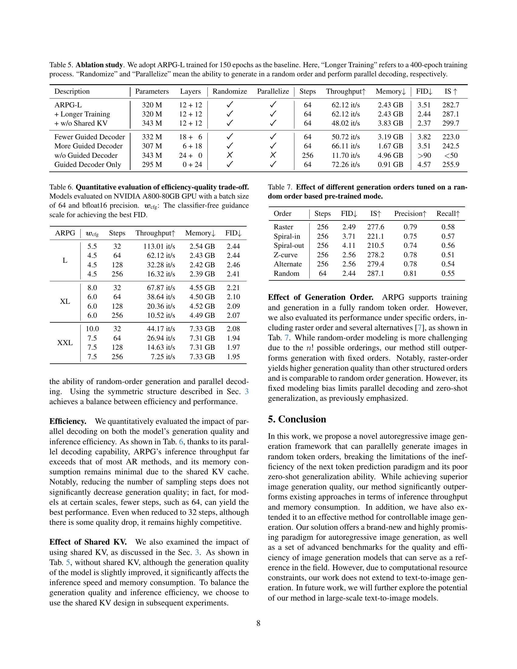
🔼 This ablation study investigates the impact of various design choices on ARPG-L, a model trained for 150 epochs. The baseline model’s performance is compared against variations including extending training to 400 epochs, removing the shared key-value cache, adjusting the number of guided decoder layers, and removing or solely using guided decoder layers. The table assesses each variation across parameters, layers, random generation capability, parallel decoding capability, number of sampling steps, throughput, memory usage, FID score, and Inception Score (IS) to determine the effects on both efficiency and image generation quality.
read the caption
Table 5: Ablation study. We adopt ARPG-L trained for 150 epochs as the baseline. Here, “Longer Training” refers to a 400-epoch training process. “Randomize” and “Parallelize” mean the ability to generate in a random order and perform parallel decoding, respectively.
| ARPG | Steps | Throughput | Memory | FID | |
|---|---|---|---|---|---|
| L | 5.5 | 32 | 113.01 it/s | 2.54 GB | 2.44 |
| 4.5 | 64 | 62.12 it/s | 2.43 GB | 2.44 | |
| 4.5 | 128 | 32.28 it/s | 2.42 GB | 2.46 | |
| 4.5 | 256 | 16.32 it/s | 2.39 GB | 2.41 | |
| XL | 8.0 | 32 | 67.87 it/s | 4.55 GB | 2.21 |
| 6.0 | 64 | 38.64 it/s | 4.50 GB | 2.10 | |
| 6.0 | 128 | 20.36 it/s | 4.52 GB | 2.09 | |
| 6.0 | 256 | 10.52 it/s | 4.49 GB | 2.07 | |
| XXL | 10.0 | 32 | 44.17 it/s | 7.33 GB | 2.08 |
| 7.5 | 64 | 26.94 it/s | 7.31 GB | 1.94 | |
| 7.5 | 128 | 14.63 it/s | 7.31 GB | 1.97 | |
| 7.5 | 256 | 7.25 it/s | 7.33 GB | 1.95 |
🔼 Table 6 presents a quantitative analysis of the trade-off between efficiency and image generation quality for different model configurations. The models were evaluated using an NVIDIA A800-80GB GPU, a batch size of 64, and bfloat16 precision. The table shows how various settings (model size, number of steps, and classifier-free guidance scale (wcfg)) impact the FID (Fréchet Inception Distance) score, throughput (images/second), memory usage (in GB), and Inception Score (IS). The wcfg value represents the scaling factor used to achieve the best FID for each model configuration.
read the caption
Table 6: Quantitative evaluation of efficiency-quality trade-off. Models evaluated on NVIDIA A800-80GB GPU with a batch size of 64 and bfloat16 precision. 𝒘cfgsubscript𝒘cfg\bm{w}_{\text{cfg}}bold_italic_w start_POSTSUBSCRIPT cfg end_POSTSUBSCRIPT: The classifier-free guidance scale for achieving the best FID.
| Order | Steps | FID | IS | Precision | Recall |
|---|---|---|---|---|---|
| Raster | 256 | 2.49 | 277.6 | 0.79 | 0.58 |
| Spiral-in | 256 | 3.71 | 221.1 | 0.75 | 0.57 |
| Spiral-out | 256 | 4.11 | 210.5 | 0.74 | 0.56 |
| Z-curve | 256 | 2.56 | 278.2 | 0.78 | 0.51 |
| Alternate | 256 | 2.56 | 279.4 | 0.78 | 0.54 |
| Random | 64 | 2.44 | 287.1 | 0.81 | 0.55 |
🔼 This table presents the results of an ablation study that explores the impact of different image generation orders on a model pre-trained with a random generation order. The study compares the model’s performance (FID, IS, Precision, Recall) when generating images using various orders, including raster scan, spiral-in, spiral-out, Z-curve, alternate, and the random order used during pre-training. This helps understand how the chosen generation order affects the quality and efficiency of the model’s output.
read the caption
Table 7: Effect of different generation orders tuned on a random order based pre-trained mode.
Full paper#