TL;DR#
Normalization layers are a staple in modern neural networks, believed to be vital for good performance. They help optimization, stabilize convergence, and are deemed indispensable. However, recent architectures focus on replacing attention or convolution while still keeping normalization layers. This paper challenges the necessity of normalization by introducing Dynamic Tanh (DyT) as a simple alternative.
This paper shows Transformers without normalization are viable. DyT, defined as DyT(x) = tanh(ax) (where ‘a’ is learnable), mimics layer normalization’s S-shaped mapping. DyT-integrated Transformers matched or exceeded normalized versions’ performance across tasks like recognition, generation, & self-supervision, from vision to language. The finding challenges normalization’s necessity and suggests new insights into deep networks.
Key Takeaways#
Why does it matter?#
This paper is important because it challenges the long-held belief that normalization layers are essential in deep networks, potentially simplifying architectures & reducing computational costs. This work can opens new doors for designing & training more efficient deep learning models.
Visual Insights#

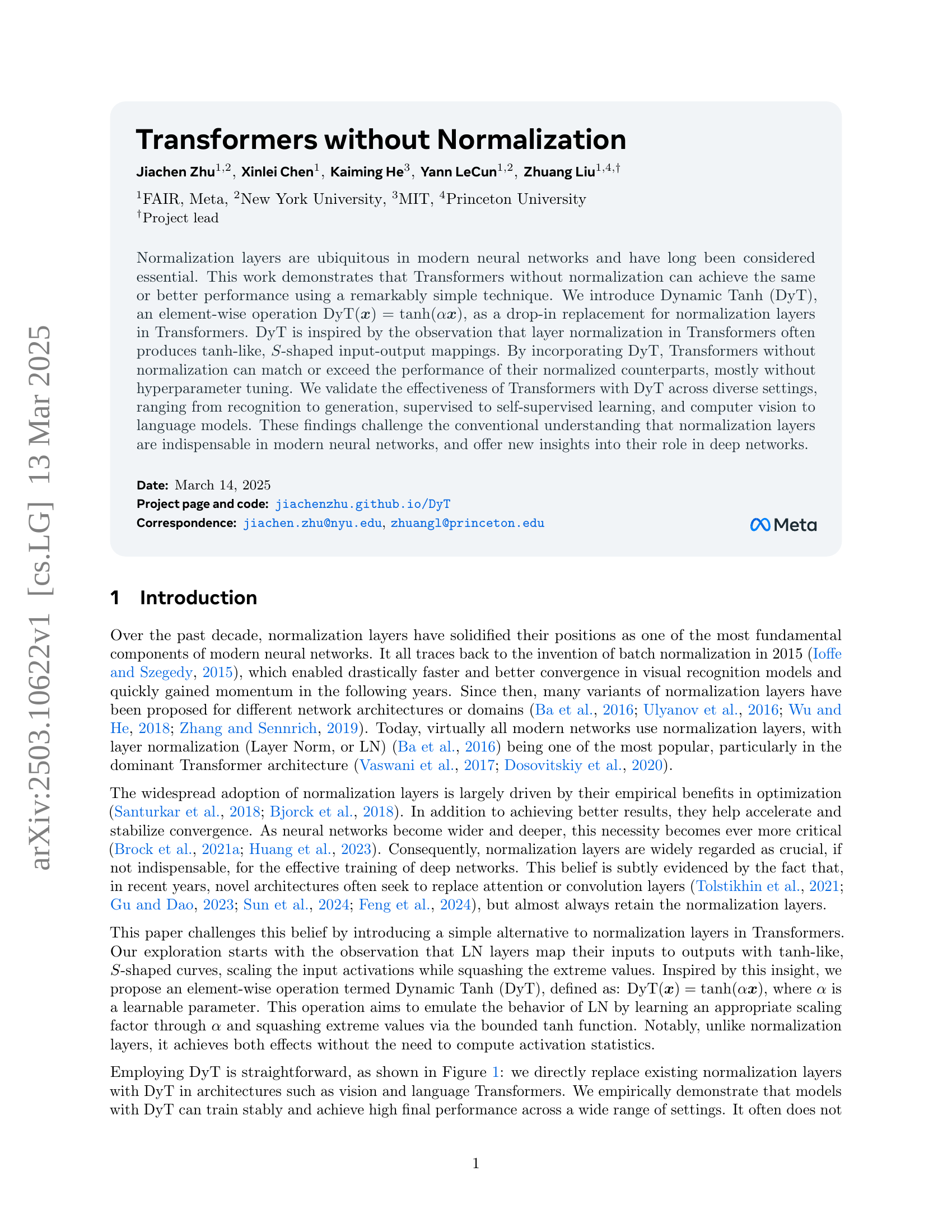
🔼 This figure illustrates the architecture of a standard Transformer block and a modified version incorporating the proposed Dynamic Tanh (DyT) layer. The left panel depicts a traditional Transformer block, highlighting its core components: Attention/Feed-Forward Network (Attention/FFN), Layer Normalization (LN), and scale & shift operations. The right panel shows the integration of the DyT layer as a direct replacement for LN. The DyT layer functions as a learnable element-wise operation, approximating the behavior of LN and RMSNorm (another normalization technique) while omitting the computationally expensive statistical calculations. The caption emphasizes that using DyT instead of LN results in similar or superior performance in Transformers.
read the caption
Figure 1: Left: original Transformer block. Right: block with our proposed Dynamic Tanh (DyT) layer. DyT is a straightforward replacement for commonly used Layer Norm (Ba et al., 2016) (in some cases RMSNorm (Zhang and Sennrich, 2019)) layers. Transformers with DyT match or exceed the performance of their normalized counterparts.
| model | LN | DyT | change |
|---|---|---|---|
| ViT-B | 82.3% | 82.5% | 0.2% |
| ViT-L | 83.1% | 83.6% | 0.5% |
| ConvNeXt-B | 83.7% | 83.7% | - |
| ConvNeXt-L | 84.3% | 84.4% | 0.1% |
🔼 This table presents the top-1 accuracy results of image classification on the ImageNet-1K dataset for four different models: ViT-B, ViT-L, ConvNeXt-B, and ConvNeXt-L. Each model was trained using two different normalization methods: Layer Normalization (LN) and Dynamic Tanh (DyT). The table shows that the performance with DyT is either on par with or superior to the performance achieved with LN. This comparison is made across various model sizes, demonstrating the effectiveness and generalizability of DyT.
read the caption
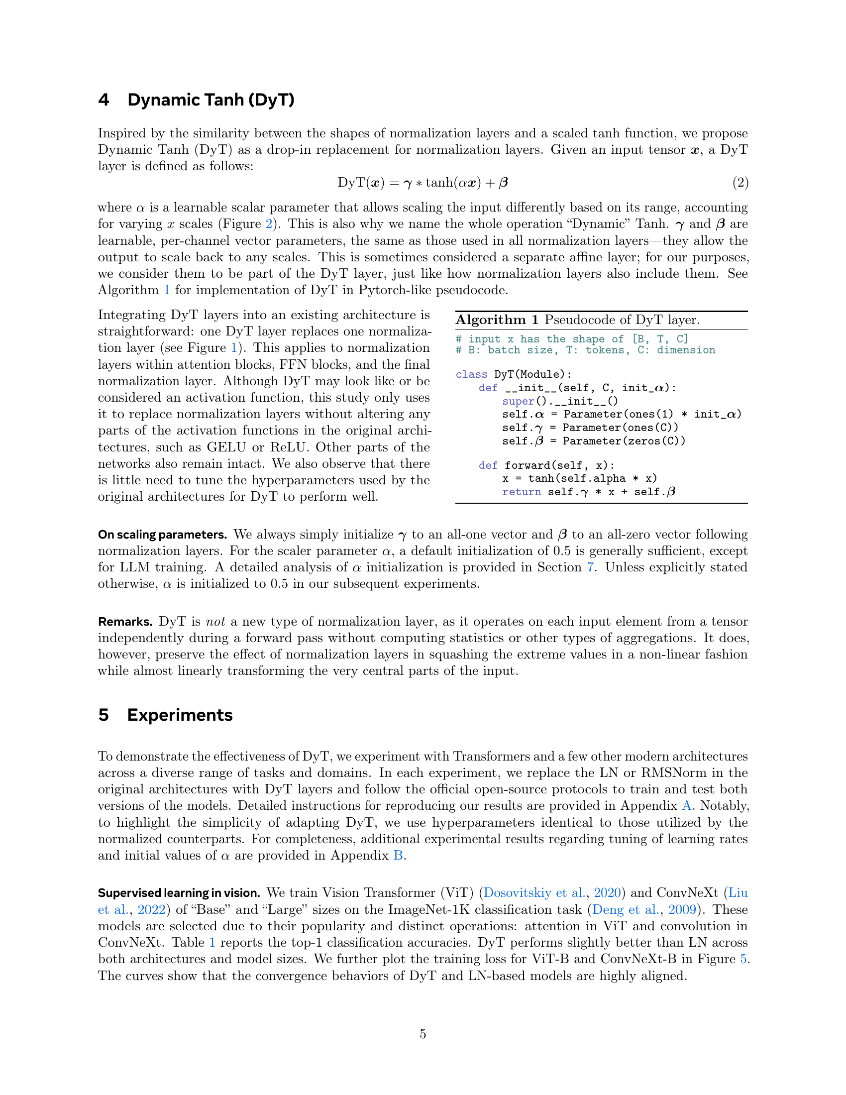
Table 1: Supervised classification accuracy on ImageNet-1K. DyT achieves better or similar performance than LN across both architectures and model sizes.
In-depth insights#
DyT: How it works#
Dynamic Tanh (DyT) operates as a drop-in replacement for normalization layers, primarily in Transformers. It introduces a learnable scaling factor alpha that adjusts the input activation range before squashing extreme values via a tanh function. Unlike normalization layers which compute statistics across tokens, DyT operates element-wise without aggregation, emulating normalization’s S-shaped input-output mapping with a scaled tanh. This approach offers simplicity and potential efficiency gains.
Beyond LayerNorm#
Moving beyond LayerNorm (LN) is a compelling direction for neural network research. While LN has become a staple, especially in Transformers, its limitations warrant exploration of alternatives. DyT offers a fresh perspective by directly addressing LN’s behavior, i.e., mapping to tanh-like curves, which is innovative. It opens a pathway to understand, whether normalization’s benefits stem solely from statistical normalization, or from the non-linear element-wise squashing, and or from learning scaling paramters. DyT’s simplicity is an asset. It reduces computational overhead, and potentially improves inference speed as suggested. This can be valuable for resource-constrained environments. Its drop-in nature also makes experimentation easy. If DyT can achieve comparable or superior performance, it challenges the necessity of complex normalization. Further, this motivates rethinking network architectures from the ground up, rather than relying on norm by default.
No-Norm ViTs/DiTs#
Normalization layers are ubiquitous in Vision Transformers (ViTs) and Diffusion Transformers (DiTs), yet the paper challenges their necessity. The concept of “No-Norm ViTs/DiTs” suggests eliminating normalization layers while maintaining or improving performance. The paper introduces Dynamic Tanh (DyT) as a substitute, emulating the behavior of normalization. This substitution presents potential benefits like reduced computational overhead and simplification of network architecture. A deeper question explored might be whether normalization’s primary role is simply activation scaling and stabilization, which DyT effectively addresses. By challenging the necessity of normalization layers, this work could potentially lead to more efficient and interpretable network designs in the future for both ViTs and DiTs.
Model Scaling Laws#
Model scaling laws are crucial for understanding the relationship between model size, dataset size, and performance. Intuitively, larger models trained on more data perform better, but scaling laws quantify this relationship precisely. These laws often express performance as a power-law function of model size, indicating diminishing returns as models grow. Understanding these laws allows for efficient resource allocation by predicting the optimal model size for a given dataset and computational budget. Deviations from scaling laws can also reveal architectural inefficiencies or dataset biases. While the initial focus was on language models, scaling laws are now being investigated in other domains like computer vision and reinforcement learning. Extending and refining these laws remains an active area of research, particularly in understanding the role of architectural innovations and the impact of data quality on scaling behavior.
BN limitations?#
While Batch Normalization (BN) has been foundational, it has limitations. BN’s reliance on batch statistics can be problematic with small batch sizes, leading to inaccurate normalization and reduced performance. Furthermore, BN’s effectiveness diminishes in recurrent neural networks (RNNs) due to the varying statistics across time steps. Additionally, BN introduces dependencies between samples within a batch, which can be undesirable in certain applications like reinforcement learning. There is the computational overhead associated with calculating and storing batch statistics during training, as well as the need for separate handling during inference. The above can also limit the architectural flexibility, since BN can interfere with certain network designs and training techniques.
More visual insights#
More on figures
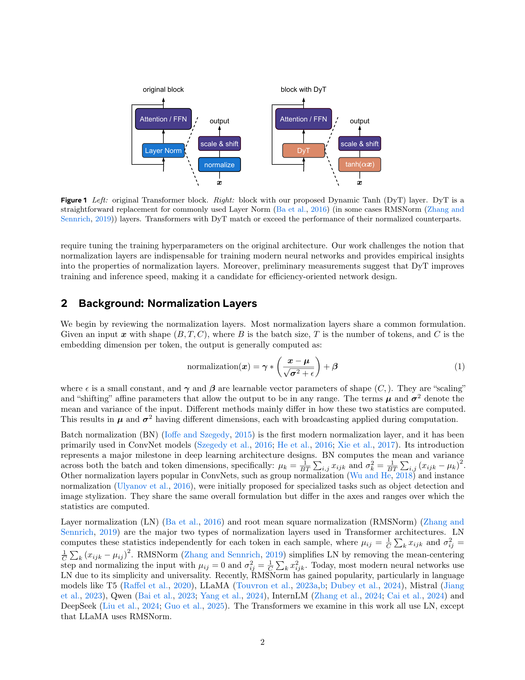
🔼 This figure displays scatter plots visualizing the relationship between input and output values for selected layer normalization (LN) layers within three different Transformer models: Vision Transformer (ViT), wav2vec 2.0, and Diffusion Transformer (DiT). For each model, four different LN layers are represented. The x-axis represents the input values to the LN layer, and the y-axis shows the corresponding output values (before the affine transformation within the LN layer). The plots reveal that the input-output mappings of the LN layers often exhibit a characteristic S-shaped or tanh-like curve, particularly in deeper layers, which is a key observation in the paper that motivates the proposed Dynamic Tanh (DyT) method as a more efficient and effective replacement for the LN layer.
read the caption
Figure 2: Output vs. input of selected layer normalization (LN) layers in Vision Transformer (ViT) (Dosovitskiy et al., 2020), wav2vec 2.0 (a Transformer model for speech) (Baevski et al., 2020), and Diffusion Transformer (DiT) (Peebles and Xie, 2023). We sample a mini-batch of samples and plot the input / output values of four LN layers in each model. The outputs are before the affine transformation in LN. The S𝑆Sitalic_S-shaped curves highly resemble that of a tanh function (see Figure 3). The more linear shapes in earlier layers can also be captured by the center part of a tanh curve. This motivates us to propose Dynamic Tanh (DyT) as a replacement, with a learnable scaler α𝛼\alphaitalic_α to account for different scales on the x𝑥xitalic_x axis.

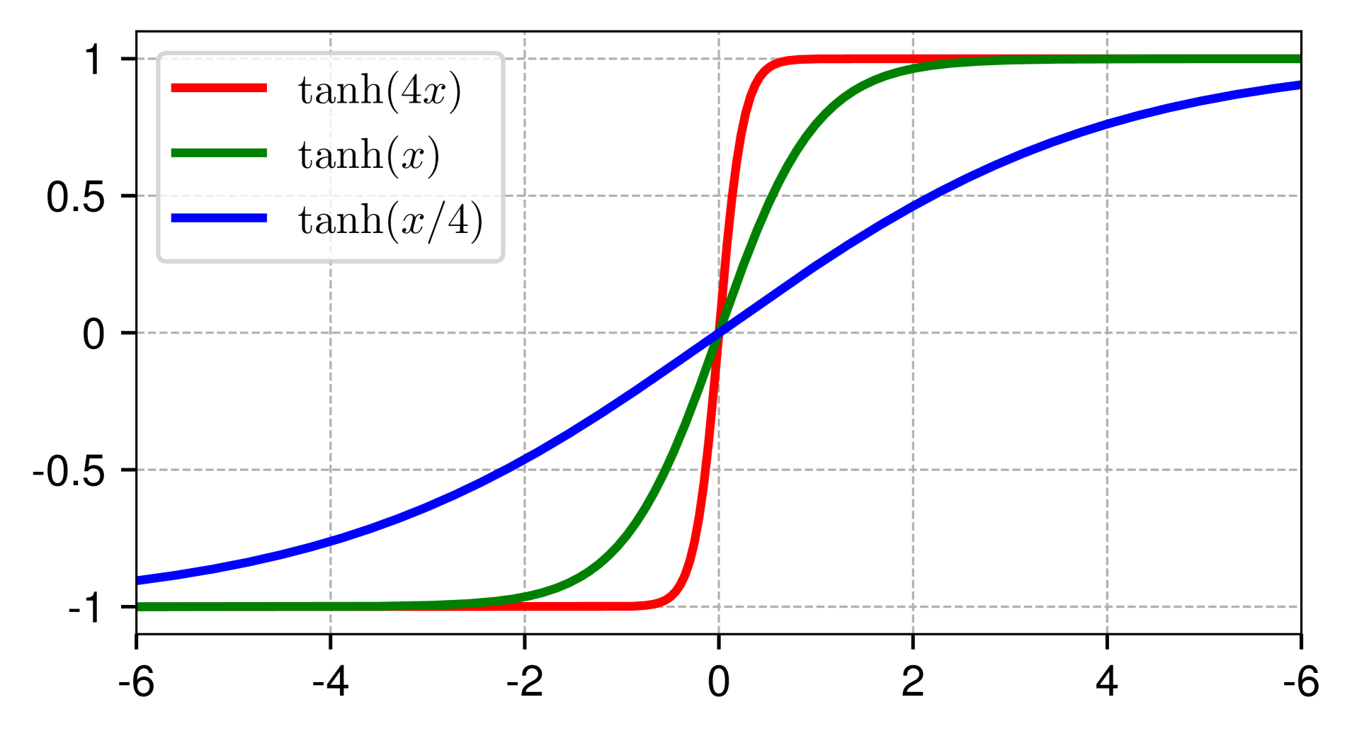
🔼 This figure shows plots of the function y = tanh(αx) for three different values of α (alpha). The parameter α controls the steepness of the curve. A larger α value results in a steeper curve, while a smaller α value results in a shallower curve. The tanh function itself is a sigmoid function that maps values from negative infinity to positive infinity to a range between -1 and 1. This function’s shape is similar to the input-output relationship observed in layer normalization (LN) layers of Transformer models, which inspired the use of the Dynamic Tanh (DyT) function in the paper. The figure visually illustrates how the DyT function with its learnable parameter α can mimic the behavior of LN layers in squashing extreme values while maintaining a relatively linear response in the central region.
read the caption
Figure 3: tanh(αx)𝛼𝑥\tanh(\alpha x)roman_tanh ( italic_α italic_x ) with three different α𝛼\alphaitalic_α values.

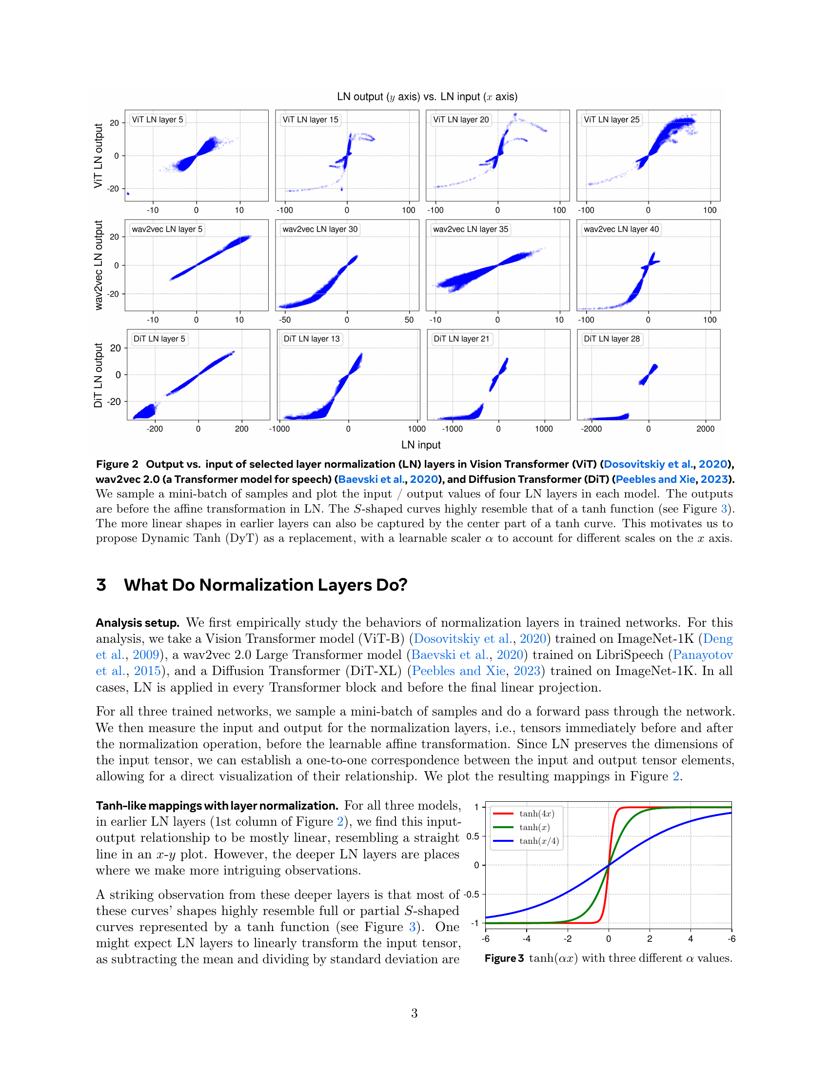
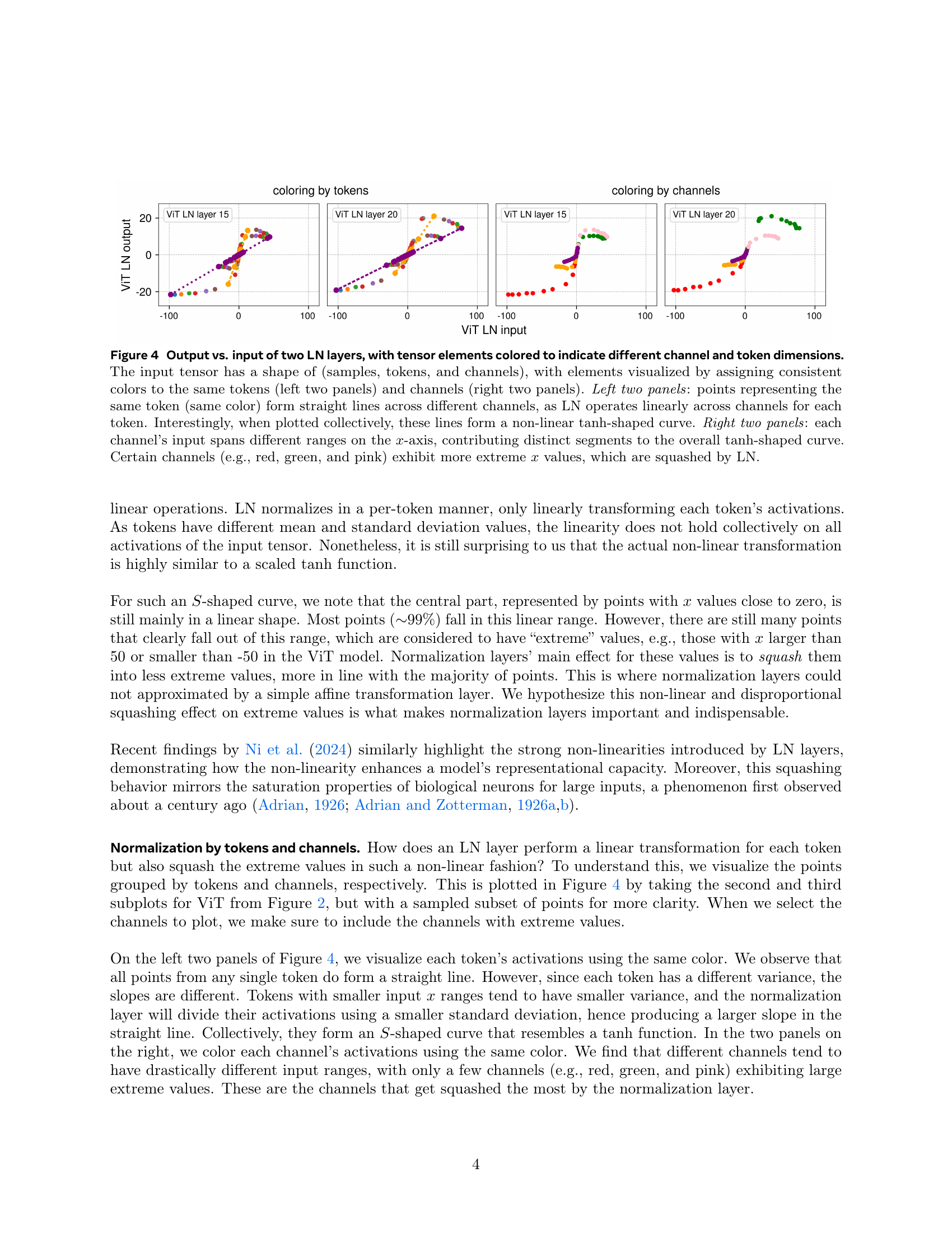
🔼 Figure 4 visualizes the input-output relationships of layer normalization (LN) layers in a vision transformer model. The plots show how LN processes inputs by separating and handling data across token and channel dimensions. The left two panels highlight that LN acts linearly across channels for each token. Individual tokens (same color) plot as straight lines. However, the collection of these lines creates a nonlinear, S-shaped (tanh-like) curve. The right two panels illustrate the different input ranges across individual channels. Some channels have more extreme input values that are squashed by LN, resulting in the S-shaped curve. This visualization clarifies LN’s dual nature of linear processing per token and nonlinear squashing of extremes across all channels.
read the caption
Figure 4: Output vs. input of two LN layers, with tensor elements colored to indicate different channel and token dimensions. The input tensor has a shape of (samples, tokens, and channels), with elements visualized by assigning consistent colors to the same tokens (left two panels) and channels (right two panels). Left two panels: points representing the same token (same color) form straight lines across different channels, as LN operates linearly across channels for each token. Interestingly, when plotted collectively, these lines form a non-linear tanh-shaped curve. Right two panels: each channel’s input spans different ranges on the x𝑥xitalic_x-axis, contributing distinct segments to the overall tanh-shaped curve. Certain channels (e.g., red, green, and pink) exhibit more extreme x𝑥xitalic_x values, which are squashed by LN.

🔼 This figure displays the training loss curves for two different models, Vision Transformer (ViT-B) and ConvNeXt-B, both trained using two different normalization methods: Layer Normalization (LN) and Dynamic Tanh (DyT). The curves for both models and both normalization techniques show remarkably similar patterns and rates of convergence, suggesting a strong similarity in how these different methods affect the training process. This implies that DyT, a much simpler normalization technique, might effectively replicate the behavior and benefits of the more complex LN during training.
read the caption
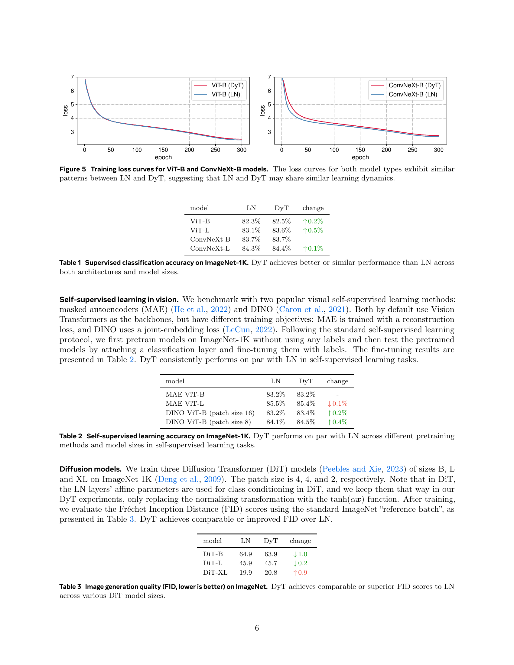
Figure 5: Training loss curves for ViT-B and ConvNeXt-B models. The loss curves for both model types exhibit similar patterns between LN and DyT, suggesting that LN and DyT may share similar learning dynamics.

🔼 This figure displays the training loss curves for four different sizes of the LLaMA large language model (LLaMA 7B, 13B, 34B, and 70B) during pretraining. Each model size is shown with two curves: one using RMSNorm (the original normalization method) and another using the proposed DyT (Dynamic Tanh) method. The closeness of the curves for each model size shows that DyT achieves comparable performance to RMSNorm during training, regardless of model size.
read the caption
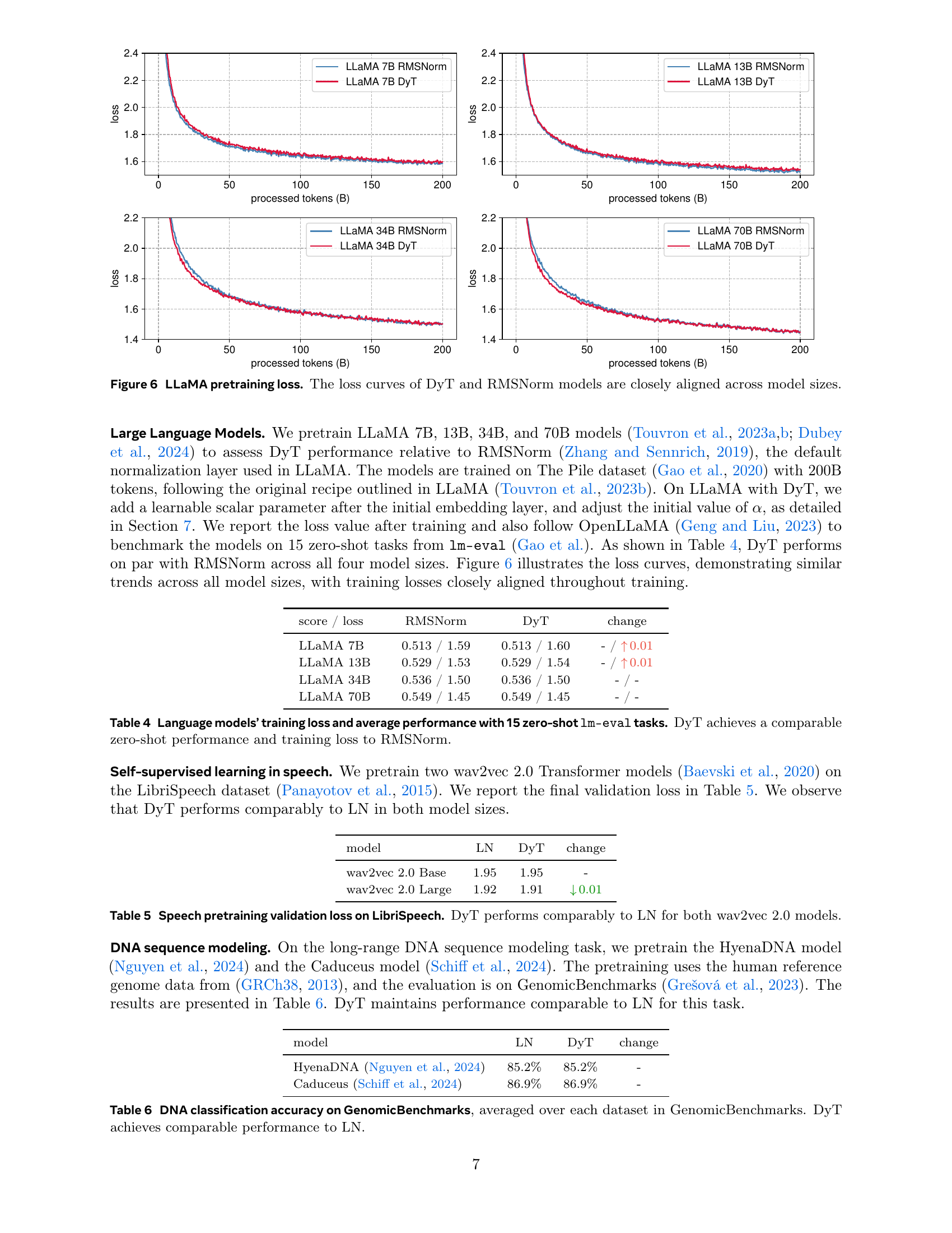
Figure 6: LLaMA pretraining loss. The loss curves of DyT and RMSNorm models are closely aligned across model sizes.
More on tables
| model | LN | DyT | change |
|---|---|---|---|
| MAE ViT-B | 83.2% | 83.2% | - |
| MAE ViT-L | 85.5% | 85.4% | 0.1% |
| DINO ViT-B (patch size 16) | 83.2% | 83.4% | 0.2% |
| DINO ViT-B (patch size 8) | 84.1% | 84.5% | 0.4% |
🔼 This table presents the results of self-supervised learning experiments on the ImageNet-1K dataset. Two popular self-supervised learning methods, Masked Autoencoders (MAE) and DINO, were used, each with Vision Transformer backbones of varying sizes. The table compares the top-1 classification accuracy achieved after fine-tuning the pre-trained models with both Layer Normalization (LN) and Dynamic Tanh (DyT). This demonstrates that DyT achieves comparable performance to LN across different model sizes and self-supervised learning methods.
read the caption
Table 2: Self-supervised learning accuracy on ImageNet-1K. DyT performs on par with LN across different pretraining methods and model sizes in self-supervised learning tasks.
| model | LN | DyT | change |
|---|---|---|---|
| DiT-B | 64.9 | 63.9 | 1.0 |
| DiT-L | 45.9 | 45.7 | 0.2 |
| DiT-XL | 19.9 | 20.8 | 0.9 |
🔼 This table presents the Fréchet Inception Distance (FID) scores, a metric for evaluating the quality of generated images, for three different sizes of the Diffusion Transformer (DiT) model. The models were trained on the ImageNet-1K dataset. Lower FID scores indicate better image generation quality. The table compares the FID scores achieved by models using layer normalization (LN) with those using the proposed Dynamic Tanh (DyT) as a replacement for LN. The results demonstrate that DyT achieves comparable or superior performance compared to LN across all model sizes.
read the caption
Table 3: Image generation quality (FID, lower is better) on ImageNet. DyT achieves comparable or superior FID scores to LN across various DiT model sizes.
| score / loss | RMSNorm | DyT | change |
|---|---|---|---|
| LLaMA 7B | 0.513 / 1.59 | 0.513 / 1.60 | - / 0.01 |
| LLaMA 13B | 0.529 / 1.53 | 0.529 / 1.54 | - / 0.01 |
| LLaMA 34B | 0.536 / 1.50 | 0.536 / 1.50 | - / - |
| LLaMA 70B | 0.549 / 1.45 | 0.549 / 1.45 | - / - |
🔼 This table presents a comparison of the performance of large language models (LLaMs) using either RMSNorm or DyT normalization. It shows the training loss and average performance across 15 zero-shot tasks from the lm-eval benchmark. The results demonstrate that DyT achieves comparable performance to RMSNorm in both aspects, suggesting that DyT is a viable alternative to RMSNorm in LLMs without sacrificing performance.
read the caption
Table 4: Language models’ training loss and average performance with 15 zero-shot lm-eval tasks. DyT achieves a comparable zero-shot performance and training loss to RMSNorm.
| model | LN | DyT | change |
|---|---|---|---|
| wav2vec 2.0 Base | 1.95 | 1.95 | - |
| wav2vec 2.0 Large | 1.92 | 1.91 | 0.01 |
🔼 This table presents the validation loss achieved during the pretraining phase of two wav2vec 2.0 models: the base model and the large model. The results compare the performance of using Layer Normalization (LN) against the proposed Dynamic Tanh (DyT) method. The purpose of the table is to demonstrate that DyT achieves comparable performance to LN in a speech recognition pretraining task.
read the caption
Table 5: Speech pretraining validation loss on LibriSpeech. DyT performs comparably to LN for both wav2vec 2.0 models.
🔼 This table presents the results of DNA classification accuracy experiments using the GenomicBenchmarks dataset. Two models, HyenaDNA and Caduceus, were evaluated. Each model was trained with either Layer Normalization (LN) or Dynamic Tanh (DyT). The accuracy is reported as an average across all datasets within GenomicBenchmarks. The key observation is that DyT achieves performance comparable to LN, suggesting its suitability as a replacement for LN in this specific task.
read the caption
Table 6: DNA classification accuracy on GenomicBenchmarks, averaged over each dataset in GenomicBenchmarks. DyT achieves comparable performance to LN.
| inference | training | |||
|---|---|---|---|---|
| LLaMA 7B | layer | model | layer | model |
| RMSNorm | 2.1s | 14.1s | 8.3s | 42.6s |
| DyT | 1.0s | 13.0s | 4.8s | 39.1s |
| reduction | 52.4% | 7.8% | 42.2% | 8.2% |
🔼 This table compares the inference and training times of the LLaMA 7B large language model using two different normalization layer types: RMSNorm and DyT. The experiment measures the time taken for 100 forward passes (inference) and 100 forward-backward passes (training) on a single 4096-token sequence, using BF16 precision on an Nvidia H100 GPU. The results show a substantial reduction in both inference and training time when using DyT compared to RMSNorm.
read the caption
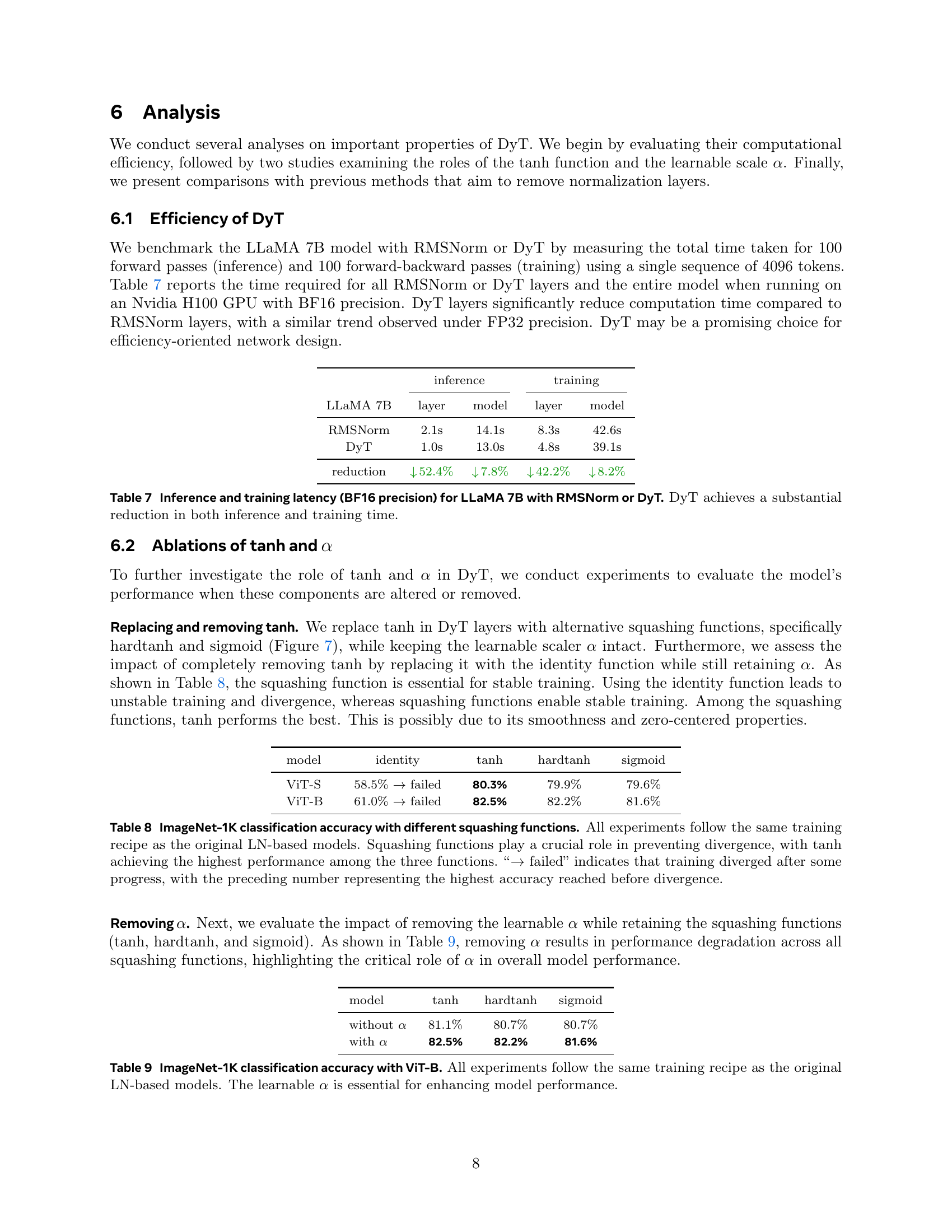
Table 7: Inference and training latency (BF16 precision) for LLaMA 7B with RMSNorm or DyT. DyT achieves a substantial reduction in both inference and training time.
| model | identity | tanh | hardtanh | sigmoid |
|---|---|---|---|---|
| ViT-S | 58.5% failed | 80.3% | 79.9% | 79.6% |
| ViT-B | 61.0% failed | 82.5% | 82.2% | 81.6% |
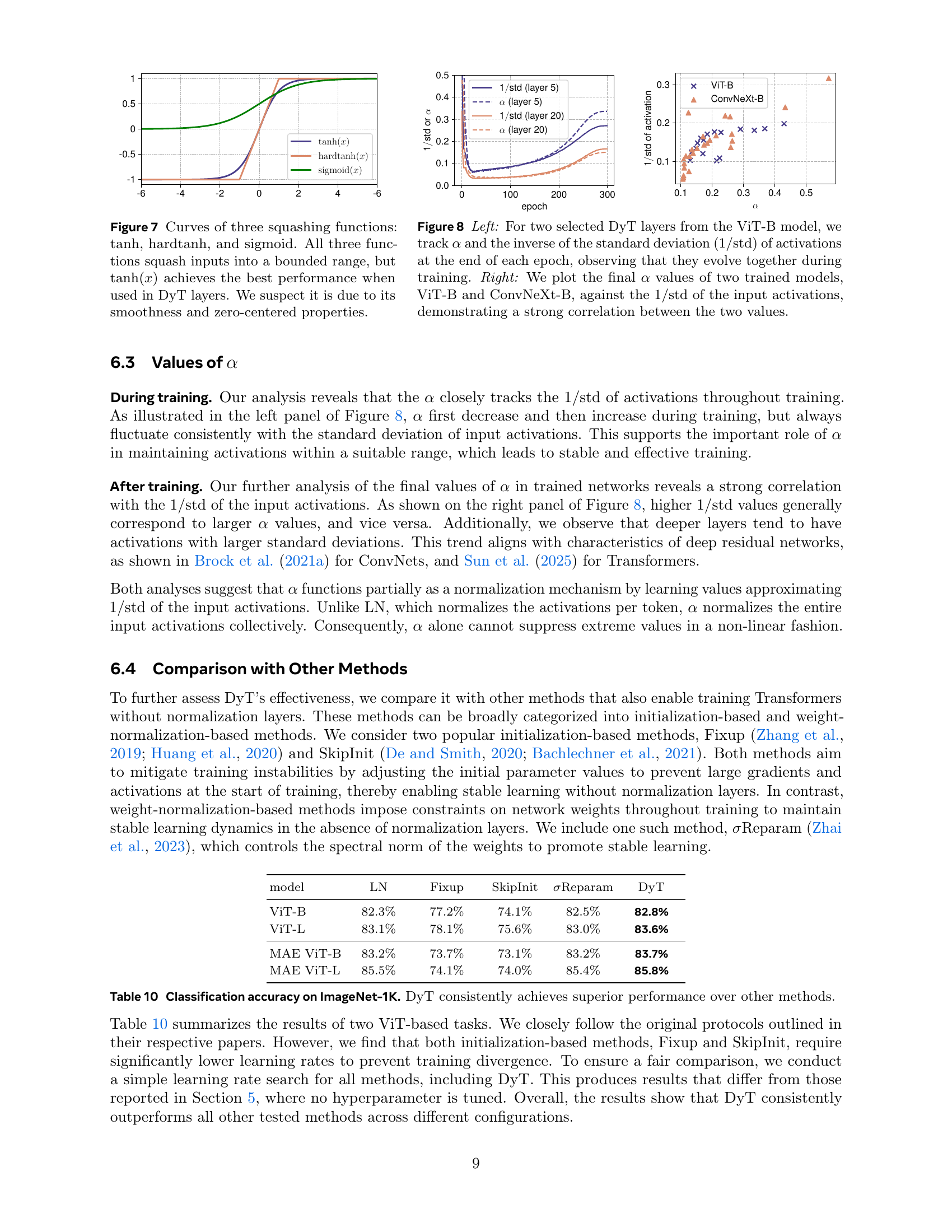
🔼 This table presents the ImageNet-1K classification accuracy results for a Vision Transformer model (ViT) using various activation functions in place of the tanh function within the DyT layer. The goal is to analyze the impact of different squashing functions on model training stability and performance. The results show that employing squashing functions is crucial for stable model training, preventing divergence, and that the tanh function yields the best performance among the tested functions (tanh, hardtanh, sigmoid). The table also highlights that the absence of a squashing function leads to training instability and divergence.
read the caption
Table 8: ImageNet-1K classification accuracy with different squashing functions. All experiments follow the same training recipe as the original LN-based models. Squashing functions play a crucial role in preventing divergence, with tanh achieving the highest performance among the three functions. “→→\rightarrow→ failed” indicates that training diverged after some progress, with the preceding number representing the highest accuracy reached before divergence.
| model | tanh | hardtanh | sigmoid |
|---|---|---|---|
| without | 81.1% | 80.7% | 80.7% |
| with | 82.5% | 82.2% | 81.6% |
🔼 This table presents the ImageNet-1K classification accuracy results for Vision Transformer (ViT-B) models. The experiments compare the performance of ViT-B models with and without the learnable scaling parameter (α) in the Dynamic Tanh (DyT) layer, while keeping other aspects of the training process consistent with the original Layer Normalization (LN) based models. The results demonstrate the importance of the learnable parameter (α) for achieving high performance in the models using DyT.
read the caption
Table 9: ImageNet-1K classification accuracy with ViT-B. All experiments follow the same training recipe as the original LN-based models. The learnable α𝛼\alphaitalic_α is essential for enhancing model performance.
| model | LN | Fixup | SkipInit | Reparam | DyT |
|---|---|---|---|---|---|
| ViT-B | 82.3% | 77.2% | 74.1% | 82.5% | 82.8% |
| ViT-L | 83.1% | 78.1% | 75.6% | 83.0% | 83.6% |
| MAE ViT-B | 83.2% | 73.7% | 73.1% | 83.2% | 83.7% |
| MAE ViT-L | 85.5% | 74.1% | 74.0% | 85.4% | 85.8% |
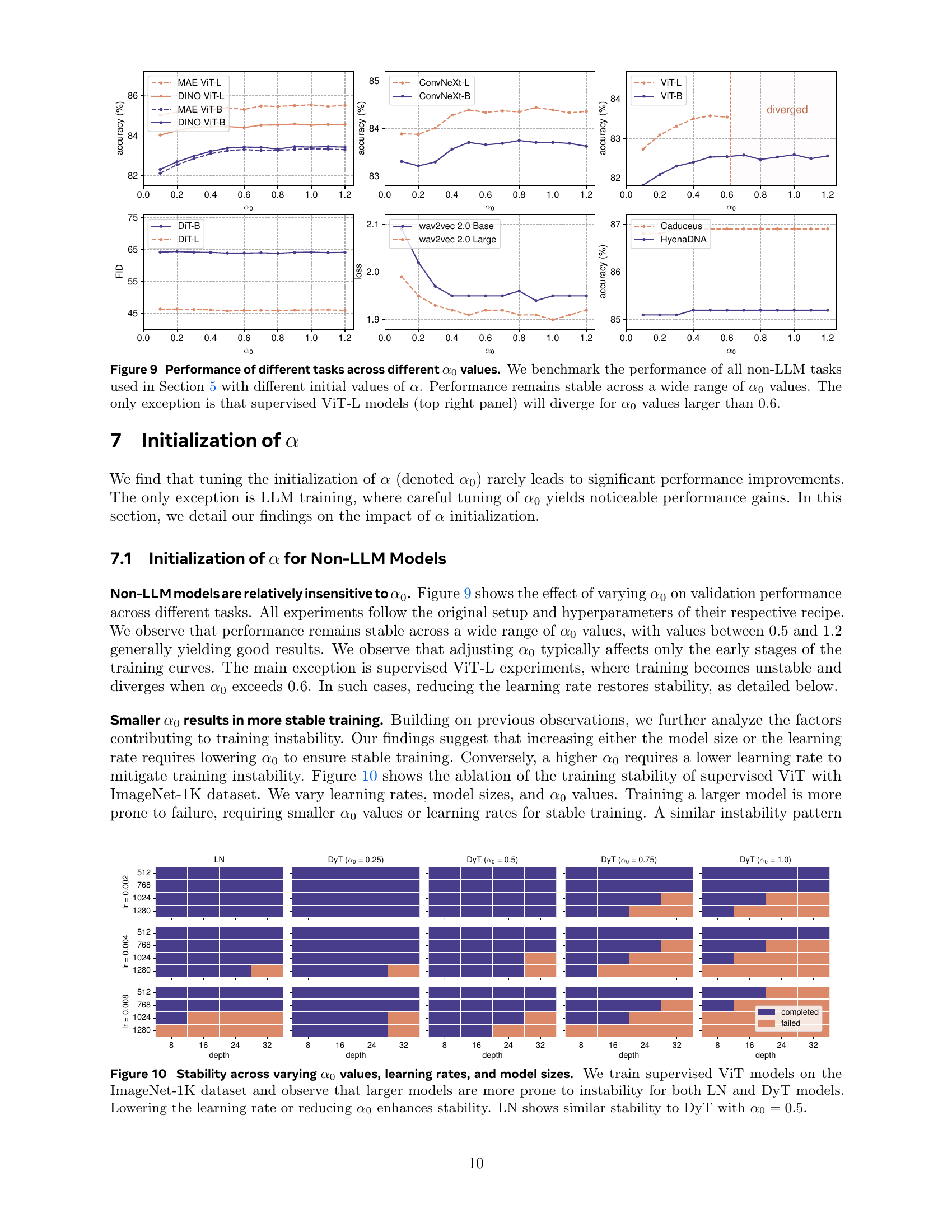
🔼 Table 10 presents a comparison of classification accuracy on the ImageNet-1K dataset across several methods for training vision transformers without normalization layers. The methods compared include DyT (Dynamic Tanh, the method proposed in the paper), Fixup, SkipInit, and Reparam. These alternative training methods are compared against the baseline approach of using Layer Normalization (LN). The results demonstrate that DyT consistently outperforms the other methods in achieving higher classification accuracy on the benchmark dataset.
read the caption
Table 10: Classification accuracy on ImageNet-1K. DyT consistently achieves superior performance over other methods.
| model | width | depth | optimal |
|---|---|---|---|
| (attention/other) | |||
| LLaMA 7B | 4096 | 32 | 0.8/0.2 |
| LLaMA 13B | 5120 | 40 | 0.6/0.15 |
| LLaMA 34B | 8196 | 48 | 0.2/0.05 |
| LLaMA 70B | 8196 | 80 | 0.2/0.05 |
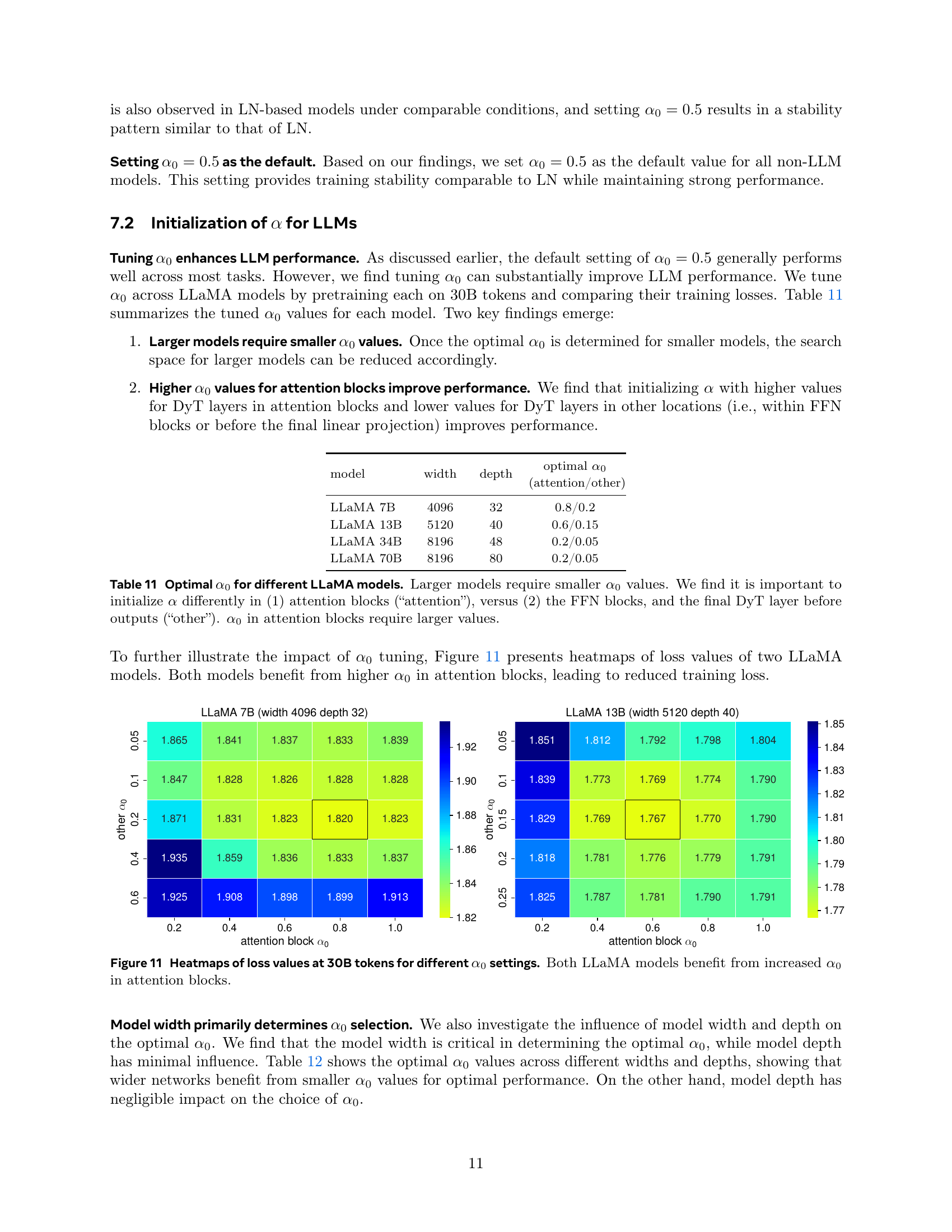
🔼 This table shows the optimal initial values for the scaling parameter α (alpha) in the Dynamic Tanh (DyT) layer for different sizes of the LLaMA language model. It reveals that larger models require smaller initial α values. Importantly, it also demonstrates that it’s beneficial to initialize α differently for the DyT layers within the attention blocks compared to the feed-forward networks (FFN) blocks and the final DyT layer before the output. Specifically, the attention blocks require significantly higher initial α values than other parts of the network.
read the caption
Table 11: Optimal α0subscript𝛼0\alpha_{0}italic_α start_POSTSUBSCRIPT 0 end_POSTSUBSCRIPT for different LLaMA models. Larger models require smaller α0subscript𝛼0\alpha_{0}italic_α start_POSTSUBSCRIPT 0 end_POSTSUBSCRIPT values. We find it is important to initialize α𝛼\alphaitalic_α differently in (1) attention blocks (“attention”), versus (2) the FFN blocks, and the final DyT layer before outputs (“other”). α0subscript𝛼0\alpha_{0}italic_α start_POSTSUBSCRIPT 0 end_POSTSUBSCRIPT in attention blocks require larger values.
| width / depth | 8 | 16 | 32 | 64 |
|---|---|---|---|---|
| 1024 | 1.0/1.0 | 1.0/1.0 | 1.0/1.0 | 1.0/1.0 |
| 2048 | 1.0/0.5 | 1.0/0.5 | 1.0/0.5 | 1.0/0.5 |
| 4096 | 0.8/0.2 | 0.8/0.2 | 0.8/0.2 | 0.8/0.2 |
| 8192 | 0.2/0.05 | 0.2/0.05 | 0.2/0.05 | 0.2/0.05 |
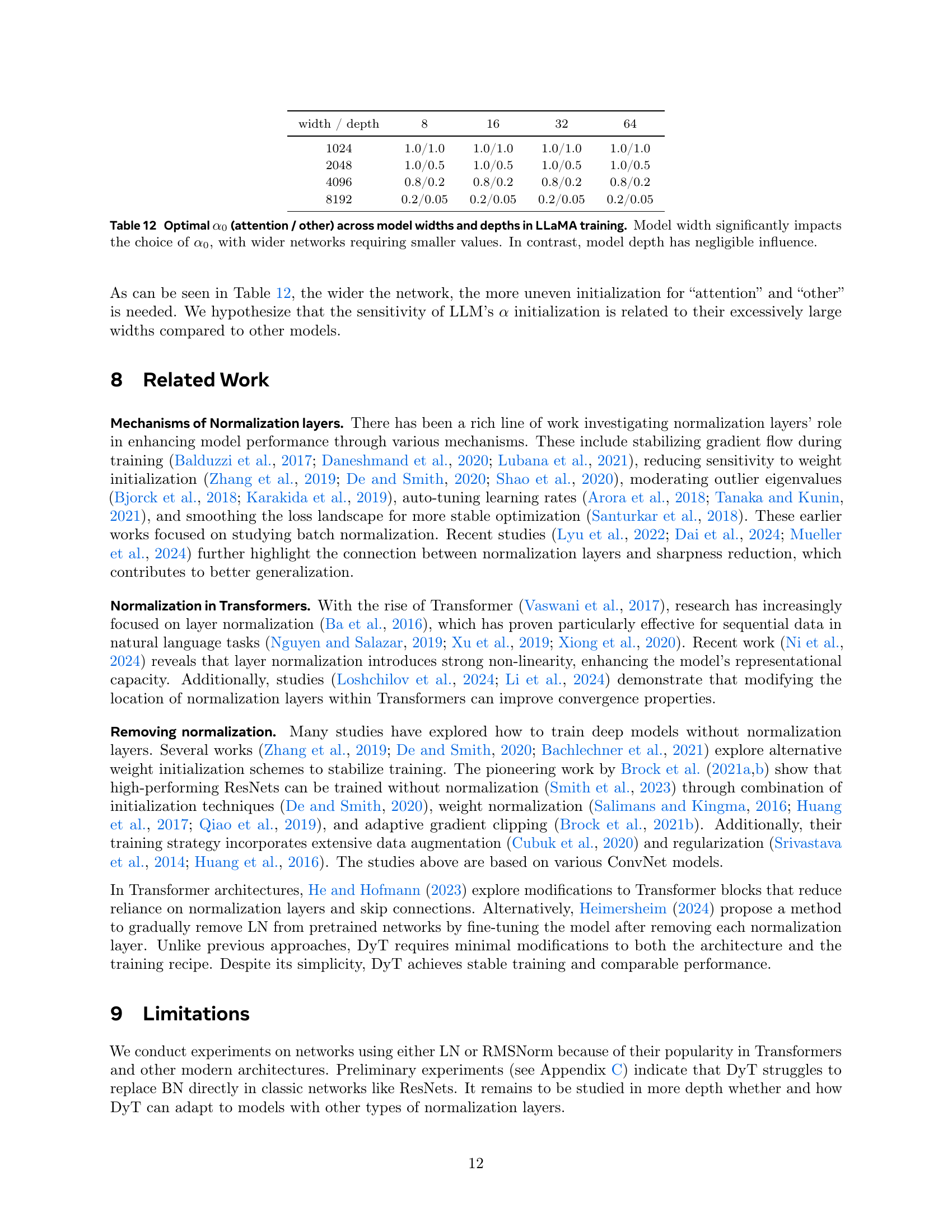
🔼 This table presents the optimal initial values for the scaling parameter α0 (alpha-zero) used in the Dynamic Tanh (DyT) layer within the LLaMA large language models. The optimal α0 values are shown for different model widths and depths, broken down into two categories: one for α0 values within attention blocks and another for α0 values elsewhere in the model. The results demonstrate a strong correlation between model width and the optimal α0: wider models necessitate smaller α0 values. Model depth, conversely, has little effect on α0 selection.
read the caption
Table 12: Optimal α0subscript𝛼0\alpha_{0}italic_α start_POSTSUBSCRIPT 0 end_POSTSUBSCRIPT (attention / other) across model widths and depths in LLaMA training. Model width significantly impacts the choice of α0subscript𝛼0\alpha_{0}italic_α start_POSTSUBSCRIPT 0 end_POSTSUBSCRIPT, with wider networks requiring smaller values. In contrast, model depth has negligible influence.
| model | LN (original) | DyT (original) | LN (tuned) | DyT (tuned) |
|---|---|---|---|---|
| ViT-B | 82.3% (4e-3) | 82.5% (4e-3) | - | 82.8% (6e-3) |
| ViT-L | 83.1% (4e-3) | 83.6% (4e-3) | - | - |
| ConvNeXt-B | 83.7% (4e-3) | 83.7% (4e-3) | - | - |
| ConvNeXt-L | 84.3% (4e-3) | 84.4% (4e-3) | - | - |
| MAE ViT-B | 83.2% (2.4e-3) | 83.2% (2.4e-3) | - | 83.7% (3.2e-3) |
| MAE ViT-L | 85.5% (2.4e-3) | 85.4% (2.4e-3) | - | 85.8% (3.2e-3) |
| DINO ViT-B (patch size 16) | 83.2% (7.5e-4) | 83.4% (7.5e-4) | 83.3% (1e-3) | - |
| DINO ViT-B (patch size 8) | 84.1% (5e-4) | 84.5% (5e-4) | - | - |
| DiT-B | 64.9 (4e-4) | 63.9 (4e-4) | - | - |
| DiT-L | 45.9 (4e-4) | 45.7 (4e-4) | - | - |
| DiT-XL | 19.9 (4e-4) | 20.8 (4e-4) | - | - |
| wav2vec 2.0 Base | 1.95 (5e-4) | 1.95 (5e-4) | - | 1.94 (6e-4) |
| wav2vec 2.0 Large | 1.92 (3e-4) | 1.91 (3e-4) | - | - |
| HyenaDNA | 85.2% (6e-4) | 85.2% (6e-4) | - | - |
| Caduceus | 86.9% (8e-3) | 86.9% (8e-3) | - | - |
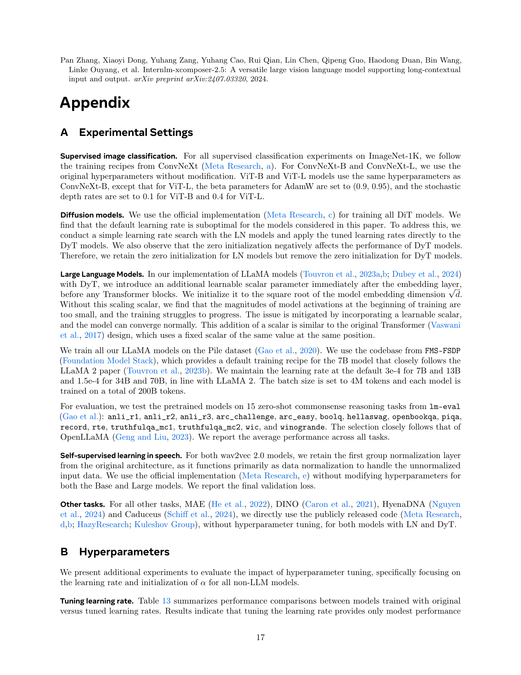
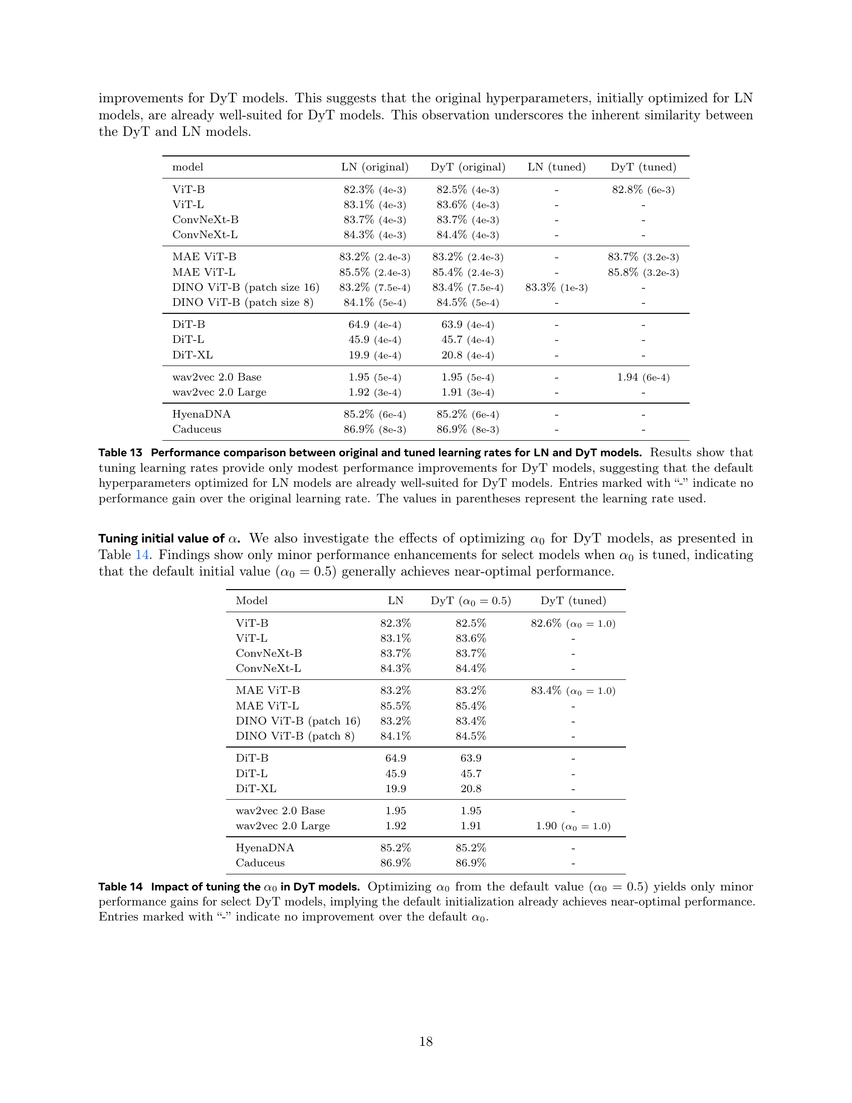
🔼 This table compares the performance of models using Layer Normalization (LN) and Dynamic Tanh (DyT) with both original and tuned learning rates on ImageNet-1K. It shows that tuning the learning rate leads to only minor improvements in DyT models, suggesting the original hyperparameters (designed for LN) are already suitable for DyT. The ‘-’ indicates instances where tuning didn’t improve performance over the original learning rate. Parenthetical values show the learning rates used.
read the caption
Table 13: Performance comparison between original and tuned learning rates for LN and DyT models. Results show that tuning learning rates provide only modest performance improvements for DyT models, suggesting that the default hyperparameters optimized for LN models are already well-suited for DyT models. Entries marked with “-” indicate no performance gain over the original learning rate. The values in parentheses represent the learning rate used.
| Model | LN | DyT () | DyT (tuned) |
|---|---|---|---|
| ViT-B | 82.3% | 82.5% | 82.6% () |
| ViT-L | 83.1% | 83.6% | - |
| ConvNeXt-B | 83.7% | 83.7% | - |
| ConvNeXt-L | 84.3% | 84.4% | - |
| MAE ViT-B | 83.2% | 83.2% | 83.4% () |
| MAE ViT-L | 85.5% | 85.4% | - |
| DINO ViT-B (patch 16) | 83.2% | 83.4% | - |
| DINO ViT-B (patch 8) | 84.1% | 84.5% | - |
| DiT-B | 64.9 | 63.9 | - |
| DiT-L | 45.9 | 45.7 | - |
| DiT-XL | 19.9 | 20.8 | - |
| wav2vec 2.0 Base | 1.95 | 1.95 | - |
| wav2vec 2.0 Large | 1.92 | 1.91 | 1.90 () |
| HyenaDNA | 85.2% | 85.2% | - |
| Caduceus | 86.9% | 86.9% | - |
🔼 Table 14 investigates the impact of modifying the initial value of the scaling parameter (α₀) within the Dynamic Tanh (DyT) layer on model performance. The experiment tunes α₀ for various model architectures and tasks, comparing the results against the default value of α₀=0.5. The findings suggest that the default initialization already yields near-optimal performance in most cases, with only minor improvements observed upon tuning α₀ for specific models. The table shows the performance differences between the baseline using the default α₀ and a model with a tuned α₀ value. A ‘-’ in the table indicates no performance improvement from tuning.
read the caption
Table 14: Impact of tuning the α0subscript𝛼0\alpha_{0}italic_α start_POSTSUBSCRIPT 0 end_POSTSUBSCRIPT in DyT models. Optimizing α0subscript𝛼0\alpha_{0}italic_α start_POSTSUBSCRIPT 0 end_POSTSUBSCRIPT from the default value (α0=0.5subscript𝛼00.5\alpha_{0}=0.5italic_α start_POSTSUBSCRIPT 0 end_POSTSUBSCRIPT = 0.5) yields only minor performance gains for select DyT models, implying the default initialization already achieves near-optimal performance. Entries marked with “-” indicate no improvement over the default α0subscript𝛼0\alpha_{0}italic_α start_POSTSUBSCRIPT 0 end_POSTSUBSCRIPT.
| model | BN | DyT |
|---|---|---|
| ResNet-50 | 76.2% | 68.9% |
| VGG19 | 72.7% | 71.0% |
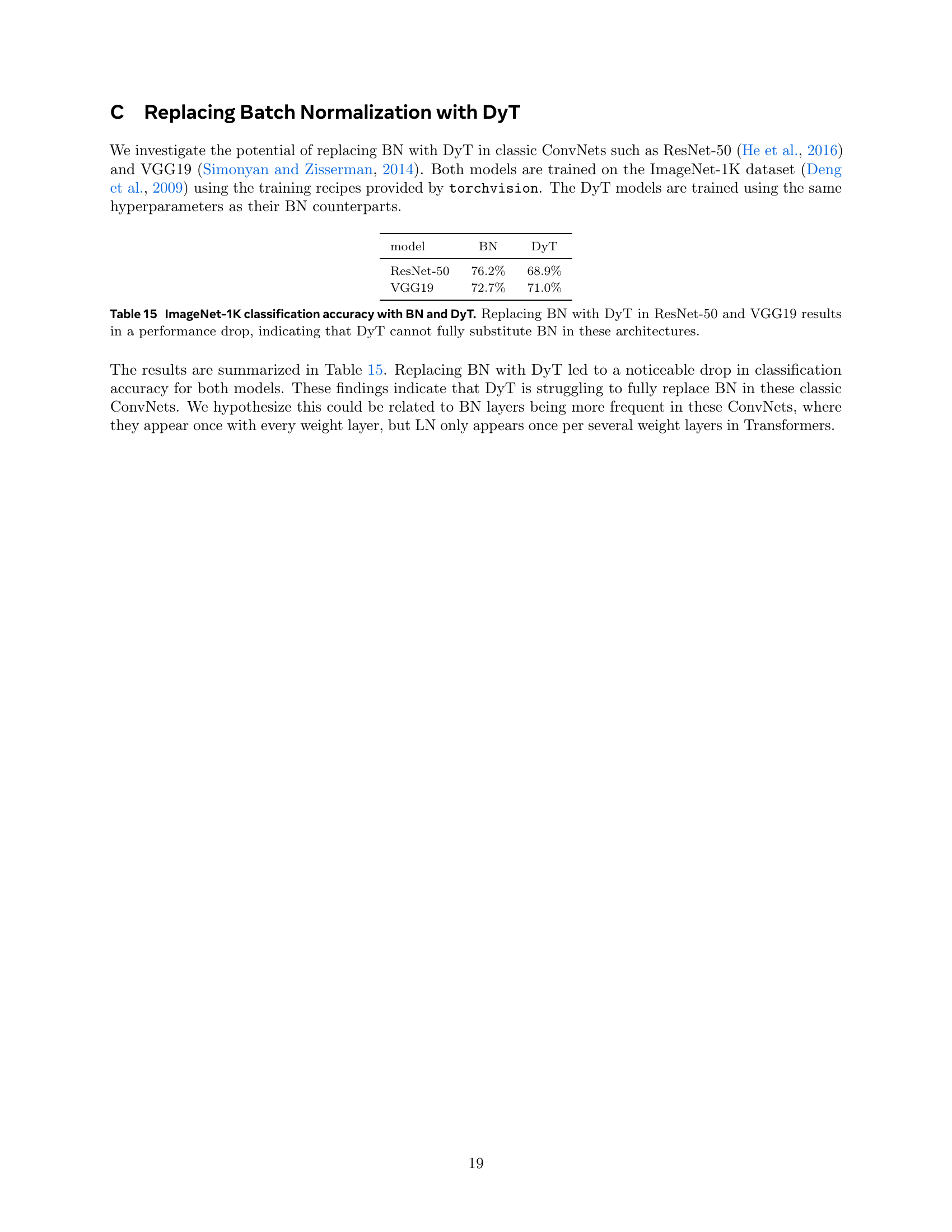
🔼 This table presents the ImageNet-1K classification accuracy results for ResNet-50 and VGG19 models, comparing the performance when using Batch Normalization (BN) against using Dynamic Tanh (DyT) as a replacement. The results show a significant performance drop when BN is replaced with DyT in both the ResNet-50 and VGG19 architectures, suggesting that DyT may not be a suitable replacement for BN in classic convolutional neural networks.
read the caption
Table 15: ImageNet-1K classification accuracy with BN and DyT. Replacing BN with DyT in ResNet-50 and VGG19 results in a performance drop, indicating that DyT cannot fully substitute BN in these architectures.
Full paper#