TL;DR#
Kolmogorov-Arnold Networks(KANs) show promise in machine learning. However, their use in vision tasks remains uncertain. Existing methods deploy KANs by substituting MLPs in vision Transformers (ViTs), prompting an investigation into their effectiveness. Initial results reveal KANs’ struggles to surpass simpler MLPs in vision, yet properly designed KANs could improve performance. Current designs lack a learnable multihead attention module, vital for Transformers, prompting the question: Can learnable multi-head self-attention enhance (vision) Transformers?
This paper introduces a general learnable Kolmogorov-Arnold Attention (KArAt) for vanilla ViTs, operating on any basis. Addressing high computing and memory costs, a modular version, Fourier-KArAt, is proposed. Experiments show Fourier-KArAt either outperforms ViT counterparts or matches their performance on standard image datasets. Through loss landscape, weight distribution, attention visualization, and spectral behavior analyses, the architectures’ performance and generalization are dissected, offering a benchmark and insights into KANs in advanced architectures.
Key Takeaways#
Why does it matter?#
This paper pioneers learnable attention in vision transformers, offering insights into architecture performance and encouraging exploration of KANs with advanced architectures. It opens avenues for innovative attention mechanisms & future LMM applications, challenging existing paradigms.
Visual Insights#

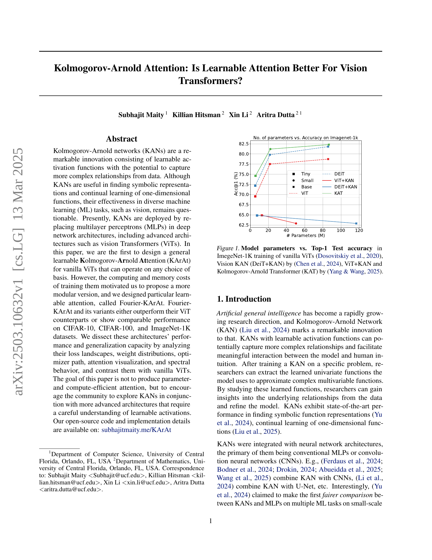
🔼 This figure compares the performance of different vision transformer models on the ImageNet-1K dataset. The x-axis represents the number of model parameters (in millions), while the y-axis shows the Top-1 test accuracy. The plot includes results for vanilla Vision Transformers (ViTs) of varying sizes (Tiny, Small, Base), Vision KAN (DeiT+KAN) which replaces MLP layers in DeiT with KANs, ViT+KAN that replaces MLP layers in ViTs with KANs, and the Kolmogorov-Arnold Transformer (KAT) which uses a refined group-KAN strategy. The figure illustrates the relationship between model complexity and accuracy, allowing for a comparison of different approaches to incorporating Kolmogorov-Arnold networks into vision transformers.
read the caption
Figure 1: Model parameters vs. Top-1 Test accuracy in ImegeNet-1K training of vanilla ViTs (Dosovitskiy et al., 2020), Vision KAN (DeiT+KAN) by (Chen et al., 2024), ViT+KAN and Kolmogorov-Arnold Transformer (KAT) by (Yang & Wang, 2025).
| Model | CIFAR-10 | CIFAR-100 | Imagenet-1K | Parameters | |||
|---|---|---|---|---|---|---|---|
| Acc.@1 | Acc.@5 | Acc.@1 | Acc.@5 | Acc.@1 | Acc.@5 | ||
| ViT-Base | 83.45 | 99.19 | 58.07 | 83.70 | 72.90 | 90.56 | 85.81M |
| + | 81.81 (1.97%) | 99.01 | 55.92(3.70%) | 82.04 | 68.03(6.68%) | 86.41 | 87.51M (1.98% ) |
| + | 80.75(3.24%) | 98.76 | 57.36 (1.22% ) | 82.89 | 68.83 (5.58%) | 87.69 | 85.95M (0.16% ) |
| ViT-Small | 81.08 | 99.02 | 53.47 | 82.52 | 70.50 | 89.34 | 22.05M |
| + | 79.78 (1.60%) | 98.70 | 54.11 (1.20%) | 81.02 | 67.77 (3.87%) | 87.51 | 23.58M (6.94%) |
| + | 79.52(1.92%) | 98.85 | 53.86(0.73%) | 81.45 | 67.76(3.89%) | 87.60 | 22.18M (0.56%) |
| ViT-Tiny | 72.76 | 98.14 | 43.53 | 75.00 | 59.15 | 82.07 | 5.53M |
| + | 76.69(5.40%) | 98.57 | 46.29(6.34%) | 77.02 | 59.11 (0.07%) | 82.01 | 6.29M (13.74%) |
| + | 75.56 (3.85%) | 98.48 | 46.75(7.40%) | 76.81 | 57.97(1.99%) | 81.03 | 5.59M (1.08%) |
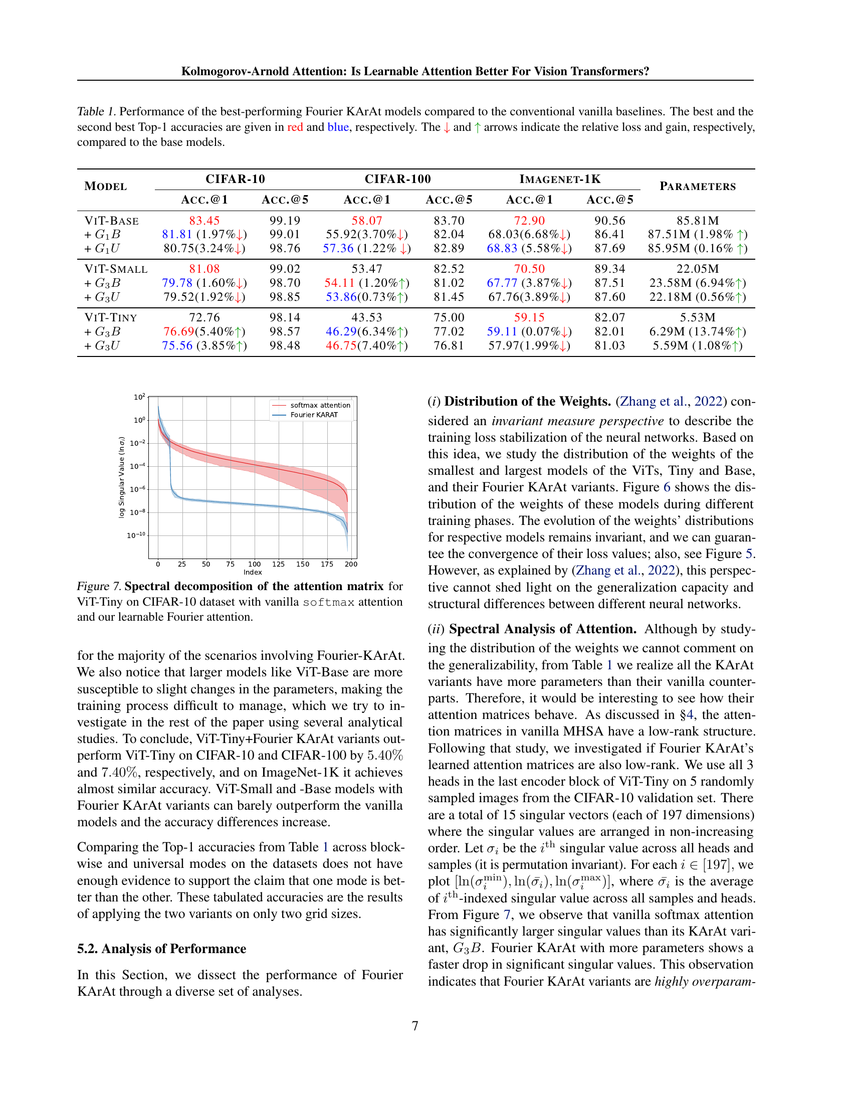
🔼 This table presents a comparison of the performance of several vision transformer models on three benchmark datasets (CIFAR-10, CIFAR-100, and ImageNet-1K). The models include various vanilla Vision Transformers (ViT-Tiny, ViT-Small, ViT-Base) and their counterparts enhanced with the Fourier Kolmogorov-Arnold Attention (Fourier KArAt) mechanism. The table shows the top-1 and top-5 accuracy results for each model on each dataset. The best and second-best Top-1 accuracy results for each vanilla ViT are highlighted in red and blue, respectively, to easily identify the improvement or degradation provided by the Fourier KArAt. Percentage increases or decreases in accuracy compared to the vanilla ViTs are also provided using arrows to indicate gains (↑↑) or losses (↓↓). The number of parameters for each model is also listed to provide context for performance differences.
read the caption
Table 1: Performance of the best-performing Fourier KArAt models compared to the conventional vanilla baselines. The best and the second best Top-1 accuracies are given in red and blue, respectively. The ↓↓\downarrow↓ and ↑↑\uparrow↑ arrows indicate the relative loss and gain, respectively, compared to the base models.
In-depth insights#
KANs: Vision Lens#
While KANs have shown promise, their efficacy in vision tasks remains a question. The research explores using KANs within Vision Transformers (ViTs), a more advanced architecture. The paper introduces a learnable Kolmogorov-Arnold Attention (KArAt) mechanism, demonstrating its potential for capturing intricate relationships in image data. The core idea revolves around replacing traditional components in ViTs with KANs, specifically the multi-layer perceptrons (MLPs), to enhance feature extraction and representation learning. The investigation delves into whether these learnable activations offered by KANs can genuinely improve the performance and generalization of ViTs compared to standard attention mechanisms. Furthermore, a modular version, Fourier-KArAt is introduced that showcases better performance in terms of computational efficiency and memory usage.
KArAt:ViT Module#
The KArAt:ViT module represents an innovative approach to integrating Kolmogorov-Arnold Networks (KANs) into Vision Transformers (ViTs). This integration aims to leverage the learnable activation functions of KANs to enhance the feature extraction and representation learning capabilities of ViTs. By replacing traditional components, such as MLPs, with KANs, the module potentially allows the network to capture more complex relationships within the data. This module could lead to improved performance in image classification tasks due to the enhanced representational capacity offered by KANs. However, the complexity of KANs may also introduce challenges, such as increased computational cost and potential overfitting, which requires careful design and optimization.
Low-Rank KArAt#
The paper addresses the computational cost of Kolmogorov-Arnold Networks (KANs) in vision transformers, specifically focusing on attention mechanisms. Addressing the bottleneck of high computational costs, they propose exploiting the low-rank structure inherent in attention matrices, drawing parallels to observations in other deep networks. Aiming to reduce computational complexity, they introduce a reduced-size operator with learnable activation in a lower-dimensional subspace. By projecting attention row vectors, significantly diminishes computational overhead. Then, uses a learnable weight matrix to project them back to original dimension. They found that this approach also helps to increase the computational efficiency, offering a practical way to integrate KANs without prohibitive costs.
B-Splines’ Drawback#
The paper identifies limitations of using B-Splines as basis functions within Kolmogorov-Arnold Networks (KANs), specifically mentioning their localized nature which hinders leveraging standard CUDA functions for efficient GPU acceleration, unlike global basis functions like Fourier transforms. This localization results in slower execution speeds, complicating the GPU implementation process and making it non-scalable. Furthermore, experiments reveal that B-spline KANs demonstrate poor generalizability on medium-scale datasets such as CIFAR-10 and CIFAR-100, despite achieving high accuracies on smaller datasets such as MNIST and Fashion-MNIST. This highlights the importance of basis function selection and emphasizes the need for alternatives with better computational characteristics and generalizability.
MHSA’s Data Role#
MHSA (Multi-Head Self-Attention)’s data role is paramount in vision transformers. MHSA excels at capturing intricate relationships within image data. Each attention head learns different aspects of these relationships, enabling the network to focus on diverse patterns and contextual dependencies. This is achieved by calculating attention weights based on the similarity between query, key, and value embeddings, effectively weighing the importance of different image regions for each head. These weights are then used to aggregate information from the value embeddings, highlighting the most relevant features for each head. This process allows the transformer to model complex dependencies and interactions within the image data, resulting in robust and accurate representations essential for tasks like image classification, object detection, and segmentation. The architecture’s capability to learn diverse patterns and interdependencies leads to a more robust representation for downstream vision tasks.
More visual insights#
More on figures

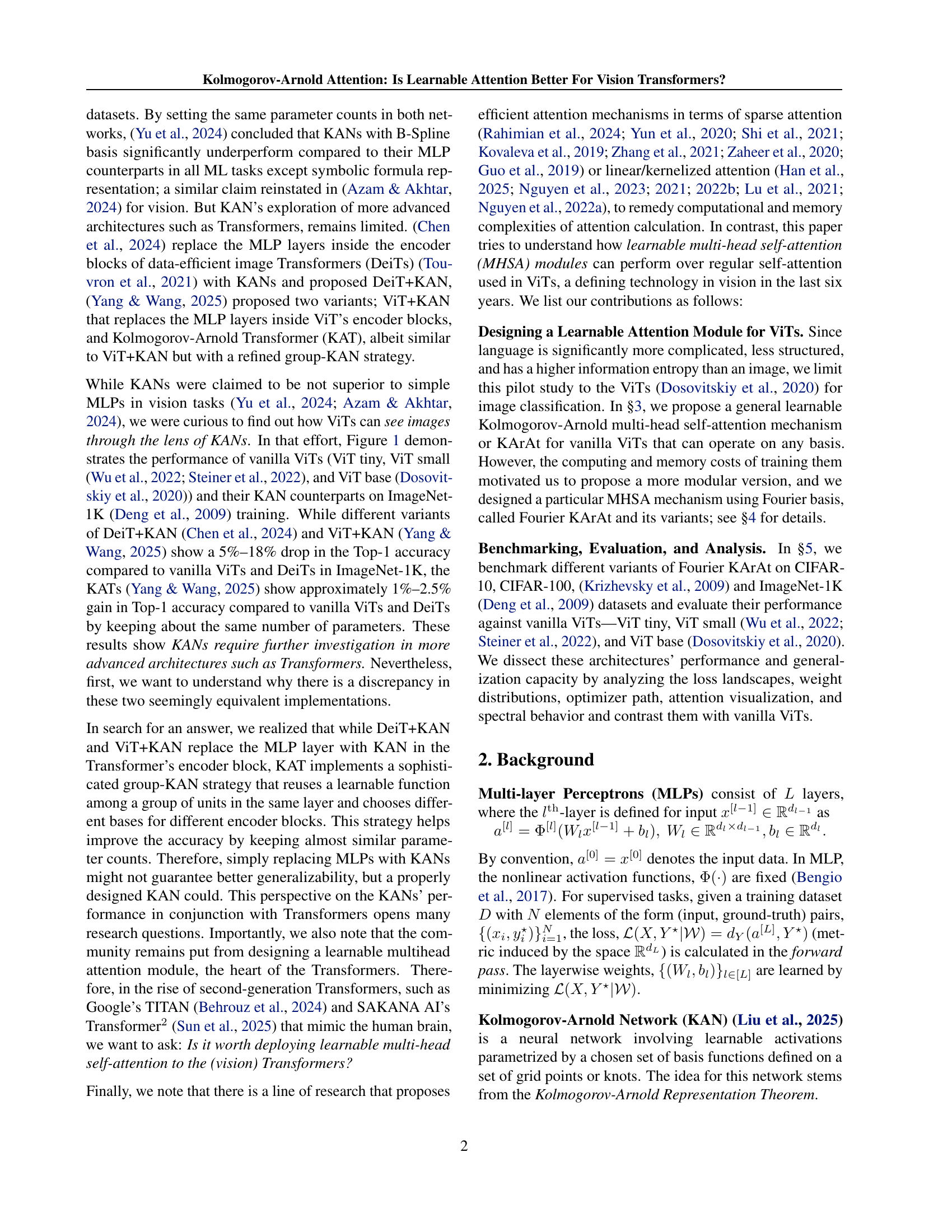
🔼 Figure 2 illustrates the architecture of the proposed Kolmogorov-Arnold Attention (KArAt). (a) shows the standard softmax self-attention mechanism where the attention matrix is computed using the scaled dot-product of query, key, and value matrices. (b) replaces the softmax function with a learnable function, which is the core idea of KArAt. (c) depicts the ideal KArAt, where a large N x N learnable operator matrix acts directly on the attention matrix. However, due to computational limitations, (d) presents the practical implementation of KArAt using a smaller N x r learnable operator followed by a linear projection. This reduced architecture makes training feasible while still capturing the essence of learnable attention.
read the caption
Figure 2: (a) The standard softmax self-attention for ithsuperscript𝑖thi^{\rm th}italic_i start_POSTSUPERSCRIPT roman_th end_POSTSUPERSCRIPT head in the jthsuperscript𝑗thj^{\rm th}italic_j start_POSTSUPERSCRIPT roman_th end_POSTSUPERSCRIPT encoder block. (b) The Kolmogorov-Arnold Attention (KArAt) replaces the softmax with a learnable function Φi,jsuperscriptΦ𝑖𝑗\Phi^{i,j}roman_Φ start_POSTSUPERSCRIPT italic_i , italic_j end_POSTSUPERSCRIPT. (c) The ideal KArAt is with an operator matrix, Φi,jsuperscriptΦ𝑖𝑗\Phi^{i,j}roman_Φ start_POSTSUPERSCRIPT italic_i , italic_j end_POSTSUPERSCRIPT with N×N𝑁𝑁N\times Nitalic_N × italic_N learnable units that act on each row of 𝒜i,jsuperscript𝒜𝑖𝑗{\cal A}^{i,j}caligraphic_A start_POSTSUPERSCRIPT italic_i , italic_j end_POSTSUPERSCRIPT. (d) While Φi,j∈ℝN×NsuperscriptΦ𝑖𝑗superscriptℝ𝑁𝑁\Phi^{i,j}\in\mathbb{R}^{N\times N}roman_Φ start_POSTSUPERSCRIPT italic_i , italic_j end_POSTSUPERSCRIPT ∈ blackboard_R start_POSTSUPERSCRIPT italic_N × italic_N end_POSTSUPERSCRIPT is impossible to implement due to computational constraints, our architecture uses an operator Φ^i,jsuperscript^Φ𝑖𝑗\widehat{\Phi}^{i,j}over^ start_ARG roman_Φ end_ARG start_POSTSUPERSCRIPT italic_i , italic_j end_POSTSUPERSCRIPT with N×r𝑁𝑟N\times ritalic_N × italic_r learnable units r≪Nmuch-less-than𝑟𝑁r\ll Nitalic_r ≪ italic_N, followed by a linear projector with learnable weights W∈ℝr×N𝑊superscriptℝ𝑟𝑁W\in\mathbb{R}^{r\times N}italic_W ∈ blackboard_R start_POSTSUPERSCRIPT italic_r × italic_N end_POSTSUPERSCRIPT.

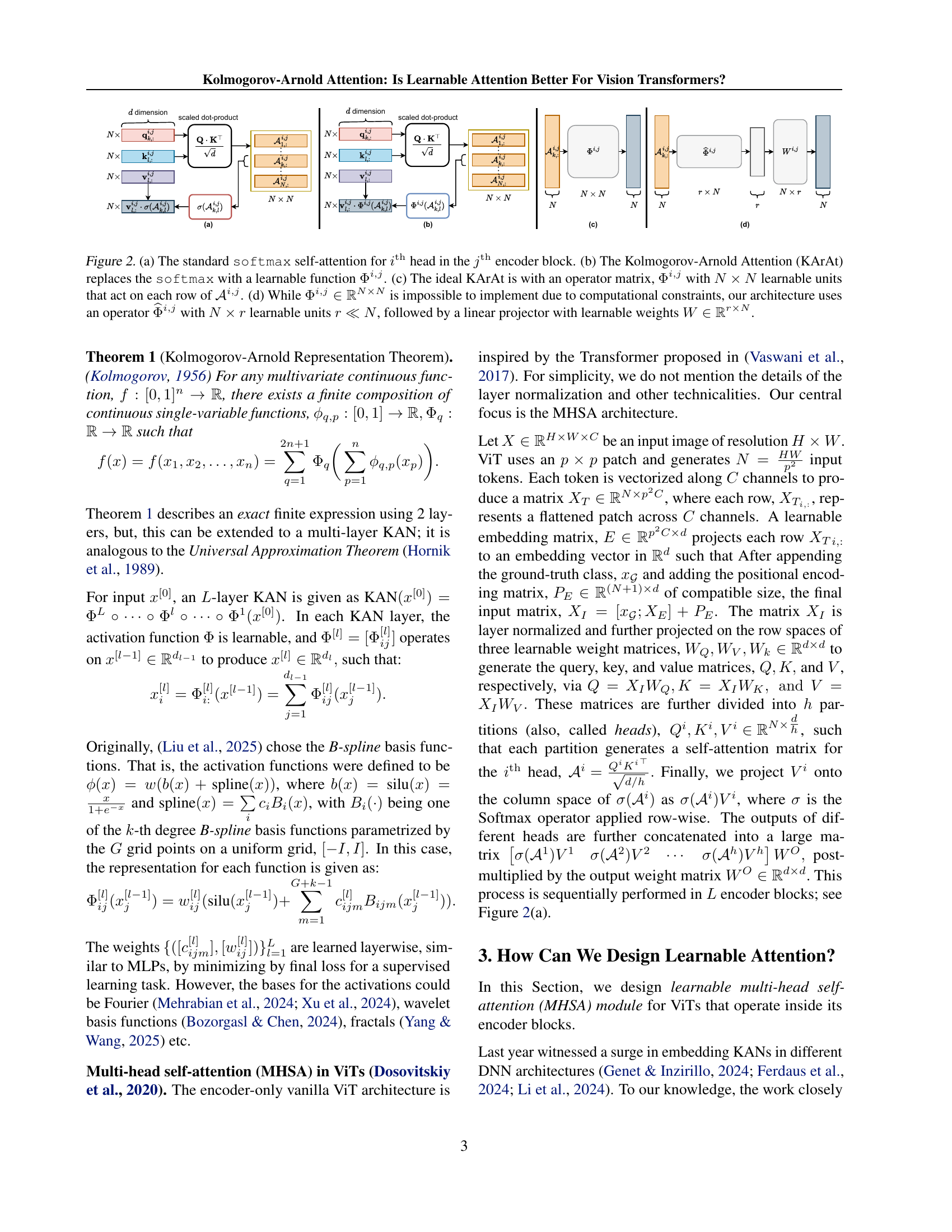
🔼 Figure 3(a) displays the spectral analysis of attention matrices in the jth encoder block’s ith head before applying the softmax function. The analysis uses all three heads in the last encoder block of a ViT-tiny model, processing five randomly selected images from the CIFAR-10 validation set. The plot shows 15 singular vectors (each with 197 dimensions), with singular values arranged in descending order.
read the caption
(a) Attention matrix 𝒜i,jsuperscript𝒜𝑖𝑗{\mathcal{A}^{i,j}}caligraphic_A start_POSTSUPERSCRIPT italic_i , italic_j end_POSTSUPERSCRIPT before softmax activation.

🔼 The figure shows a heatmap visualization of the attention matrix after applying the softmax activation function. Each row of the matrix represents a query vector, and each column represents a key vector. The values in the matrix indicate the attention weights between each query-key pair. The softmax function normalizes these weights, so that they sum to 1 for each row. The visualization helps to understand the focus of the attention mechanism on different regions of the input image.
read the caption
(b) Attention matrix σ(𝒜i,j)𝜎superscript𝒜𝑖𝑗\sigma(\mathcal{A}^{i,j})italic_σ ( caligraphic_A start_POSTSUPERSCRIPT italic_i , italic_j end_POSTSUPERSCRIPT ) after softmax activation.

🔼 This figure presents a spectral analysis of attention matrices from a Vision Transformer (ViT-tiny) model, comparing the singular value decomposition (SVD) before and after applying the softmax activation function. The analysis uses the last encoder block’s three attention heads and five randomly chosen images from the CIFAR-10 validation set. The plot displays the 15 singular vectors (one for each head across the five images), each having 197 dimensions, with singular values arranged in descending order. The results visually demonstrate that the attention matrices exhibit a low-rank structure, both before and after the softmax activation.
read the caption
Figure 3: Spectral analysis of the attention matrices before and after softmax shows that they are low-rank. For this experiment, we use all 3 heads in the last encoder block of ViT tiny on 5 randomly sampled images from the CIFAR-10 validation set. We plot all 15 singular vectors (each of 197 dimensions) where the singular values are arranged in non-increasing order.

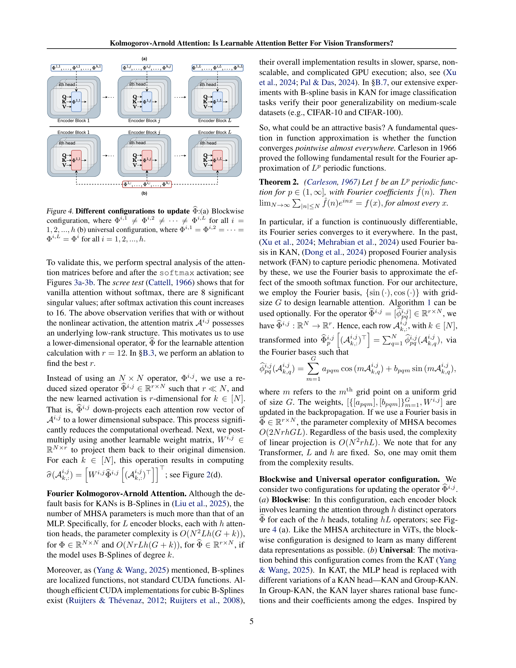
🔼 Figure 4 illustrates two different ways of updating the learnable activation function, Φ, within the multi-head self-attention mechanism of a Vision Transformer. In the (a) Blockwise configuration, a separate Φ is learned for each head (indexed by i) and each encoder block (indexed by j), allowing for greater flexibility and potential to capture diverse relationships within the data. Each head learns different patterns in different blocks. In the (b) Universal configuration, a single Φ is learned and shared across all heads and blocks, making the model more efficient but potentially less capable of adapting to complex data patterns. All heads share the same learned parameters in all blocks.
read the caption
Figure 4: Different configurations to update Φ^^Φ\widehat{\Phi}over^ start_ARG roman_Φ end_ARG:(a) Blockwise configuration, where Φi,1≠Φi,2≠⋯≠Φi,LsuperscriptΦ𝑖1superscriptΦ𝑖2⋯superscriptΦ𝑖𝐿\Phi^{i,1}\neq\Phi^{i,2}\neq\cdots\neq\Phi^{i,L}roman_Φ start_POSTSUPERSCRIPT italic_i , 1 end_POSTSUPERSCRIPT ≠ roman_Φ start_POSTSUPERSCRIPT italic_i , 2 end_POSTSUPERSCRIPT ≠ ⋯ ≠ roman_Φ start_POSTSUPERSCRIPT italic_i , italic_L end_POSTSUPERSCRIPT for all i=1,2,…,h𝑖12…ℎi=1,2,...,hitalic_i = 1 , 2 , … , italic_h (b) universal configuration, where Φi,1=Φi,2=⋯=Φi,L=ΦisuperscriptΦ𝑖1superscriptΦ𝑖2⋯superscriptΦ𝑖𝐿superscriptΦ𝑖\Phi^{i,1}=\Phi^{i,2}=\cdots=\Phi^{i,L}=\Phi^{i}roman_Φ start_POSTSUPERSCRIPT italic_i , 1 end_POSTSUPERSCRIPT = roman_Φ start_POSTSUPERSCRIPT italic_i , 2 end_POSTSUPERSCRIPT = ⋯ = roman_Φ start_POSTSUPERSCRIPT italic_i , italic_L end_POSTSUPERSCRIPT = roman_Φ start_POSTSUPERSCRIPT italic_i end_POSTSUPERSCRIPT for all i=1,2,…,h.𝑖12…ℎi=1,2,...,h.italic_i = 1 , 2 , … , italic_h .

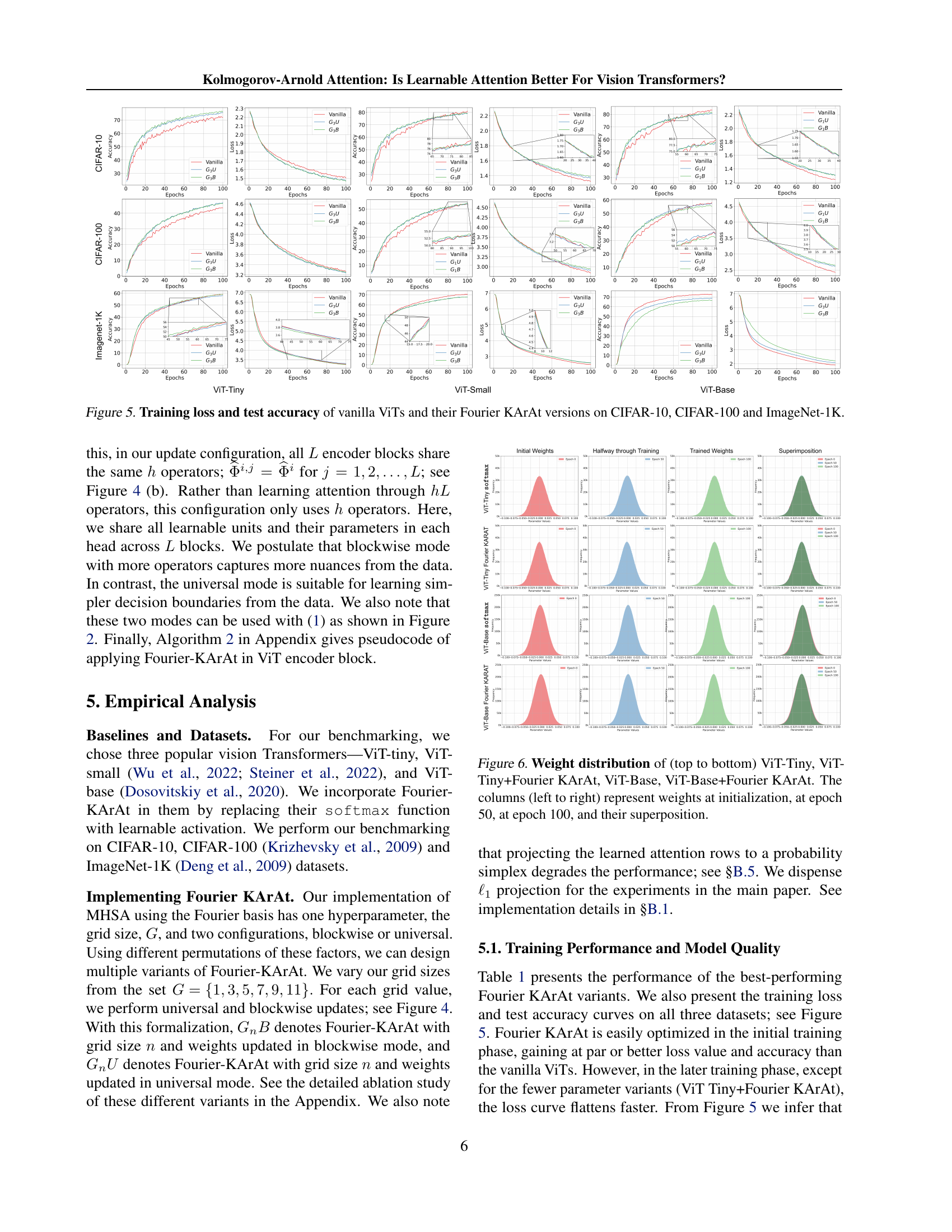
🔼 This figure displays the training loss and testing accuracy curves for standard Vision Transformers (ViTs) and modified versions incorporating Fourier Kolmogorov-Arnold Attention (Fourier KArAt) across three benchmark datasets: CIFAR-10, CIFAR-100, and ImageNet-1K. Separate curves are shown for each dataset and model variant (ViT-Tiny, ViT-Small, ViT-Base with and without Fourier KArAt). The plots allow for a visual comparison of the training performance and generalization ability of the models, highlighting the differences in convergence speed and final accuracy.
read the caption
Figure 5: Training loss and test accuracy of vanilla ViTs and their Fourier KArAt versions on CIFAR-10, CIFAR-100 and ImageNet-1K.

🔼 This figure visualizes the weight distributions of four different models at various training stages. The top two rows show the weight distributions for ViT-Tiny and ViT-Tiny enhanced with Fourier KArAt. The bottom two rows illustrate the weight distributions for ViT-Base and ViT-Base enhanced with Fourier KArAt. Each row displays four columns, representing the weight distribution at initialization, after 50 epochs, after 100 epochs, and a superposition of these three. This visual representation allows for a comparison of how weight distributions evolve during training in standard Vision Transformers (ViTs) and ViTs that incorporate learnable Fourier Kolmogorov-Arnold Attention (Fourier KArAt).
read the caption
Figure 6: Weight distribution of (top to bottom) ViT-Tiny, ViT-Tiny+Fourier KArAt, ViT-Base, ViT-Base+Fourier KArAt. The columns (left to right) represent weights at initialization, at epoch 50, at epoch 100, and their superposition.

🔼 This figure displays the singular value decomposition of the attention matrices from ViT-Tiny model trained on CIFAR-10 dataset. It compares the spectral properties of attention matrices generated using the standard softmax activation function and the proposed learnable Fourier attention mechanism. The plot shows the singular values (log scale) against their index, illustrating the relative importance of different components in each attention matrix. The relative importance of the singular values reflects the low rank nature of the attention mechanism. Comparing the two shows the difference in the distributions of the singular values between the standard softmax and the learnable Fourier attention, indicating a difference in the complexity of their respective information encoding.
read the caption
Figure 7: Spectral decomposition of the attention matrix for ViT-Tiny on CIFAR-10 dataset with vanilla softmax attention and our learnable Fourier attention.

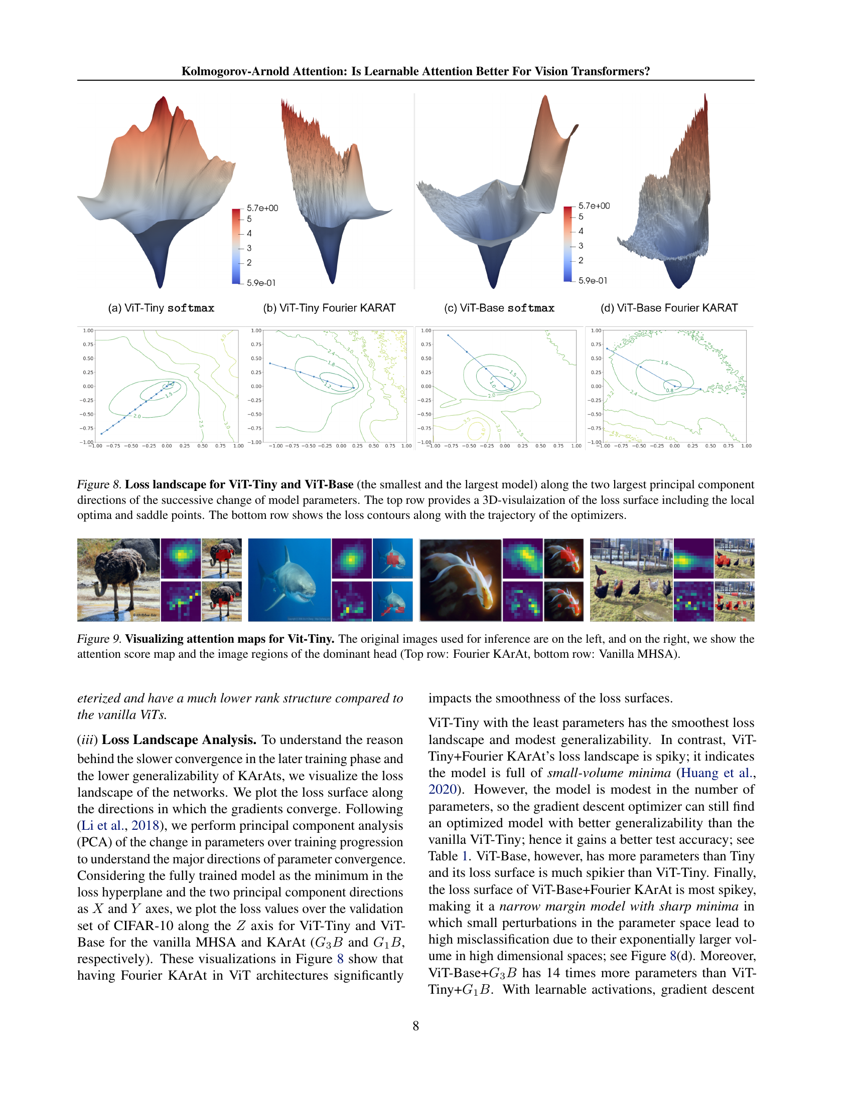
🔼 This figure visualizes the loss landscapes of ViT-Tiny and ViT-Base models, comparing the vanilla softmax attention mechanism with the Fourier KArAt variant. The top row presents 3D visualizations of the loss surfaces, highlighting local optima (minima) and saddle points. These points represent areas of the loss surface where the model’s performance is either optimal or relatively unchanging with respect to small parameter changes. The bottom row displays 2D contour plots of the loss landscapes. The paths of the optimizers during training are overlaid on these contours, illustrating the model’s journey through the loss landscape towards the minimum. By comparing the loss landscapes of the vanilla and Fourier KArAt models, the visualization offers insights into their optimization behavior and generalization capabilities.
read the caption
Figure 8: Loss landscape for ViT-Tiny and ViT-Base (the smallest and the largest model) along the two largest principal component directions of the successive change of model parameters. The top row provides a 3D-visulaization of the loss surface including the local optima and saddle points. The bottom row shows the loss contours along with the trajectory of the optimizers.
🔼 This figure visualizes attention maps for ViT-Tiny, comparing Fourier KArAt and Vanilla MHSA. The left side shows the original images used for inference. The right side displays both the attention score map (highlighting which parts of the image the model focuses on) and the corresponding image regions of the dominant head (most influential part of the attention mechanism). The top row shows results from using Fourier KArAt, while the bottom row shows results using the standard Vanilla MHSA.
read the caption
Figure 9: Visualizing attention maps for Vit-Tiny. The original images used for inference are on the left, and on the right, we show the attention score map and the image regions of the dominant head (Top row: Fourier KArAt, bottom row: Vanilla MHSA).

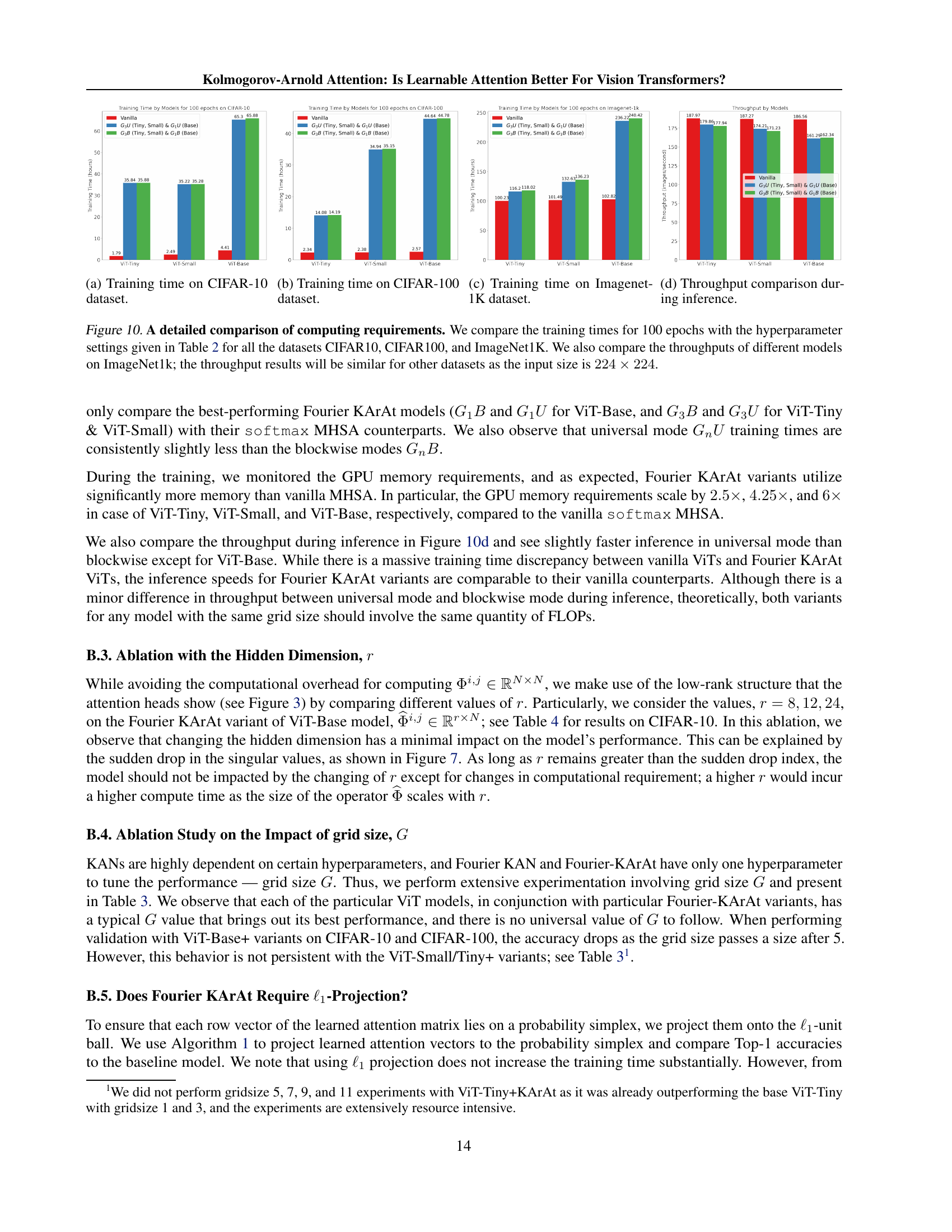
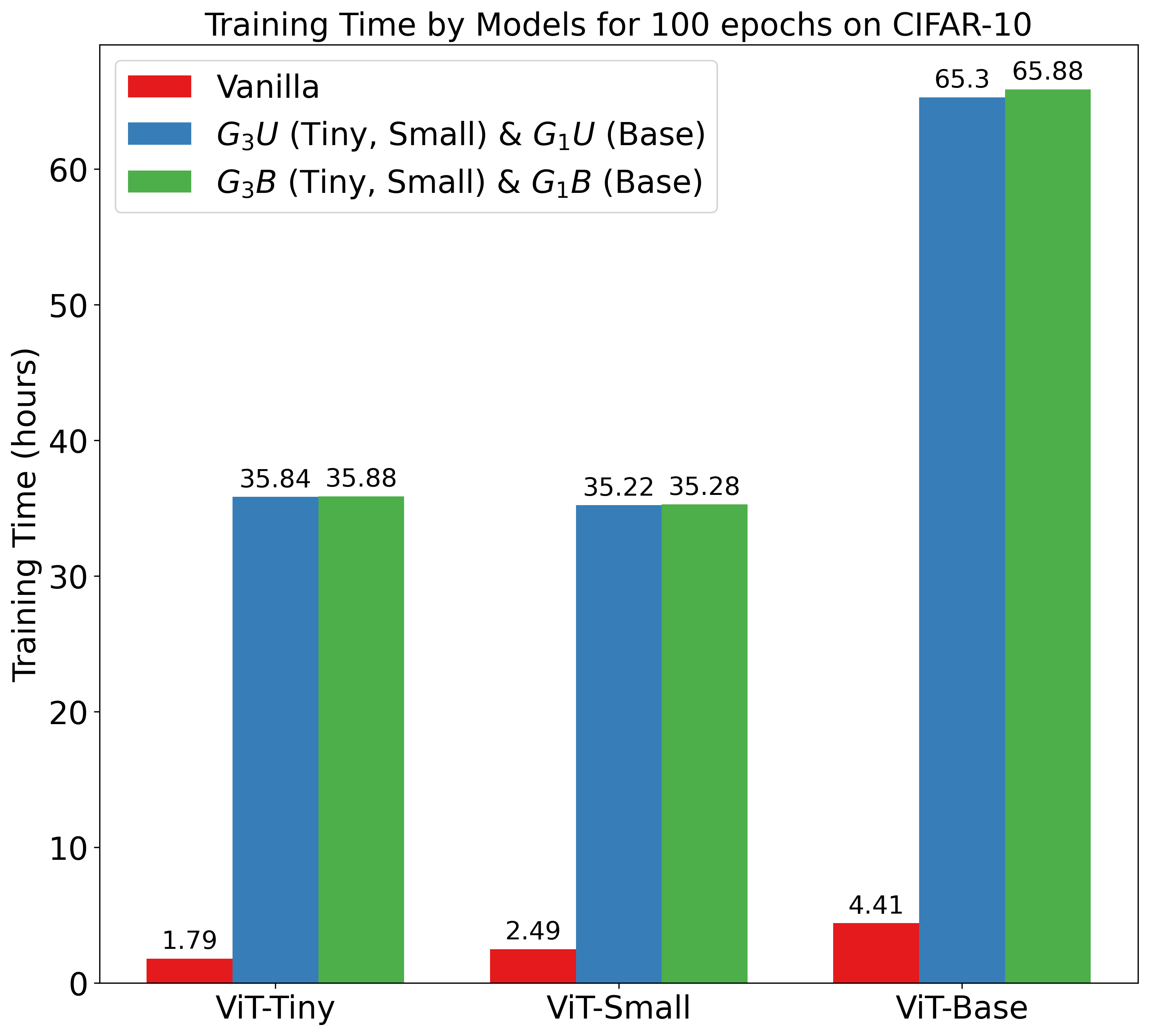
🔼 This figure displays a bar chart comparing the training times of various Vision Transformer models on the CIFAR-10 dataset. The models compared include the vanilla ViT (without learnable attention), and several variants of the Fourier KArAt model. The Fourier KArAt models are differentiated by their grid size (G) and update configuration (blockwise or universal), reflecting different settings for the learnable attention mechanism. The chart visually represents the computational cost associated with each model, allowing for easy comparison of training efficiency between the vanilla ViT and the different configurations of Fourier KArAt.
read the caption
(a) Training time on CIFAR-10 dataset.

🔼 This figure shows the training time in hours for different vision transformer models (ViT-Tiny, ViT-Small, ViT-Base) and their corresponding Fourier KArAt variants on the CIFAR-100 dataset. The training was conducted for 100 epochs using the hyperparameters listed in Table 2 of the paper. The figure compares the training times of vanilla models with their Fourier KArAt counterparts (G3U/G1U for universal configuration and G3B/G1B for blockwise configuration), showing the increase in training time introduced by the learnable attention mechanism.
read the caption
(b) Training time on CIFAR-100 dataset.

🔼 This figure shows the training time in hours for different Vision Transformer models (ViT-Tiny, ViT-Small, ViT-Base) and their corresponding Fourier KArAt versions on the ImageNet-1K dataset. The training was conducted for 100 epochs using the hyperparameters specified in Table 2 of the paper. The figure allows for a comparison of the computational cost between vanilla Vision Transformers and their Fourier KArAt counterparts across different model sizes.
read the caption
(c) Training time on Imagenet-1K dataset.
More on tables
| Input Size | |
|---|---|
| Crop Ratio | |
| Batch Size | 128 for Imagenet-1K and 32 for CIFAR-10 & CIFAR-100 |
| Optimizer | AdamW |
| Optimizer Epsilon | |
| Momentum | |
| Weight Decay | |
| Gradient Clip | |
| Learning Rate Schedule | Cosine |
| Learning Rate | |
| Warmup LR | |
| Min LR | |
| Epochs | 100 |
| Decay Epochs | 1 |
| Warmup Epochs | 5 |
| Decay Rate | |
| Exponential Moving Average (EMA) | True |
| EMA Decay | |
| Random Resize & Crop Scale and Ratio | |
| Random Flip | Horizontal ; Vertical |
| Color Jittering | |
| Auto-augmentation | rand-m15-n2-mstd1.0-inc1 |
| Mixup | True |
| Cutmix | True |
| Mixup, Cutmix Probability | , |
| Mixup Mode | Batch |
| Label Smoothing |
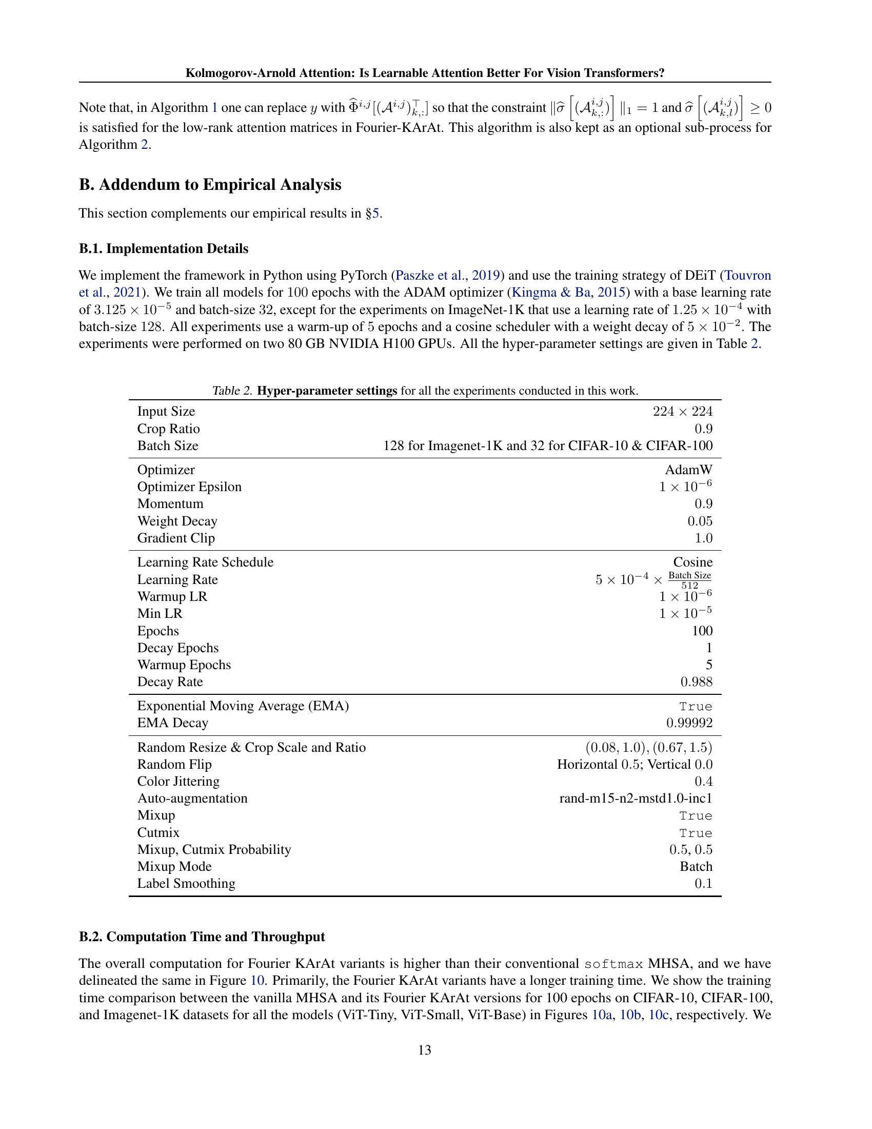
🔼 This table details the settings of all hyperparameters used in the experiments presented in the paper. It covers aspects like input image size, cropping ratio, batch size, the optimizer used (AdamW), optimizer settings (epsilon, momentum, weight decay, gradient clipping), learning rate scheduling, learning rate values (base, warmup, minimum), number of epochs, decay epochs, warmup epochs, decay rate, exponential moving average (EMA) parameters, random resize and crop specifications, random flipping probabilities, color jittering strength, auto-augmentation parameters, mixup and cutmix settings, label smoothing, and mixup mode. This comprehensive list allows for reproducibility of the experimental results.
read the caption
Table 2: Hyper-parameter settings for all the experiments conducted in this work.
| Model | Acc.@1 | |
|---|---|---|
| CIFAR-10 | CIFAR-100 | |
| ViT-Base | 83.45 | 58.07 |
| + | 81.81 | 55.92 |
| + | 80.75 | 57.36 |
| + | 80.09 | 56.01 |
| + | 81.00 | 57.15 |
| + | 79.80 | 54.83 |
| + | 81.17 | 56.38 |
| + | 50.47 | 42.02 |
| + | 40.74 | 39.85 |
| ViT-Small | 81.08 | 53.47 |
| + | 79.00 | 53.07 |
| + | 66.18 | 53.86 |
| + | 79.78 | 54.11 |
| + | 79.52 | 53.86 |
| + | 78.64 | 53.42 |
| + | 78.75 | 54.21 |
| + | 77.39 | 52.62 |
| + | 78.57 | 53.35 |
| ViT-Tiny | 72.76 | 43.53 |
| + | 75.75 | 45.77 |
| + | 74.94 | 46.00 |
| + | 76.69 | 46.29 |
| + | 75.56 | 46.75 |
| + | 75.85 | – |
| + | 74.71 | – |
| + | 75.11 | – |
| + | 74.45 | – |
| + | 74.85 | – |
| + | 73.97 | – |
| + | 74.52 | – |
| + | 73.58 | – |
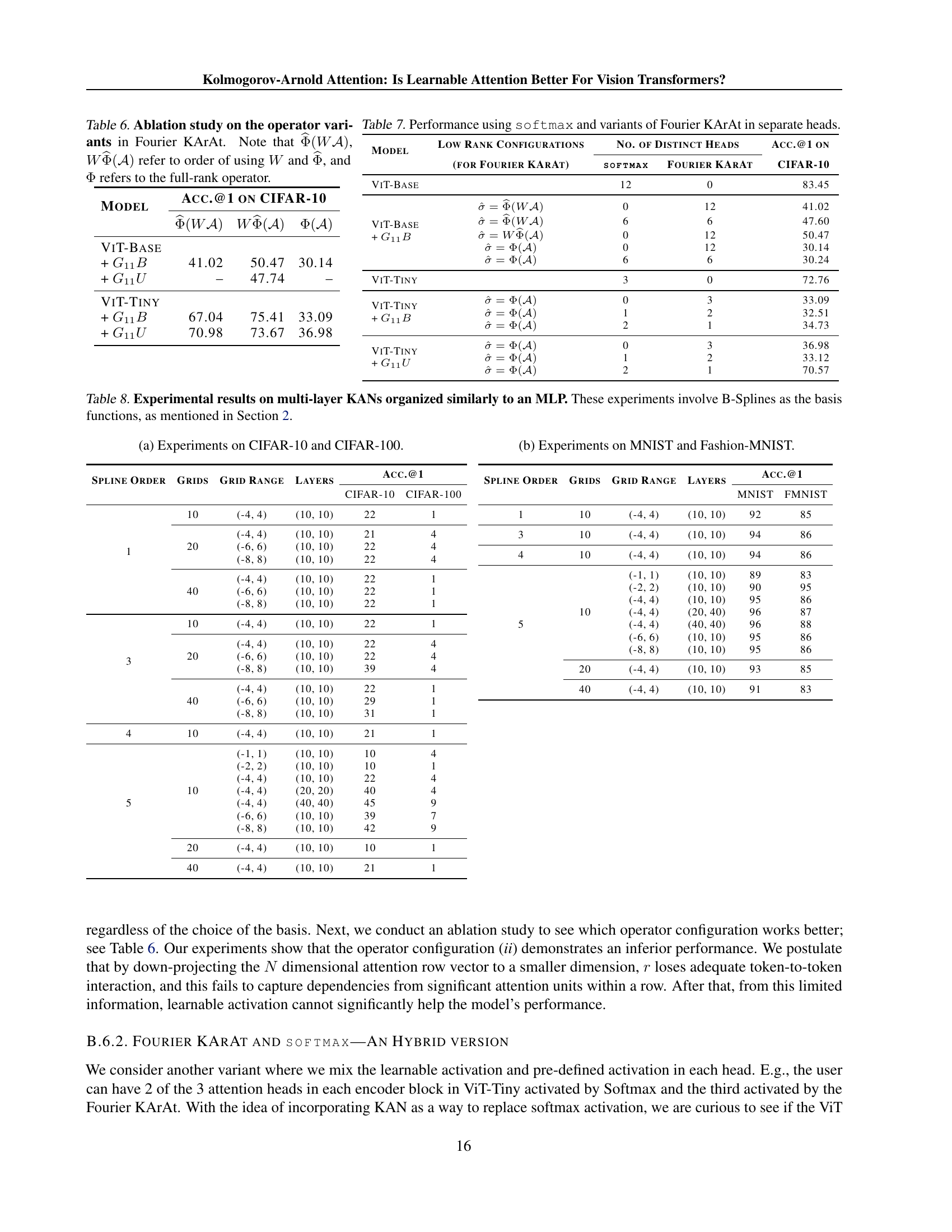
🔼 This table presents the performance of multi-layer Kolmogorov-Arnold Networks (KANs) structured like Multi-Layer Perceptrons (MLPs), using B-Spline basis functions. The results are organized to show how accuracy varies with different hyperparameters such as spline order, number of grids, grid range, and number of layers. The experiments were conducted on the CIFAR-10, CIFAR-100, MNIST, and Fashion-MNIST datasets. This allows for an analysis of how well the KAN architecture, typically used in simpler settings, generalizes to more complex image classification problems.
read the caption
Table 8: Experimental results on multi-layer KANs organized similarly to an MLP. These experiments involve B-Splines as the basis functions, as mentioned in Section 2.
Full paper#