TL;DR#
Auto-Regressive Video Diffusion Models (ARVDM) have shown promise in generating realistic videos, yet lack theoretical analysis. This work introduces Meta-ARVDM, a framework for analyzing ARVDMs. It uncovers two key issues: error accumulation (errors increase over time) and a memory bottleneck (models struggle to retain past information). Error accumulation refers to the fact that the later generated frames usually have poorer equality than the previous. By deriving an information-theoretic impossibility result, it shows that the memory bottleneck phenomenon cannot be avoided.
To address the memory bottleneck, the paper designs network structures to explicitly utilize more past frames, improving the performance. These structures leverage prepending and channel concatenation. The trade-off between mitigating the bottleneck and inference efficiency is improved by compressing frames. Experiments validate these methods and demonstrate a Pareto-frontier between error accumulation and the memory bottleneck across different methods. A project webpage is provided with supplementary material.
Key Takeaways#
Why does it matter?#
This paper provides a theoretical foundation and error analysis for ARVDMs, offering insights into memory bottlenecks and error accumulation that will help the community develop more efficient and effective models for long-form video generation. Also, the proposed Meta-ARVDM framework will help researchers analyze other ARVDMs. By addressing the limitations of existing models, this work paves the way for generating high-quality, coherent videos with reduced computational cost and improved temporal consistency, advancing the state-of-the-art in video synthesis.
Visual Insights#

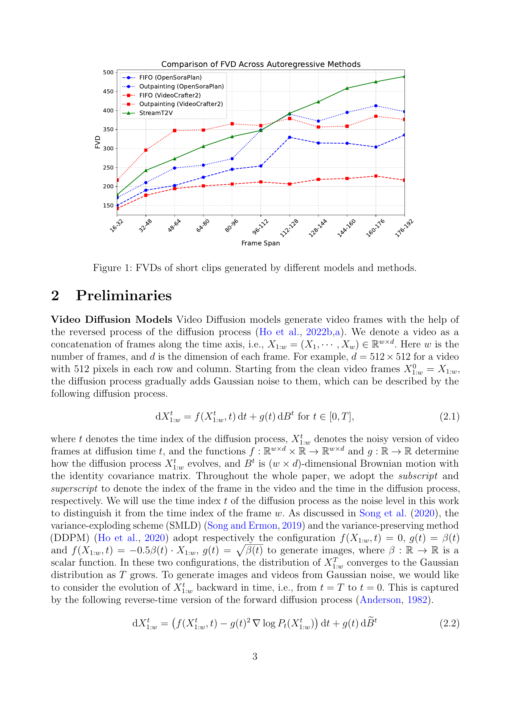
🔼 This figure compares the Frechet Video Distance (FVD) scores of short video clips (16 frames) generated by various autoregressive video diffusion models. The FVD measures the dissimilarity between the generated videos and real videos. Lower FVD indicates better generation quality. The x-axis represents the time span of frames (from start to end of the clip) and the y-axis shows the FVD scores. By analyzing the trends of FVD across different time spans, we can understand how different models handle the accumulation of errors during autoregressive generation. The graph shows that FVD generally increases over time, indicating that error accumulation is an inherent challenge in autoregressive video generation.
read the caption
Figure 1: FVDs of short clips generated by different models and methods.
| Memory Length | Compression | Network Memory Budget | 0-16 | 16-48 | 48-112 |
| Prepend | |||||
| 16 | N/A | N/A | 0.52 | 0.03 | 0.00 |
| 48 | N/A | N/A | 0.44 | 0.32 | 0.00 |
| 112 | N/A | N/A | 0.48 | 0.28 | 0.23 |
| 48 | joint | 8 | 0.28 | 0.22 | 0.00 |
| 48 | joint | 16 | 0.36 | 0.25 | 0.00 |
| 48 | joint | 32 | 0.44 | 0.28 | 0.00 |
| 48 | joint | 48 | 0.40 | 0.34 | 0.00 |
| Channel Concat | |||||
| 16 | N/A | N/A | 0.24 | 0.03 | 0.00 |
| 48 | N/A | N/A | 0.16 | 0.19 | 0.00 |
| 112 | N/A | N/A | 0.12 | 0.13 | 0.08 |
| 48 | modulated | 8 | 0.16 | 0.16 | 0.00 |
| 48 | modulated | 16 | 0.20 | 0.19 | 0.00 |
| 48 | modulated | 32 | 0.24 | 0.22 | 0.00 |
| 48 | modulated | 48 | 0.28 | 0.22 | 0.00 |
| Cross Attention | |||||
| 112 | N/A | N/A | 0.00 | 0.00 | 0.00 |
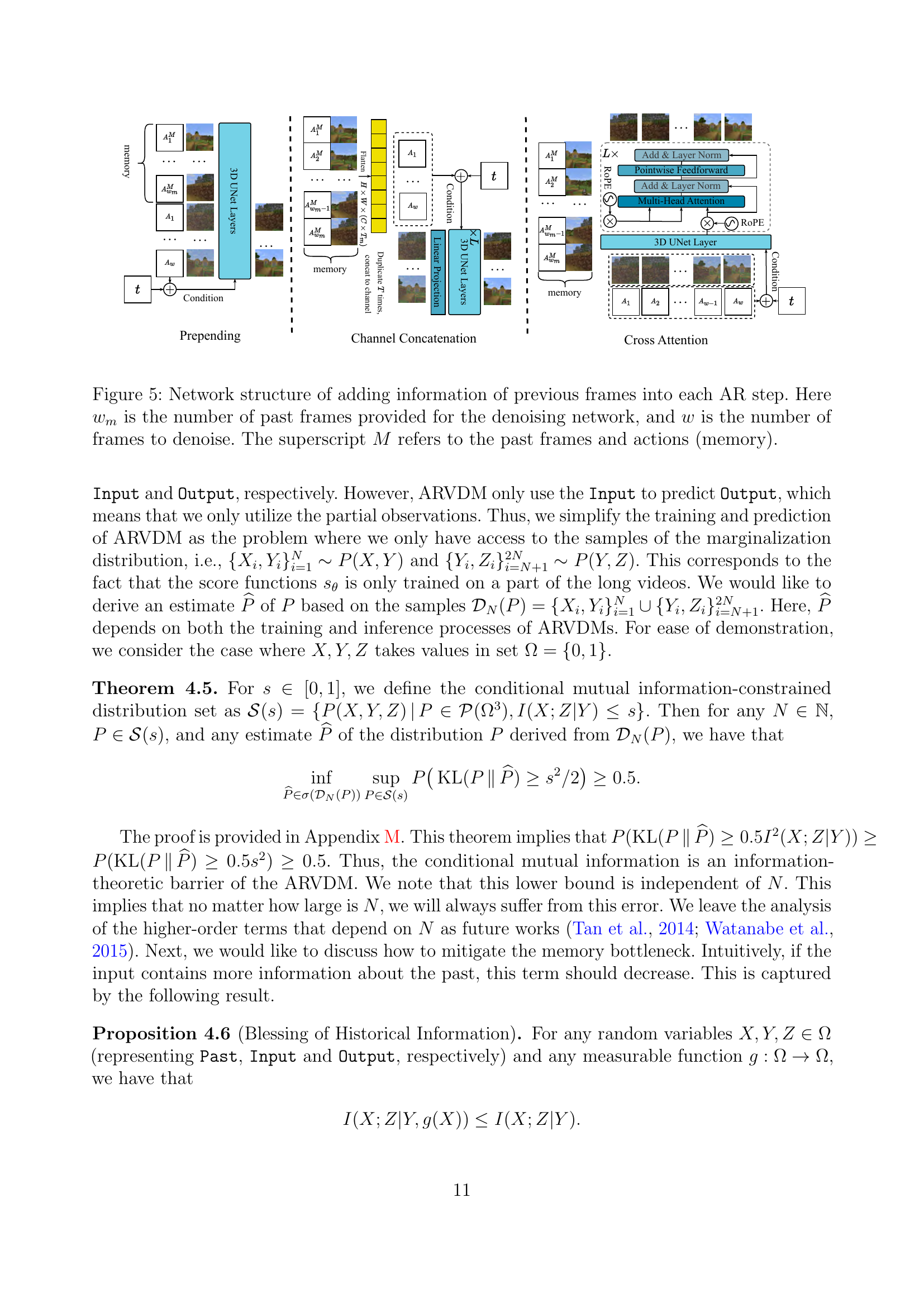
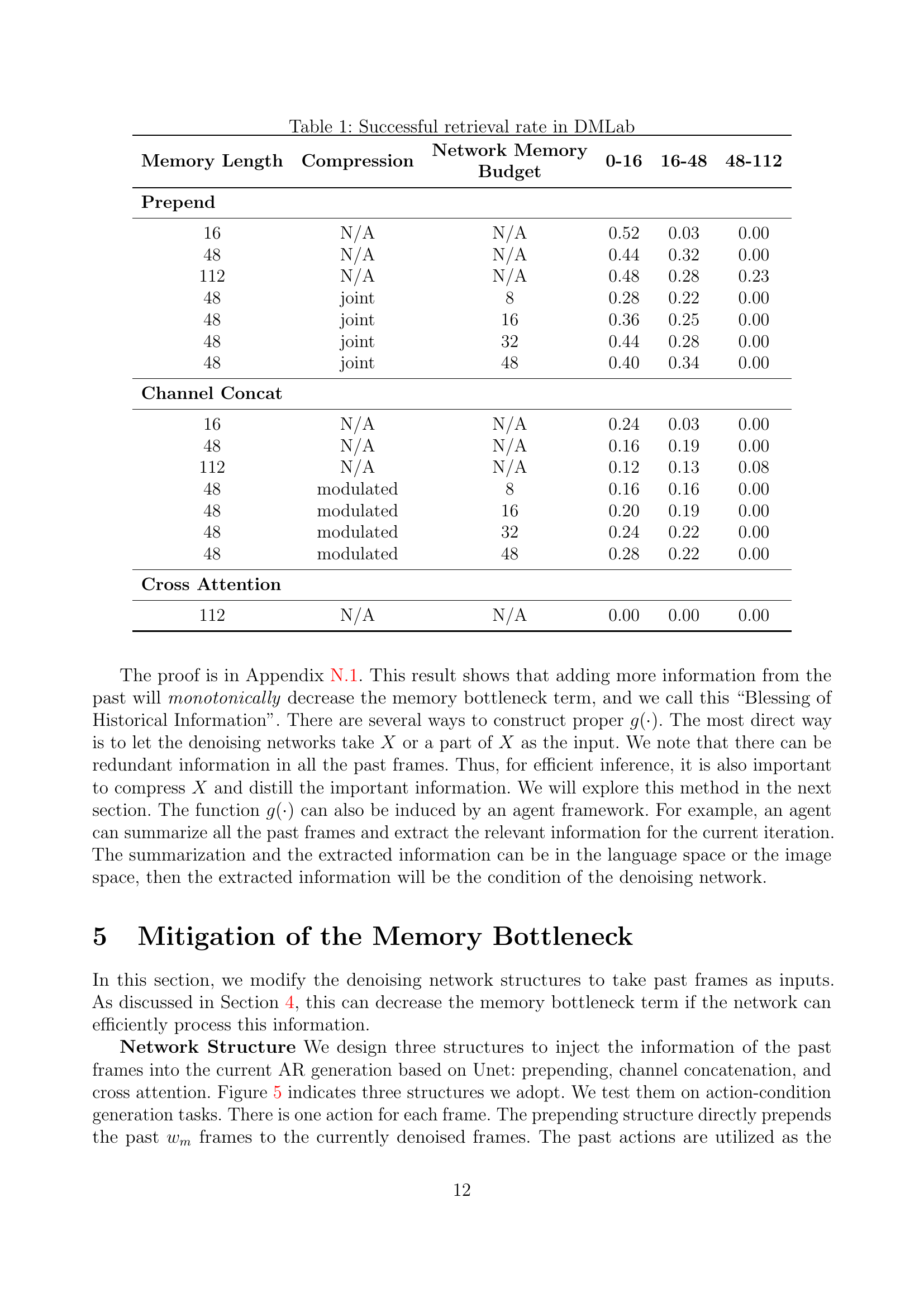
🔼 This table presents the success rates of retrieving past frames in the DMLab environment using different network architectures and memory sizes. The experiment tests the ability of the models to recall previously seen scenes. The table shows the results for three different memory lengths (16, 48, and 112 frames), with and without compression. Three different network structures are evaluated: prepending, channel concatenation, and cross-attention. The results are broken down into three time intervals (0-16, 16-48, 48-112 frames) to analyze how effectively the models can recall information from the past. The ‘Network Memory Budget’ column indicates the number of parameters in the network.
read the caption
Table 1: Successful retrieval rate in DMLab
In-depth insights#
ARVDM:Meta-View#
While “ARVDM: Meta-View” isn’t explicitly present, we can discuss its potential meaning within the paper’s context. A meta-view of ARVDMs suggests a higher-level perspective that unifies different ARVDM architectures. It would involve identifying common underlying principles and abstracting away implementation details. This meta-view could offer a framework for understanding ARVDM behavior, analyzing their limitations (like error accumulation), and designing improvements. It would focus on the core auto-regressive process, the diffusion model components, and how they interact. This framework also makes explicit assumptions to make AR generation plausible. A Meta-View serves as firm basis for common shared characteristics across most ARVDMs. By analyzing the core learning algorithm we can discover types of errors across the long video generation process.
Error Breakdown#
Analyzing the ‘Error Breakdown’ in autoregressive video diffusion models (ARVDMs) reveals a complex interplay of factors degrading video quality. Error sources such as noise initialization, score estimation inaccuracies, and discretization during the diffusion process compound over time, a phenomenon known as error accumulation. Uniquely, ARVDMs face a memory bottleneck, limiting their ability to maintain long-term coherence and consistency. This arises from the model’s imperfect retention of past frames, leading to inconsistencies. Overcoming this bottleneck necessitates architectural modifications to incorporate past frames more effectively. The research also derives an information-theoretic lower bound. It shows that the memory bottleneck is inevitable, highlighting a fundamental constraint in ARVDMs, and proposes various methods to mitigate this memory bottleneck. These methods involve different network structures to use more past frames and compressing frames to improve inference efficiency.The trade-off between mitigation of the memory bottleneck and the inference efficiency is significantly improved.
Mem. Bottleneck#
The memory bottleneck in ARVDMs is a critical issue, causing inconsistency across AR steps. It arises because the model struggles to retain information from past frames, hindering its ability to generate coherent videos. This limitation stems from the score function’s inability to fully incorporate historical data during denoising, leading to a reliance on immediate inputs. This bottleneck is theoretically unavoidable, as shown through information-theoretic bounds. To mitigate this, the researchers propose network structures that explicitly incorporate more past frames as input, such as prepending, channel concatenation, and cross-attention mechanisms. Furthermore, they explore compression techniques to balance the incorporation of historical information with inference efficiency. The goal is to enhance the model’s memory capacity, thus facilitating better context retention and improved long-term video coherence.
Past Frame Boost#
Leveraging past frames seems crucial for enhancing video generation quality, especially in autoregressive models. The key idea is injecting temporal consistency by utilizing information from previous frames. This can be achieved by either directly incorporating the raw pixels or features extracted from them into the current frame’s generation process. The effectiveness hinges on efficient information compression and integration. Network architectures should be able to selectively attend to and combine relevant details from past frames. A careful balance needs to be struck between increased computational cost and improved generation quality when incorporating past frames.
Future Work#
Future work could explore several avenues to enhance ARVDMs. Lower bounds for error accumulation need investigation for tighter performance guarantees. The memory bottleneck’s lower bound could be refined for better theoretical understanding, the compression module could explore state-space models like Mamba beyond transformers for improved efficiency. Further research could focus on more sophisticated summarization techniques using agent frameworks to extract relevant information from past frames. Addressing the challenges of long-range dependencies and high computational costs associated with these models is crucial. Moreover, exploring the use of alternative architectures and loss functions could lead to more efficient and robust ARVDMs.
More visual insights#
More on figures

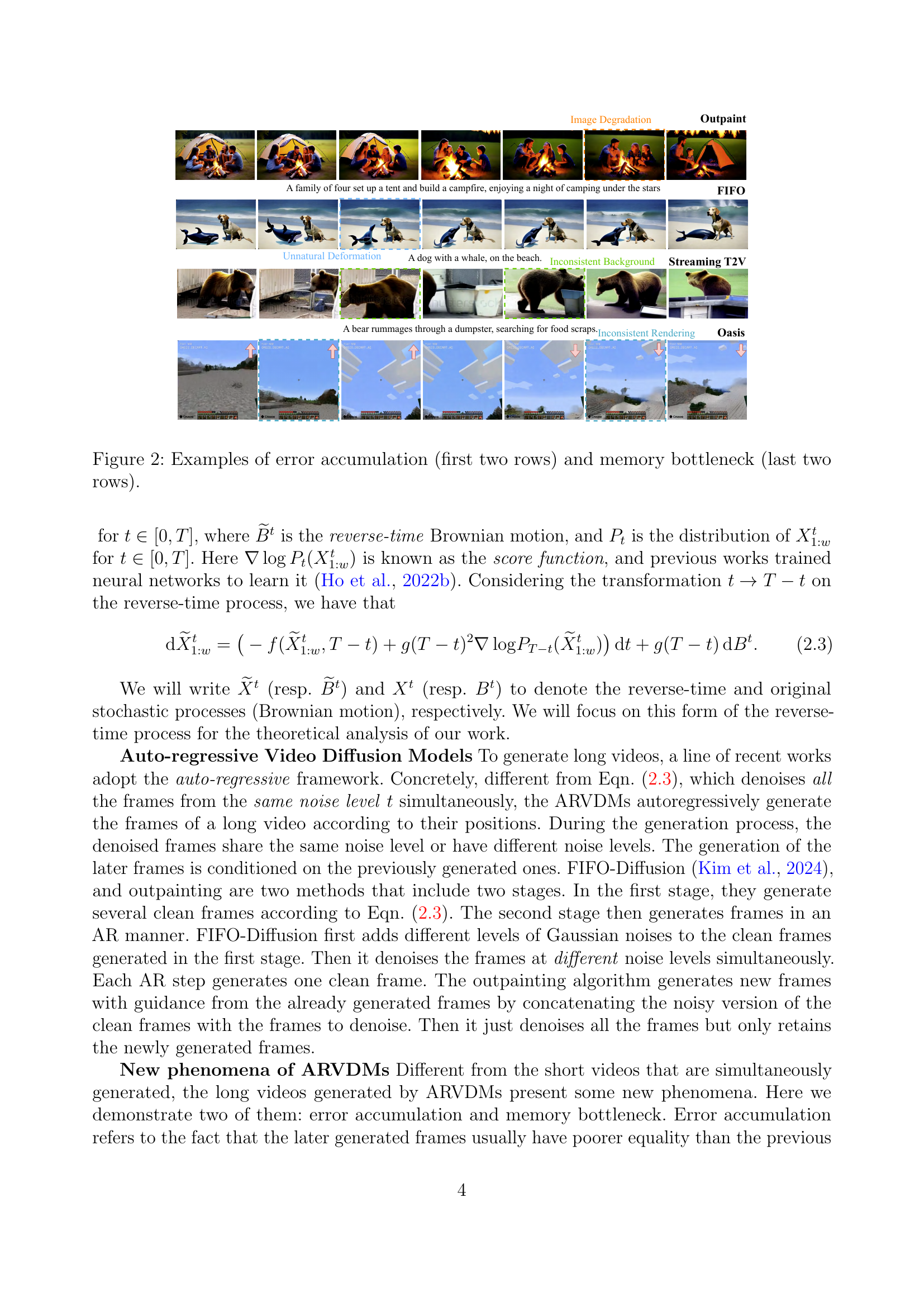
🔼 This figure provides visual examples of two main error types affecting Auto-Regressive Video Diffusion Models (ARVDMs). The top two rows showcase error accumulation, where errors compound over time as the model generates subsequent frames of a video. The generated frames become increasingly inconsistent or distorted. The bottom two rows illustrate the memory bottleneck phenomenon, where the model fails to retain and utilize information from earlier frames in the sequence, leading to inconsistencies between frames. The memory bottleneck is specific to ARVDMs that generate long videos, and these errors are not present in video models that process all frames simultaneously.
read the caption
Figure 2: Examples of error accumulation (first two rows) and memory bottleneck (last two rows).
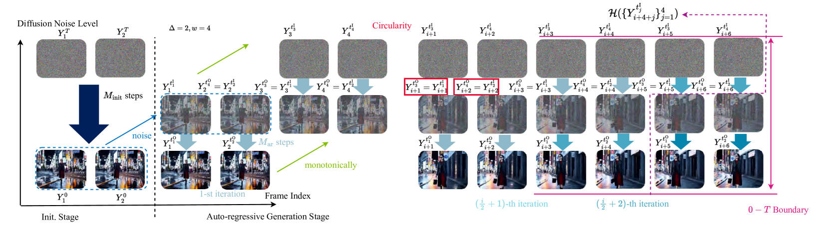
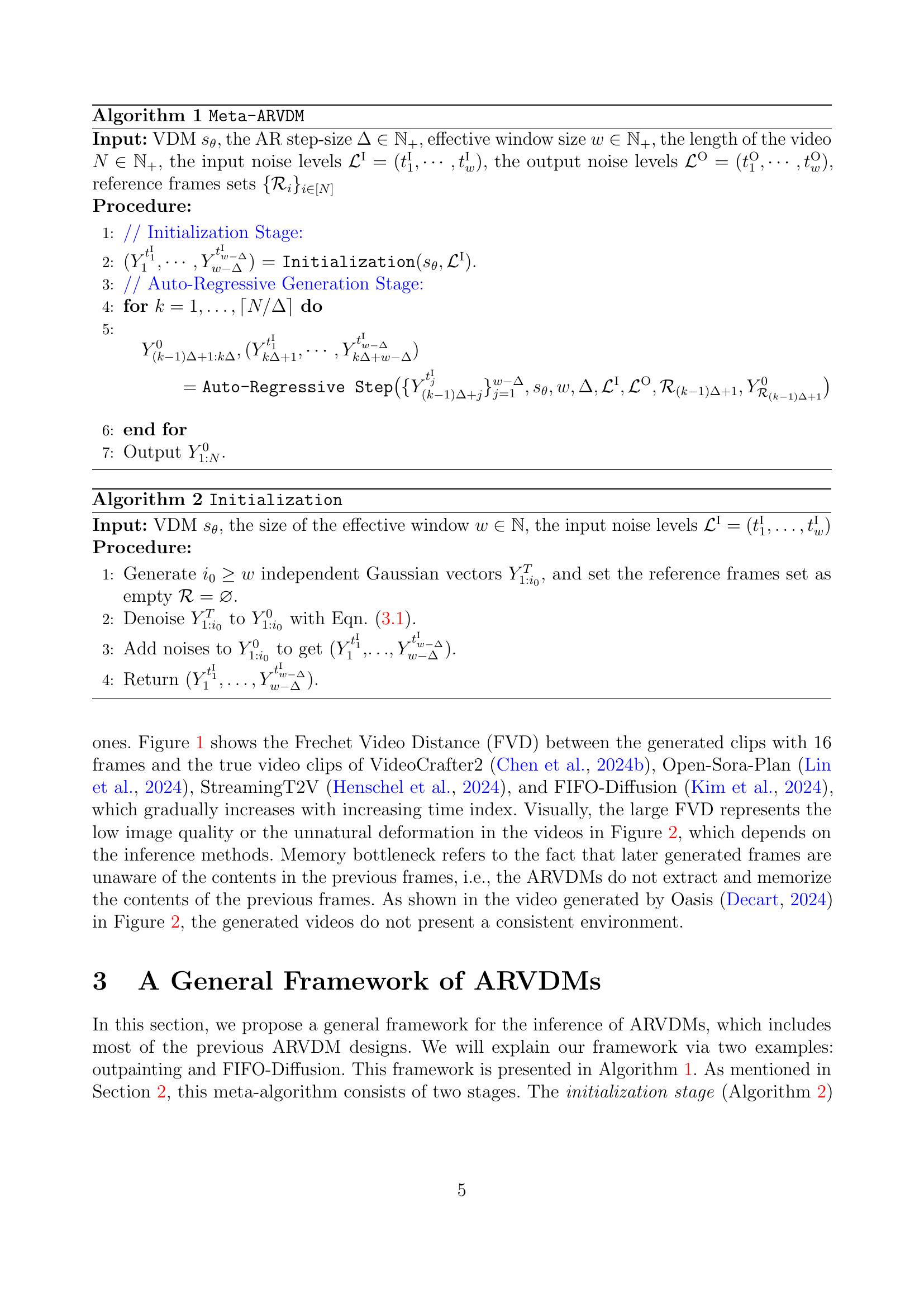
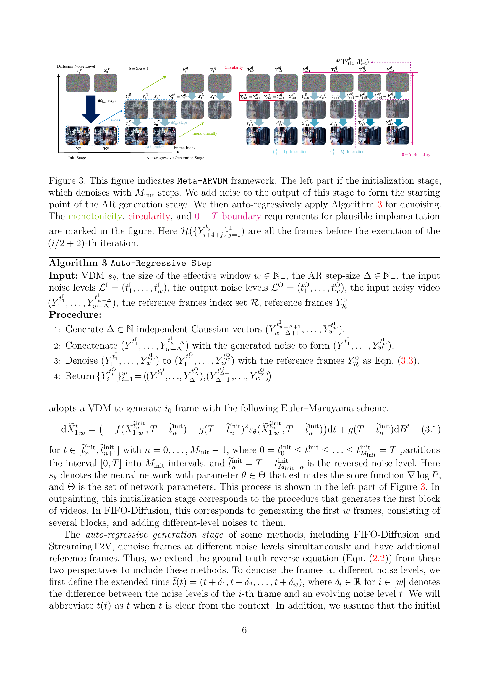
🔼 Figure 3 illustrates the Meta-ARVDM framework, a unified framework encompassing most existing autoregressive video diffusion models (ARVDMs). The figure is divided into two main stages: initialization and autoregressive generation. The initialization stage begins with denoising using a certain number of steps (Minit). The output is then noised to form the starting point for the autoregressive generation stage. This stage iteratively applies Algorithm 3 to further denoise, generating subsequent frames. Key properties of the ARVDM generation process—monotonicity, circularity, and 0-T boundary conditions—are visually represented and highlighted in the figure. The notation ℋ({Yi+4+jtjI}j=14) represents all frames preceding the (i/2+2)-th iteration step, which is crucial for understanding the autoregressive process.
read the caption
Figure 3: This figure indicates Meta-ARVDM framework. The left part if the initialization stage, which denoises with Minitsubscript𝑀initM_{{\text{init}}}italic_M start_POSTSUBSCRIPT init end_POSTSUBSCRIPT steps. We add noise to the output of this stage to form the starting point of the AR generation stage. We then auto-regressively apply Algorithm 3 for denoising. The monotonicity, circularity, and 0−T0𝑇0-T0 - italic_T boundary requirements for plausible implementation are marked in the figure. Here ℋ({Yi+4+jtjI}j=14)ℋsuperscriptsubscriptsuperscriptsubscript𝑌𝑖4𝑗superscriptsubscript𝑡𝑗I𝑗14\mathcal{H}(\{Y_{i+4+j}^{t_{j}^{\mathrm{I}}}\}_{j=1}^{4})caligraphic_H ( { italic_Y start_POSTSUBSCRIPT italic_i + 4 + italic_j end_POSTSUBSCRIPT start_POSTSUPERSCRIPT italic_t start_POSTSUBSCRIPT italic_j end_POSTSUBSCRIPT start_POSTSUPERSCRIPT roman_I end_POSTSUPERSCRIPT end_POSTSUPERSCRIPT } start_POSTSUBSCRIPT italic_j = 1 end_POSTSUBSCRIPT start_POSTSUPERSCRIPT 4 end_POSTSUPERSCRIPT ) are all the frames before the execution of the (i/2+2)𝑖22(i/2+2)( italic_i / 2 + 2 )-th iteration.

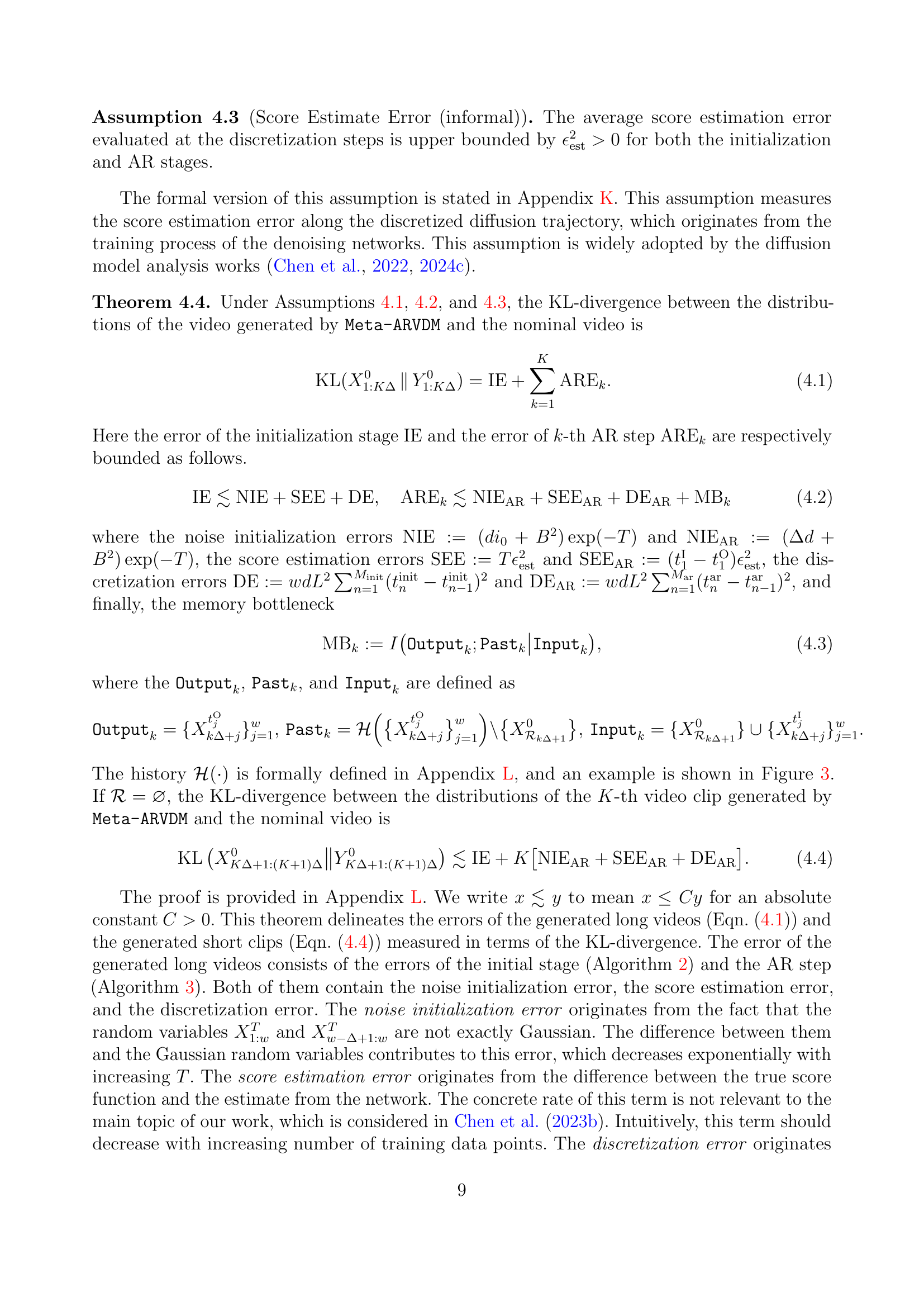
🔼 This figure simplifies the scenario for proving the lower bound of the error in autoregressive video diffusion models. It illustrates a Markov chain representing the relationship between the past frames (X), the input frames (Y), and the output frames (Z). This simplification is used to demonstrate that the memory bottleneck inherent in autoregressive models is unavoidable due to information loss.
read the caption
Figure 4: The simplified setting for the proof of lower bounds.

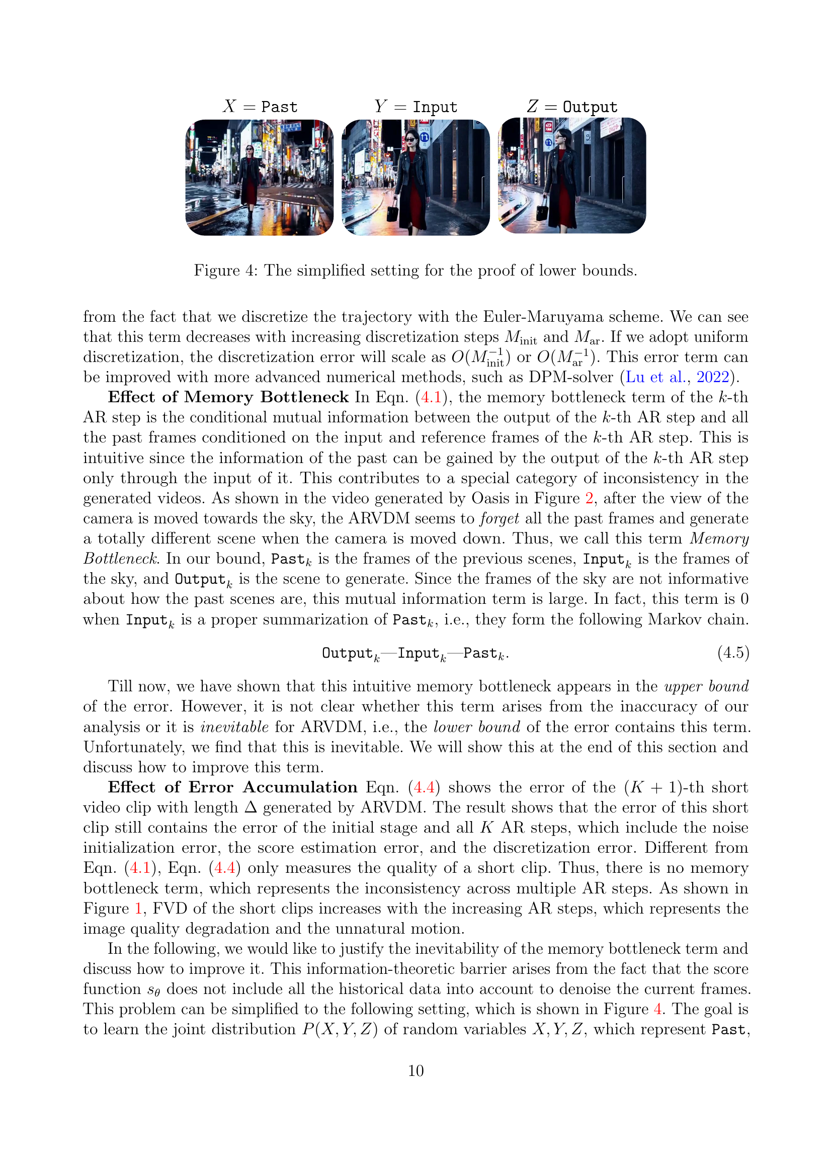
🔼 Figure 5 illustrates the architecture of the network designed to incorporate information from previous frames into each autoregressive (AR) step during video generation. The core concept is to leverage the temporal context of the video, avoiding the limitations of only considering the current frame. The network takes two key inputs: the frames currently being processed (‘w’ frames) and the preceding frames from the video’s history (‘wm’ frames), along with their corresponding actions. The superscript ‘M’ indicates the incorporation of both past frames and actions into the model’s memory. This enriched context allows the model to better predict the next frames in the sequence, improving temporal consistency and mitigating the ‘memory bottleneck’ problem associated with autoregressive models that process videos frame-by-frame.
read the caption
Figure 5: Network structure of adding information of previous frames into each AR step. Here wmsubscript𝑤𝑚w_{m}italic_w start_POSTSUBSCRIPT italic_m end_POSTSUBSCRIPT is the number of past frames provided for the denoising network, and w𝑤witalic_w is the number of frames to denoise. The superscript M𝑀Mitalic_M refers to the past frames and actions (memory).

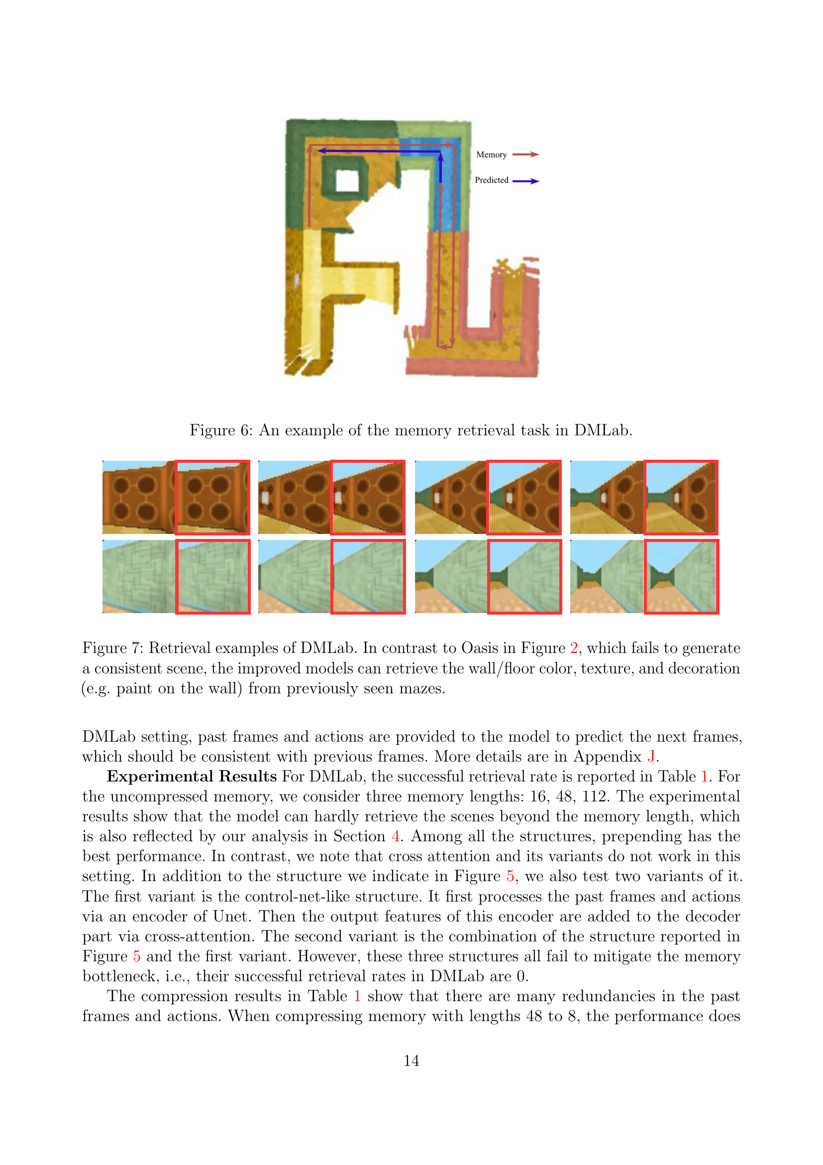
🔼 This figure illustrates a memory retrieval task within the DMLab environment. The objective is to assess the model’s ability to recall and utilize information from previous frames to accurately generate subsequent frames. The left side displays the ground truth sequence of frames, while the right side shows the model’s generated frames based on the provided context. This test evaluates the model’s capacity for long-term memory and consistency in generating temporally coherent video.
read the caption
Figure 6: An example of the memory retrieval task in DMLab.

🔼 Figure 7 showcases retrieval examples from the DMLab environment. The improved models, unlike the Oasis model in Figure 2, successfully generate consistent scenes. This consistency demonstrates the models’ ability to recall and accurately reproduce specific visual details from previously encountered maze environments. These details include the colors of walls and floors, the textures of surfaces, and decorative elements such as paint on walls. The successful reproduction highlights the models’ improved memory and ability to maintain coherence across generated video frames, which is a significant step towards improved video generation capabilities.
read the caption
Figure 7: Retrieval examples of DMLab. In contrast to Oasis in Figure 2, which fails to generate a consistent scene, the improved models can retrieve the wall/floor color, texture, and decoration (e.g. paint on the wall) from previously seen mazes.

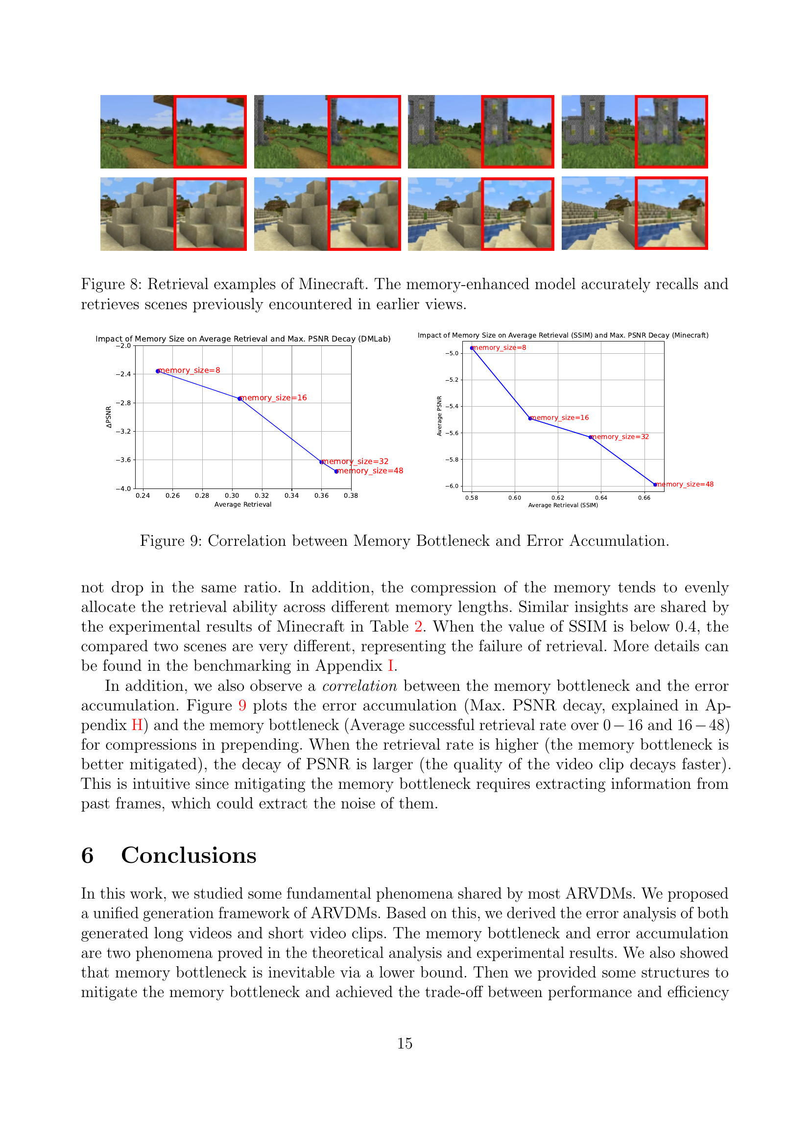
🔼 This figure showcases retrieval examples from the Minecraft environment, demonstrating the capability of a memory-enhanced model. The images depict various scenes from the game. The model, having been trained with enhanced memory capabilities, accurately recalls and retrieves scenes encountered earlier, highlighting its improved ability to maintain context and consistency over longer sequences of video generation.
read the caption
Figure 8: Retrieval examples of Minecraft. The memory-enhanced model accurately recalls and retrieves scenes previously encountered in earlier views.

🔼 This figure visualizes the relationship between memory bottleneck and error accumulation in autoregressive video diffusion models. The x-axis represents the average retrieval rate (a metric indicating the model’s ability to recall past information), and the y-axis represents the maximum PSNR decay (a measure of the increase in error over time). The plot shows that when the memory bottleneck is effectively mitigated (higher average retrieval rate), the error accumulation is greater (larger PSNR decay). This indicates a trade-off between these two aspects of model performance. Different memory sizes (8, 16, 32, and 48) are compared separately for both DMLab and Minecraft datasets.
read the caption
Figure 9: Correlation between Memory Bottleneck and Error Accumulation.

🔼 This figure showcases the model’s performance on the DMLab environment. Each pair of images shows the expected ground truth (left) alongside the model’s generated output (right, outlined in red). The goal is to assess the model’s ability to accurately recall and reconstruct visual scenes from memory. The figure helps to visually demonstrate the effectiveness (or lack thereof) of the model in maintaining visual consistency across time steps. The red box highlights differences between the model’s output and the ground truth, allowing for quick visual comparison and evaluation.
read the caption
Figure 10: Recall demonstrations on DMLab. The left frames represent the expected ground truth, while the right frames, outlined with a red square, are generated by the model.

🔼 This figure showcases the model’s ability to generate video frames in Minecraft, given a sequence of initial frames as context. The left column displays the ground truth frames (what the model ideally should produce), while the right column shows the frames generated by the model. The red boxes highlight the frames generated by the model, which are being evaluated for accuracy against the ground truth. The first four frames in each row (without red boxes) serve as the input context for the model; they are not generated by the model but are provided as a starting point. This visual comparison demonstrates the model’s capacity to maintain temporal coherence and generate realistic frames but also reveals instances where it falls short.
read the caption
Figure 11: Recall demonstrations on Minecraft. The left frames represent the expected ground truth, while the right frames, outlined with a red square, are generated by the model. The first 4 frames without red squares are provided context.

🔼 This figure illustrates two distinct network architectures designed for compressing past frames and actions within a video generation model. The left panel showcases the ‘joint’ method, where past frames and actions are concatenated and processed together through feedforward, spatial, and temporal attention modules. The right panel depicts the ‘modulated’ method. Here, actions modulate the frames before processing through similar modules. Both methods employ compression by retaining only the final, compressed representations of frames and actions, improving efficiency. These compressed representations are then integrated into subsequent video generation steps.
read the caption
Figure 12: The network structure adopted to compress the past frames and actions.

🔼 This figure visualizes pairs of frames from Minecraft video trajectories, categorized by their Structural Similarity Index (SSIM) scores. The SSIM score quantifies the visual similarity between two images; higher scores indicate greater similarity. The figure showcases examples across different SSIM ranges: low (SSIM < 0.4), medium (0.4 ≤ SSIM < 0.7), high (0.7 ≤ SSIM < 0.9), and near-identical (SSIM ≥ 0.9). Each range illustrates the visual differences (or lack thereof) between the frame pairs, demonstrating how SSIM captures various levels of visual similarity, from nearly indistinguishable to quite different scenes.
read the caption
Figure 13: Minecraft Example Pairs from Minecraft Across Varying SSIM Score Ranges

🔼 This figure illustrates the sets 𝒢(⋅) and ℋ(⋅) used in the proof of Theorem 4.4, which analyzes the KL-divergence between the generated and true videos. Specifically, it shows how these sets capture the evolution of noise levels and the denoising process during autoregressive video generation. The figure uses the examples of Δ=2 and ω=4 to illustrate how the sets are built from the noisy video frames, the reference frames, and the results of applying autoregressive steps. It visualizes the sets of generated random vectors, both inputs and outputs, which are progressively concatenated across iterations of the autoregressive step. The diagrams visually explain the mathematical notations representing these sets.
read the caption
Figure 14: The examples of 𝒢(⋅)𝒢⋅\mathcal{G}(\cdot)caligraphic_G ( ⋅ ) and ℋ(⋅)ℋ⋅\mathcal{H}(\cdot)caligraphic_H ( ⋅ ).
More on tables
| Context Length | Compression | Network Memory Budget | 0-16 | 16-48 | 48-112 |
| Prepend | |||||
| 16 | N/A | N/A | 0.75 | 0.39 | 0.37 |
| 48 | N/A | N/A | 0.74 | 0.62 | 0.35 |
| 112 | N/A | N/A | 0.72 | 0.60 | 0.55 |
| 48 | joint | 8 | 0.63 | 0.53 | 0.38 |
| 48 | joint | 16 | 0.67 | 0.55 | 0.37 |
| 48 | joint | 32 | 0.70 | 0.57 | 0.38 |
| 48 | joint | 48 | 0.72 | 0.61 | 0.35 |
| Channel Concat | |||||
| 16 | N/A | N/A | 0.61 | 0.38 | 0.38 |
| 48 | N/A | N/A | 0.58 | 0.57 | 0.37 |
| 112 | N/A | N/A | 0.59 | 0.56 | 0.51 |
| 48 | modulated | 8 | 0.54 | 0.53 | 0.36 |
| 48 | modulated | 16 | 0.56 | 0.54 | 0.35 |
| 48 | modulated | 32 | 0.57 | 0.56 | 0.36 |
| 48 | modulated | 48 | 0.57 | 0.57 | 0.37 |
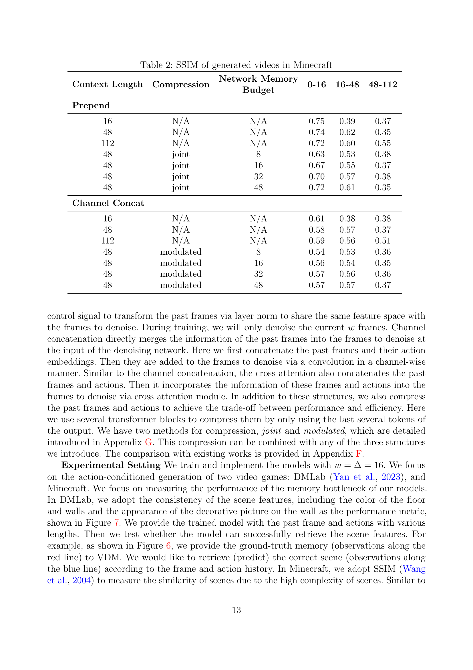
🔼 This table presents the Structural Similarity Index (SSIM) scores for videos generated using different models and parameters in the Minecraft environment. SSIM is a metric used to measure the perceptual similarity between two images or videos. The table shows SSIM values broken down by context length (number of preceding frames considered), compression technique (whether compression of past frames was applied and how), network memory budget, and three time intervals (0-16, 16-48, 48-112 frames). This allows for analysis of how different approaches affect the quality of generated videos in Minecraft. Lower SSIM scores indicate lower perceived quality.
read the caption
Table 2: SSIM of generated videos in Minecraft
| Network Memory Budget | 0–16 | 16–32 | 32–48 | 48–64 |
| 8 | 10.24 | 9.47 | 8.83 | 7.88 |
| 16 | 10.14 | 8.81 | 8.24 | 7.39 |
| 32 | 10.46 | 8.19 | 7.82 | 6.83 |
| 48 | 10.52 | 8.00 | 7.58 | 6.76 |
🔼 This table presents the results of an error accumulation analysis performed on the DMLab dataset. The analysis focuses on the Peak Signal-to-Noise Ratio (PSNR) metric, measuring the difference in image quality between generated video clips and ground truth videos. It shows how error accumulates over time (frames). Different network memory budgets (8, 16, 32, and 48) are compared, and PSNR is calculated for four frame intervals (0-16, 16-32, 32-48, and 48-64) to assess the degradation of video quality as more frames are generated.
read the caption
Table 3: Error Accumulation on DMLab (PSNR)
| Network Memory Budget | 0–16 | 16–32 | 32–48 | 48–64 |
| 8 | 15.25 | 13.43 | 11.39 | 10.29 |
| 16 | 15.47 | 12.92 | 11.10 | 9.98 |
| 32 | 15.36 | 12.64 | 11.01 | 9.73 |
| 48 | 15.46 | 12.31 | 10.57 | 9.47 |
🔼 This table presents the Peak Signal-to-Noise Ratio (PSNR) values, showcasing error accumulation in video generation across different memory budget settings within the Minecraft environment. The PSNR values are calculated for four time intervals (0-16, 16-32, 32-48, and 48-64 frames) of generated video sequences. Each row represents a different memory budget setting (8, 16, 32, and 48), illustrating the change in PSNR over time. A decreasing trend in PSNR over these time intervals suggests that the error accumulates as the model generates longer video sequences. The magnitude of the decrease indicates the severity of error accumulation. Comparing the PSNR values across the memory budget rows allows an assessment of how the memory budget affects error accumulation during video generation.
read the caption
Table 4: Error Accumulation on Minecraft (PSNR)
Full paper#