TL;DR#
Earth observation (EO) foundation models have great potential, but current models have limitations such as fixed spectral sensors, focus on Earth’s surface, and neglecting metadata. This paper takes a step towards next-generation EO foundation models. To address this, the authors created Copernicus-Pretrain, a massive dataset of 18.7M aligned images from Copernicus Sentinel missions covering Earth’s surface and atmosphere. The dataset enables comprehensive modeling of Earth system interactions.
Building on this dataset, the authors developed Copernicus-FM, a model that handles any spectral or non-spectral sensor via dynamic hypernetworks. The model architecture enhances flexibility by adapting to different data inputs and supports metadata integration. They also established Copernicus-Bench, a benchmark with 15 tasks for evaluating model performance across Sentinel missions. It facilitates the systematic assessment of foundation models across various practical applications, promoting a versatile approach to EO data processing.
Key Takeaways#
Why does it matter?#
This paper is important for researchers as it introduces a comprehensive framework for EO foundation models, addressing key limitations in sensor diversity, model flexibility, and evaluation breadth. It offers valuable resources for advancing research in EO, climate, and weather modeling, fostering interdisciplinary collaboration and innovation.
Visual Insights#

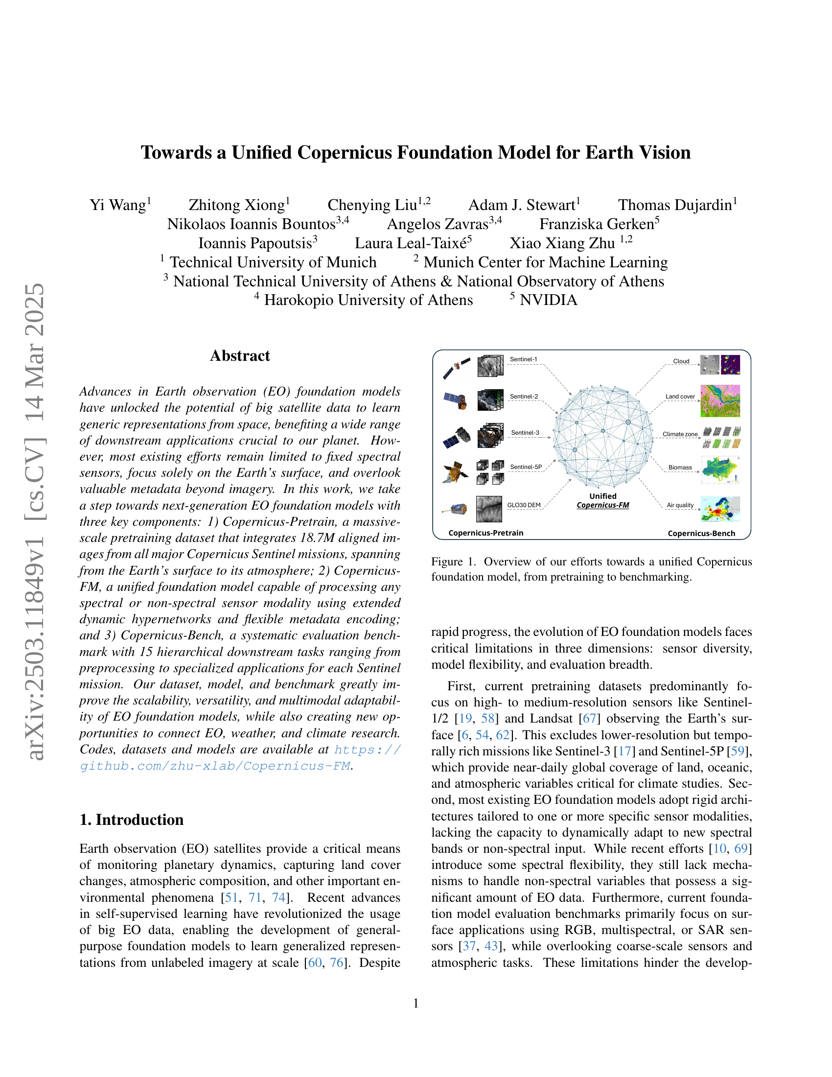
🔼 This figure illustrates the overall architecture of the proposed unified Copernicus foundation model for Earth vision. It starts with a massive pretraining dataset called Copernicus-Pretrain, which integrates data from various Copernicus Sentinel missions, encompassing the Earth’s surface and atmosphere. This data is used to train the Copernicus-FM foundation model, designed for processing diverse sensor modalities (spectral or non-spectral) using dynamic hypernetworks. Finally, this model is evaluated on a comprehensive benchmark, Copernicus-Bench, which includes various downstream tasks across multiple Sentinel missions.
read the caption
Figure 1: Overview of our efforts towards a unified Copernicus foundation model, from pretraining to benchmarking.
| Modality | GSD | Image size | # Grid cells | # Patches | # Timestamps | # Total images | |
|---|---|---|---|---|---|---|---|
| Sentinel-1 GRD | SAR | 10 m | 2642642 | 247,723 | 1,067,267 | 4 | 4,227,387 |
| Sentinel-2 TOA | MS | 10 m | 26426413 | 247,723 | 1,067,267 | 4 | 4,218,065 |
| Sentinel-3 OLCI | MS | 300 m | 969621 | 281,375 | 281,375 | 8 | 2,189,561 |
| Sentinel-5P CO | atmos. | 1 km | 2828 | 306,097 | 306,097 | 1–12 | 2,104,735 |
| Sentinel-5P NO2 | atmos. | 1 km | 2828 | 291,449 | 291,449 | 1–12 | 1,752,558 |
| Sentinel-5P SO2 | atmos. | 1 km | 2828 | 262,259 | 262,259 | 1–12 | 1,366,452 |
| Sentinel-5P O3 | atmos. | 1 km | 2828 | 306,218 | 306,218 | 1–12 | 2,556,631 |
| Copernicus DEM | elevation | 30 m | 960960 | 297,665 | 297,665 | 1 | 297,665 |
| Copernicus-Pretrain | 312,567 | 3,879,597 | 18,713,054 |
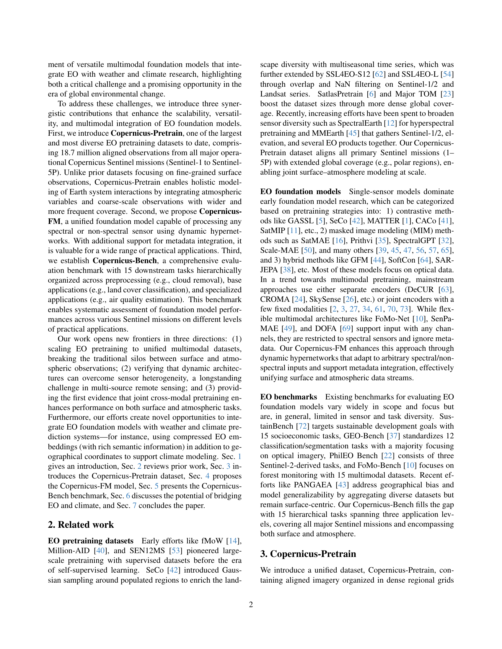
🔼 This table presents a statistical summary of the Copernicus-Pretrain dataset, a crucial component of the research. It details the number of grid cells, patches, and total images for each Sentinel mission included (Sentinel-1 GRD, Sentinel-2 TOA, Sentinel-3 OLCI, Sentinel-5P for various atmospheric variables (CO, NO2, SO2, O3), and Copernicus DEM). The table also specifies the ground sample distance (GSD) and image size for each sensor modality, providing a comprehensive overview of the dataset’s scale and diversity.
read the caption
Table 1: Copernicus-Pretrain dataset statistics.
In-depth insights#
EO Data Fusion#
EO data fusion is crucial for enhanced Earth observation insights. It involves integrating data from multiple sources to create a comprehensive view. Challenges include sensor heterogeneity and data alignment. Effective fusion improves accuracy and provides richer information, benefiting environmental monitoring and disaster response. Future advancements lie in multimodal foundation models and flexible architectures adapting to diverse data.
Copernicus-FM#
The Copernicus-FM section likely details the core architecture of the proposed foundation model. A key innovation probably lies in handling diverse sensor inputs (spectral/non-spectral) via dynamic hypernetworks, adapting to varying spatial resolutions. Metadata integration (geolocation, time) is a significant aspect, enhancing the model’s awareness. The pretraining objective combines masked image modeling (MIM) and continual distillation, improving representation quality and leveraging knowledge from models like DINOv2. The model seems designed for versatility across different Earth observation tasks and sensor types. Ablation studies likely validate the effectiveness of hypernetworks and metadata.
Dynamic HyperNets#
Dynamic Hypernetworks offer a promising avenue for creating flexible and adaptable models, especially in domains with diverse input modalities like Earth observation. The core idea is to use a hypernetwork to generate the weights of another network (the main network), allowing the model to dynamically adapt to different inputs. This is useful for EO tasks, where data can come from various sensors (optical, SAR, etc.) with differing spectral bands and resolutions. By conditioning the hypernetwork on the sensor characteristics, the main network can process diverse data types. Hypernetworks can also integrate metadata, such as geolocation and time, by encoding this information and using it to influence the weight generation process. This enables the model to be aware of the context of the input data, leading to improved performance. The challenge lies in designing efficient hypernetworks that can generate high-quality weights without adding excessive computational overhead.
Climate Bridging#
Climate bridging in Earth observation (EO) foundation models represents a paradigm shift, moving beyond isolated environmental analysis towards integrated Earth system understanding. By fusing EO data with weather and climate models, these models can leverage the wealth of satellite imagery and derived products to enhance climate prediction and monitoring. The potential lies in creating semantically rich geographical representations via EO-encoded grid embeddings, directly aligning with climate parameters from reanalysis datasets like ERA5. This integration not only refines climate models by incorporating visual context and detailed surface information but also opens avenues for improved medium-range weather forecasting by enriching static and dynamic climate variables with EO-derived insights. This cross-disciplinary approach offers a holistic view of planetary dynamics, crucial for addressing global environmental changes.
Metadata Matters#
While imagery forms the core of Earth observation, metadata provides essential context that enhances its interpretability and utility. Capturing geolocation enables aligning data with other geospatial datasets, while timestamps are important for temporal analysis. Recognizing the significance of metadata allows for its seamless integration into machine learning models, enriching the understanding derived from EO data. Metadata enables more informed and nuanced analysis, paving the way for applications that were previously limited by a lack of contextual understanding. The Strategic incorporation of metadata unlocks new possibilities for integrating Earth observation data with other datasets. Metadata, like geospatial location and acquisition time, are crucial for accurate analysis and comparison of Earth observation data.
More visual insights#
More on figures
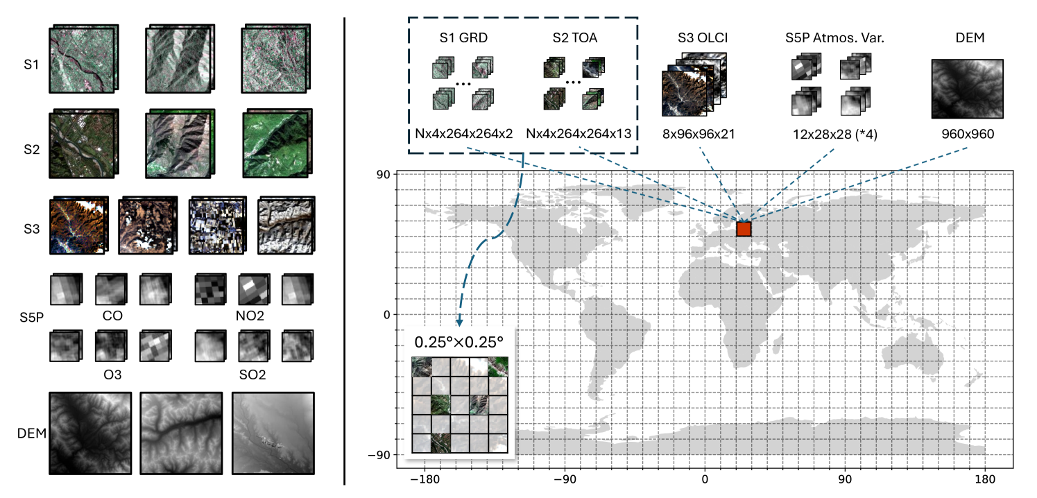
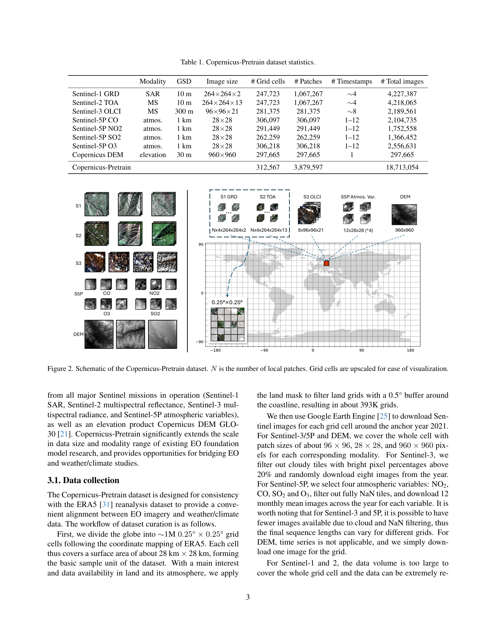
🔼 This figure illustrates the structure of the Copernicus-Pretrain dataset, a crucial component of the research. The dataset is composed of 0.25° × 0.25° grid cells covering the globe. Each grid cell contains multiple aligned images from various Copernicus Sentinel missions, including Sentinel-1 (SAR), Sentinel-2 (multispectral), Sentinel-3 (multispectral), Sentinel-5P (atmospheric), and a digital elevation model (DEM). The ‘N’ in the caption represents the number of image patches extracted from each grid cell, reflecting the varying resolutions and data density across different sensors. The grid cells are shown upscaled in the figure for better visualization, as the actual resolution of individual grid cells are much finer.
read the caption
Figure 2: Schematic of the Copernicus-Pretrain dataset. N𝑁Nitalic_N is the number of local patches. Grid cells are upscaled for ease of visualization.

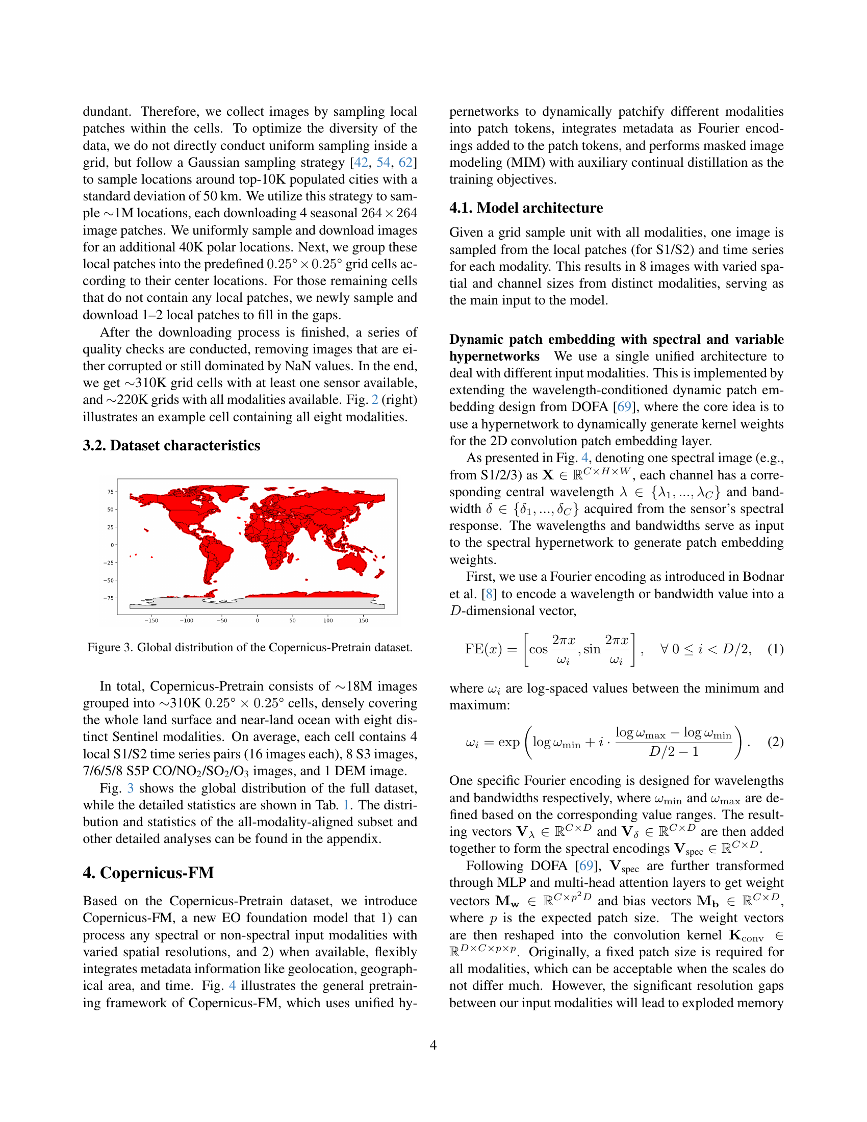
🔼 The figure displays a world map illustrating the global distribution of the Copernicus-Pretrain dataset. The color intensity indicates the density of data points, with darker regions representing areas with more data samples and lighter regions indicating areas with fewer samples. This visualization helps to understand the geographical coverage and data density of the dataset, which is crucial for evaluating the representativeness and potential biases of the training data used for developing Earth Observation foundation models.
read the caption
Figure 3: Global distribution of the Copernicus-Pretrain dataset.

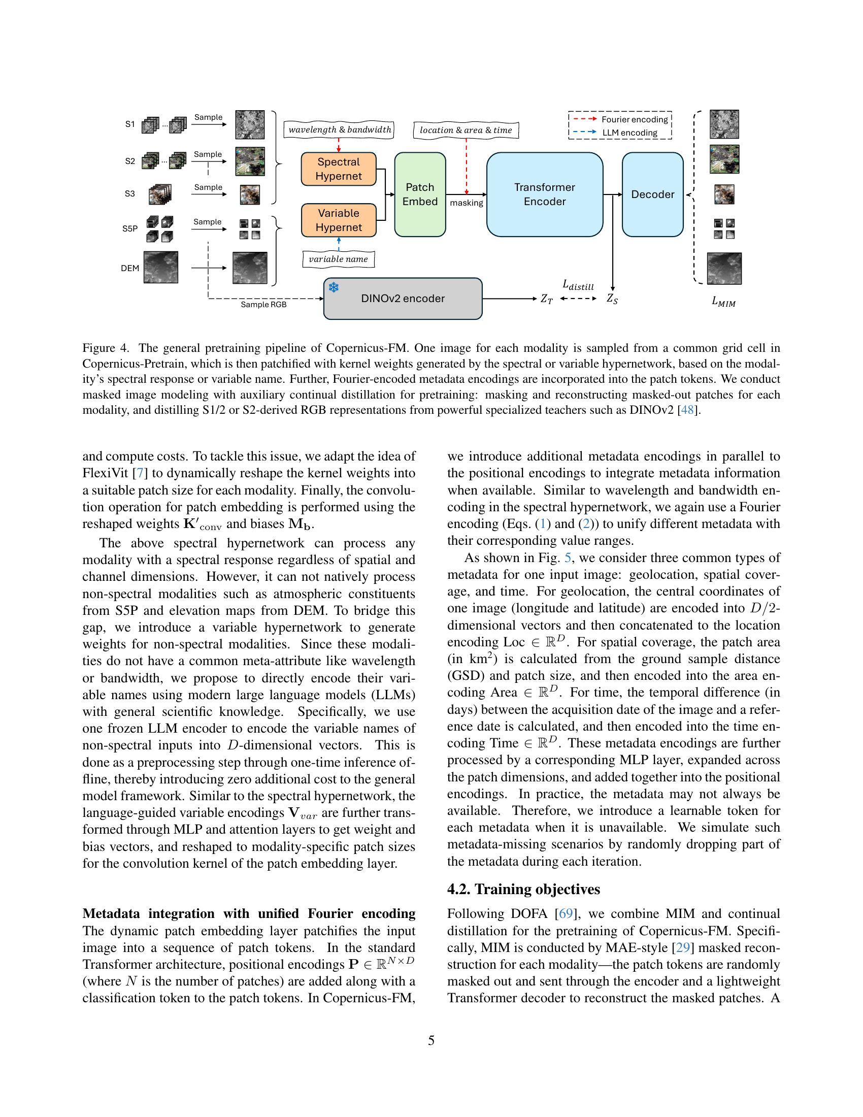
🔼 The figure illustrates the training process of the Copernicus-FM model. The model takes as input images from various Copernicus Sentinel missions (S1-S5P, DEM) sampled from a common grid cell. These images are first processed using dynamic hypernetworks to generate patch embeddings specific to the modality (spectral response for spectral data, or variable name for non-spectral data). Then, metadata (geolocation, area, and time) is incorporated using Fourier encodings. Masked Image Modeling (MIM) is employed, masking out parts of the input and training the model to reconstruct these masked parts. Simultaneously, auxiliary continual distillation is used by training the model to produce outputs similar to those from powerful teacher models such as DINOv2, trained on a subset of the data (RGB images derived from S1/S2).
read the caption
Figure 4: The general pretraining pipeline of Copernicus-FM. One image for each modality is sampled from a common grid cell in Copernicus-Pretrain, which is then patchified with kernel weights generated by the spectral or variable hypernetwork, based on the modality’s spectral response or variable name. Further, Fourier-encoded metadata encodings are incorporated into the patch tokens. We conduct masked image modeling with auxiliary continual distillation for pretraining: masking and reconstructing masked-out patches for each modality, and distilling S1/2 or S2-derived RGB representations from powerful specialized teachers such as DINOv2 [48].

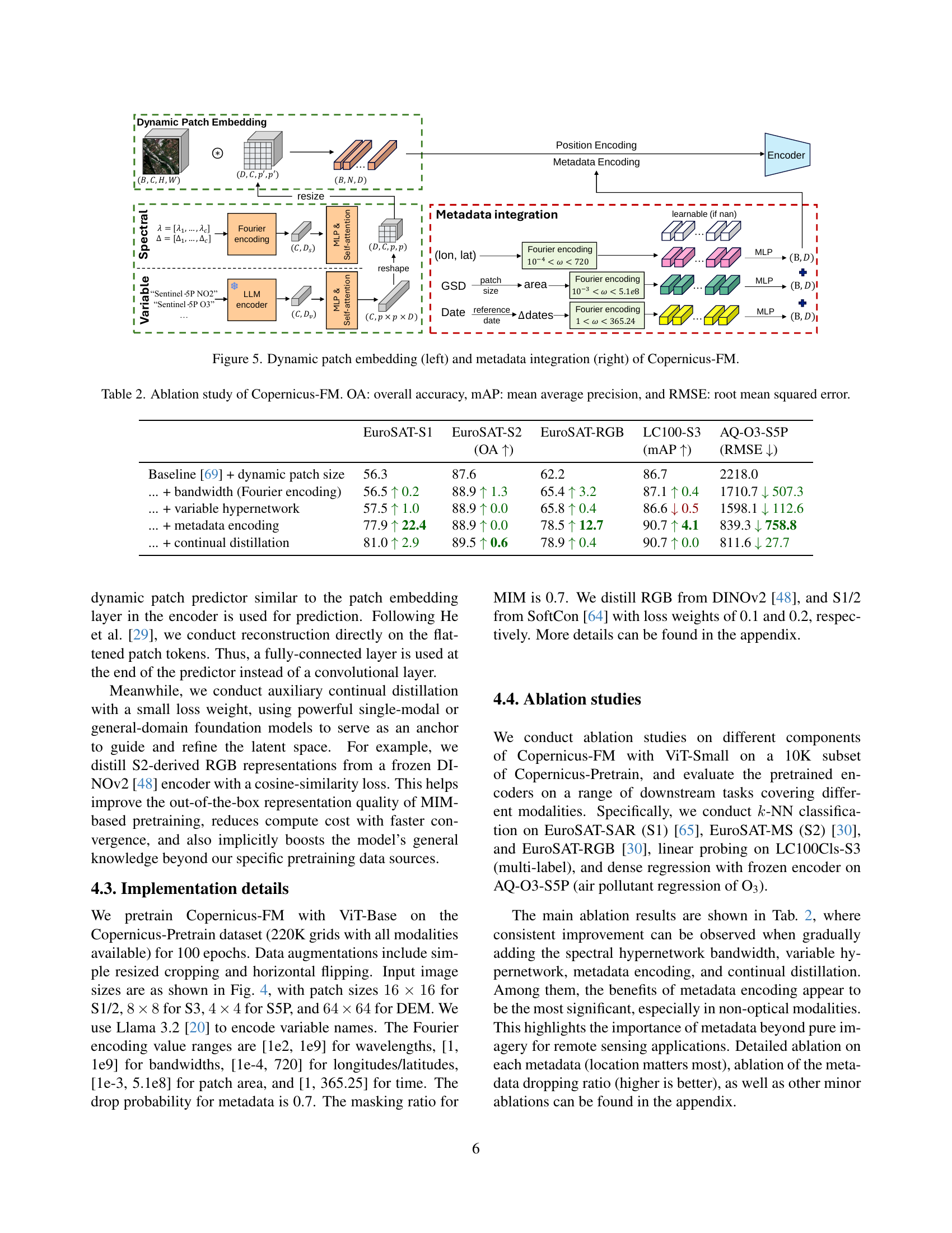
🔼 This figure illustrates the architecture of Copernicus-FM, specifically focusing on two key components: dynamic patch embedding and metadata integration. The left panel details how the model processes different image modalities (e.g., Sentinel-1 SAR, Sentinel-2 multispectral) with varying spatial resolutions. A hypernetwork dynamically generates kernel weights for a 2D convolution patch embedding layer, adapting to the unique spectral characteristics of each sensor. The right panel shows how metadata (geolocation, area, and time) is integrated into the model. Fourier encoding converts metadata into vectors that are added to patch tokens, providing additional context to the model during processing. The use of a unified architecture allows the model to handle various modalities and metadata in a flexible and scalable manner.
read the caption
Figure 5: Dynamic patch embedding (left) and metadata integration (right) of Copernicus-FM.

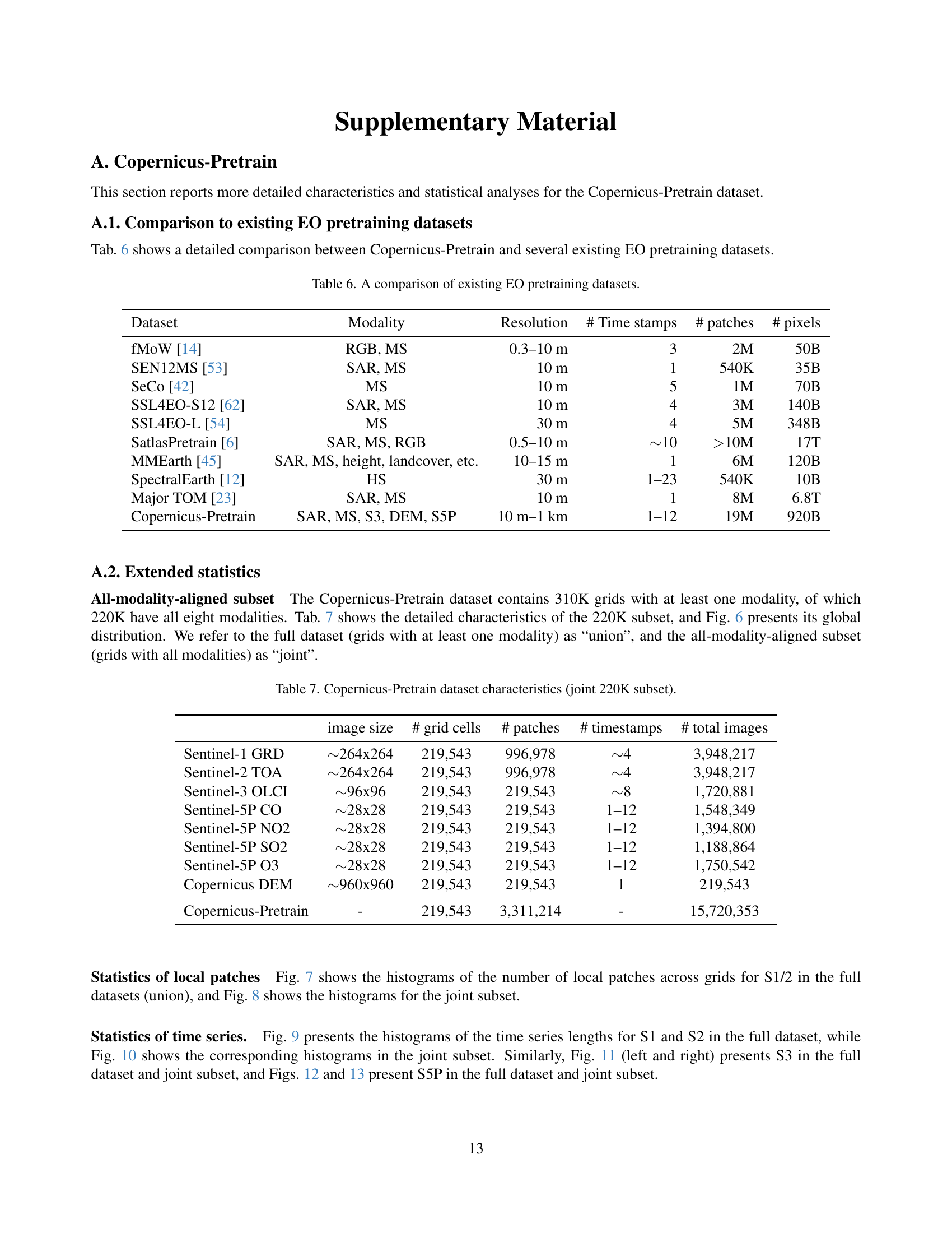
🔼 This figure shows a world map highlighting the geographical distribution of the Copernicus-Pretrain dataset’s ‘joint subset’. The ‘joint subset’ refers to the portion of the dataset containing complete data from all eight Sentinel missions and the Copernicus DEM GLO-30, ensuring comprehensive coverage across various modalities. The map uses color intensity to represent the density of grid cells included in the joint subset, providing a visual representation of data coverage.
read the caption
Figure 6: Global distribution of the joint subset of the Copernicus-Pretrain dataset.

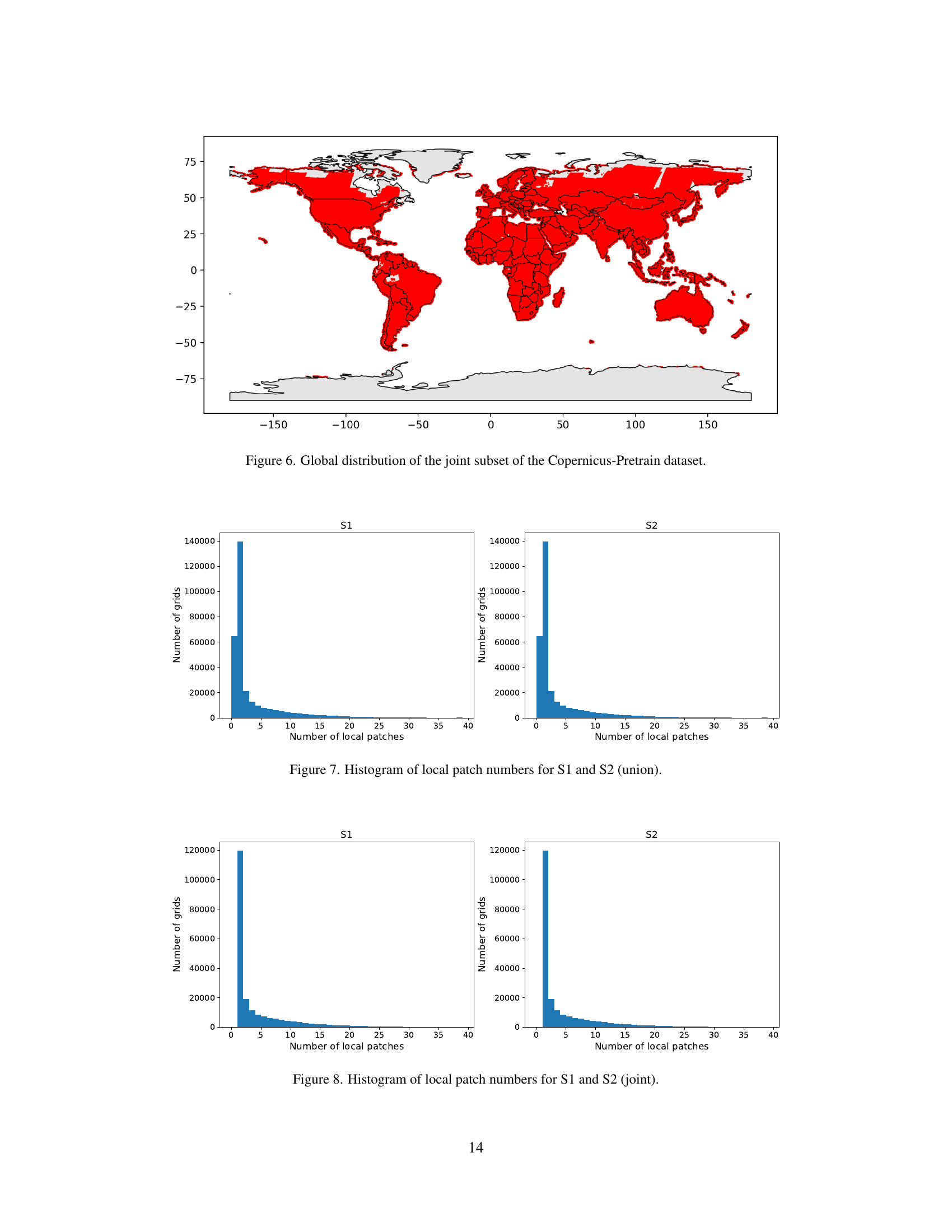
🔼 This figure shows two histograms, one each for Sentinel-1 (S1) and Sentinel-2 (S2) data. The histograms illustrate the distribution of the number of local image patches extracted from each of the 0.25° x 0.25° grid cells that compose the Copernicus-Pretrain dataset. The data shown represents the ‘union’ dataset, encompassing all grid cells with at least one sensor modality. The x-axis of each histogram shows the number of local patches and the y-axis shows the number of grids containing that many patches.
read the caption
Figure 7: Histogram of local patch numbers for S1 and S2 (union).

🔼 This histogram shows the distribution of the number of local image patches within each of the 0.25° x 0.25° grid cells for Sentinel-1 (S1) and Sentinel-2 (S2) data. The data used is the ‘joint’ subset of the Copernicus-Pretrain dataset, which means only grid cells containing data from all available sensor modalities are included. The x-axis represents the number of patches and the y-axis represents the number of grid cells with that many patches. The figure helps visualize the patch density variability across different regions in the dataset.
read the caption
Figure 8: Histogram of local patch numbers for S1 and S2 (joint).

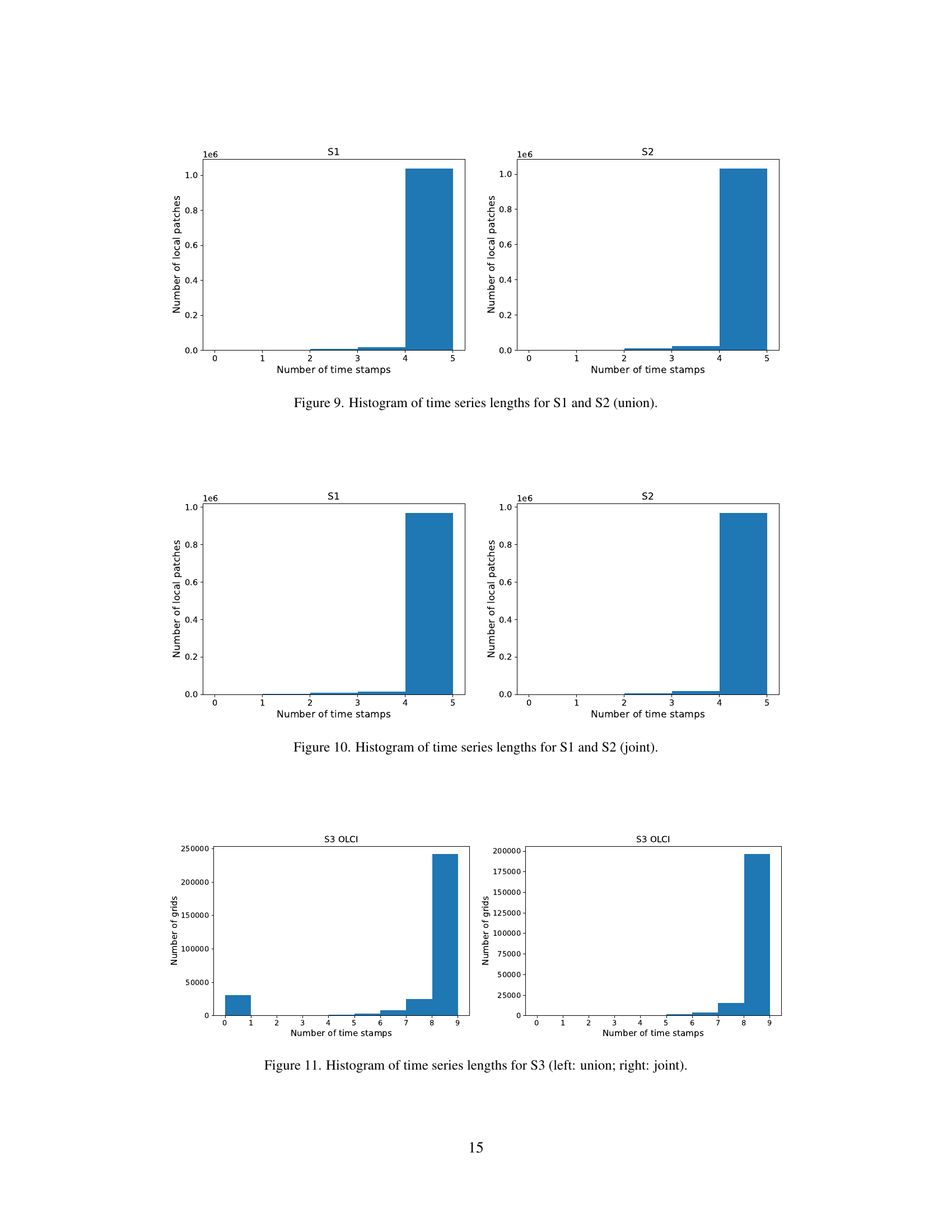
🔼 This figure shows the distribution of time series lengths for Sentinel-1 (S1) and Sentinel-2 (S2) data within the Copernicus-Pretrain dataset. The term ‘union’ signifies that this analysis includes all available data, regardless of whether a specific grid cell contains data from all sensor modalities. The histograms display the frequency of different time series lengths, providing insights into data availability and temporal coverage for both sensors.
read the caption
Figure 9: Histogram of time series lengths for S1 and S2 (union).

🔼 This figure shows two histograms illustrating the distribution of time series lengths for Sentinel-1 (S1) and Sentinel-2 (S2) data within the ‘joint’ subset of the Copernicus-Pretrain dataset. The ‘joint’ subset contains only grid cells where all eight data modalities are available. Each histogram displays the frequency of different time series lengths (number of observations over time), providing insights into the temporal coverage consistency for each sensor within this specific subset of the dataset.
read the caption
Figure 10: Histogram of time series lengths for S1 and S2 (joint).
🔼 This figure shows two histograms that visualize the distribution of time series lengths for Sentinel-3 data. The left histogram displays the data from the full Copernicus-Pretrain dataset (referred to as ‘union’), while the right histogram focuses on the subset of the data where all modalities are present (‘joint’). Each bar represents a specific number of time stamps, and the height of each bar indicates how many Sentinel-3 data samples have that number of time stamps in the dataset. Comparing the two histograms allows for an understanding of how data completeness and availability changes when considering the full dataset versus a more restricted dataset where all modalities are included.
read the caption
Figure 11: Histogram of time series lengths for S3 (left: union; right: joint).

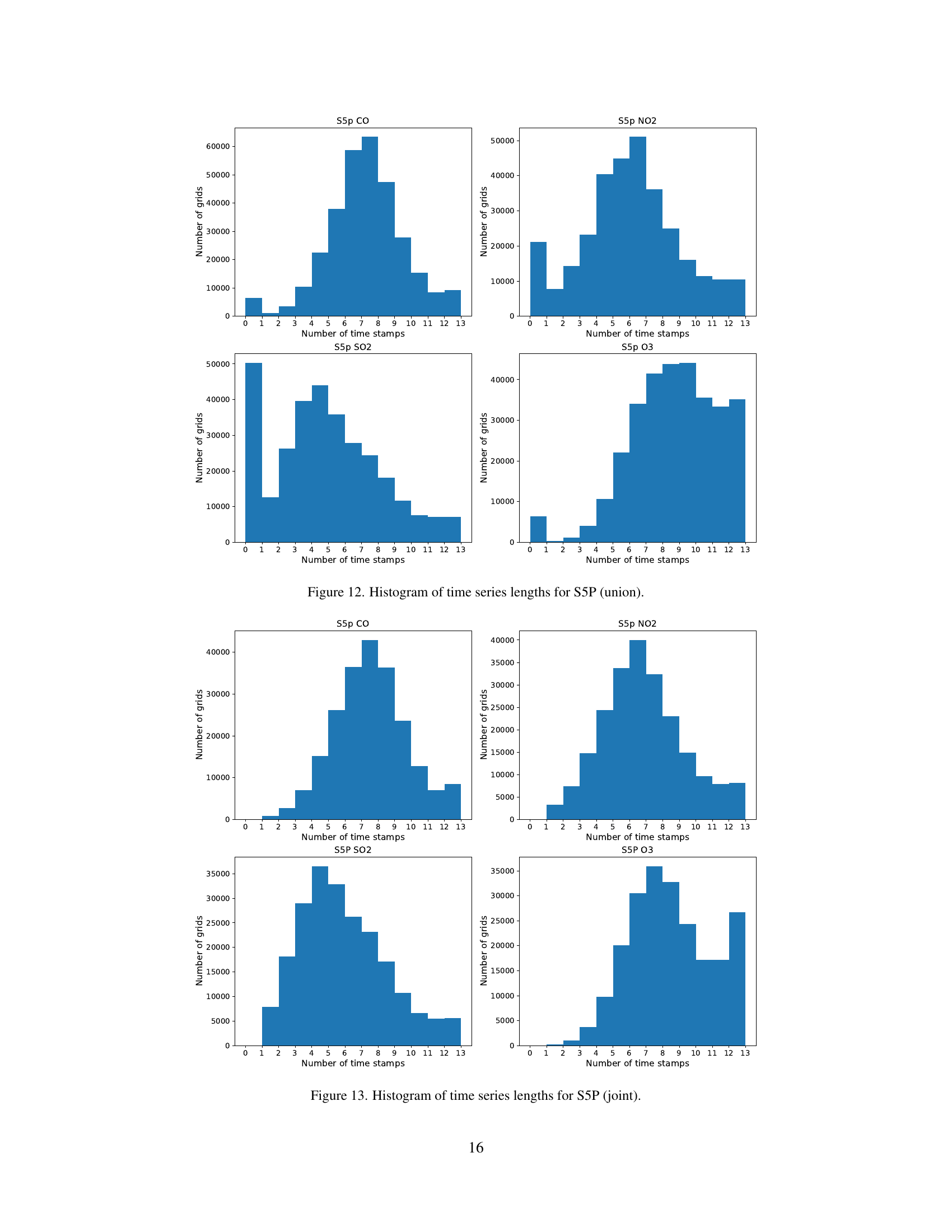
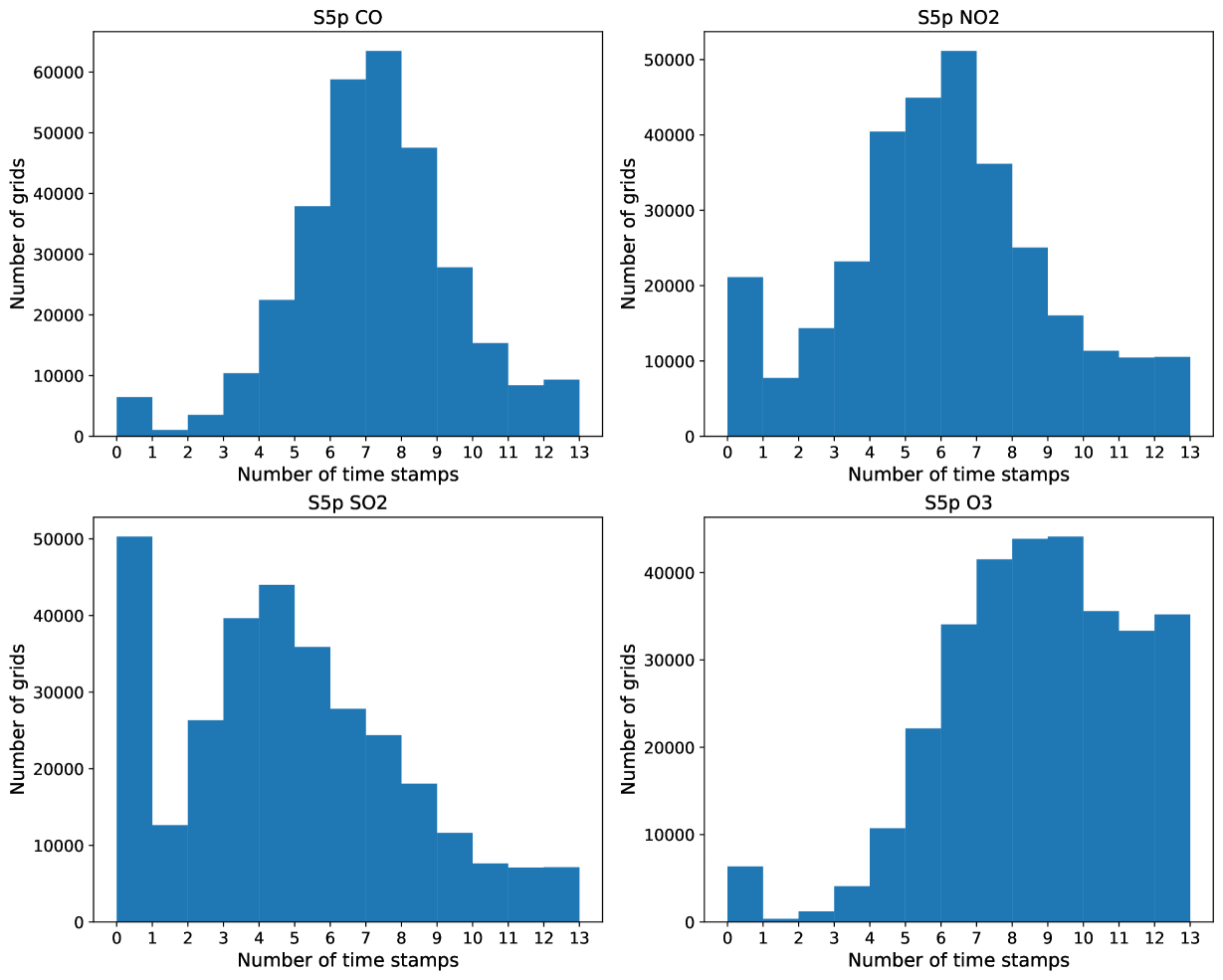
🔼 This figure shows the distribution of the number of time series observations available for each grid cell across various Sentinel-5P atmospheric variables (CO, NO2, SO2, and O3) in the Copernicus-Pretrain dataset. The dataset is called ‘union’ because it includes all grid cells with at least one available sensor modality. The x-axis represents the number of time stamps (months) and the y-axis represents the number of grid cells with that many observations. This visualization helps to understand the temporal coverage of the Sentinel-5P data within the Copernicus-Pretrain dataset and can inform the choices for model training.
read the caption
Figure 12: Histogram of time series lengths for S5P (union).

🔼 This figure presents histograms showing the distribution of time series lengths for each of the four atmospheric variables (CO, NO2, SO2, and O3) from the Sentinel-5P mission within the Copernicus-Pretrain dataset. The data shown represents only the subset of data where all eight modalities are available for each grid cell. The x-axis shows the number of time stamps and the y-axis shows the number of grid cells.
read the caption
Figure 13: Histogram of time series lengths for S5P (joint).

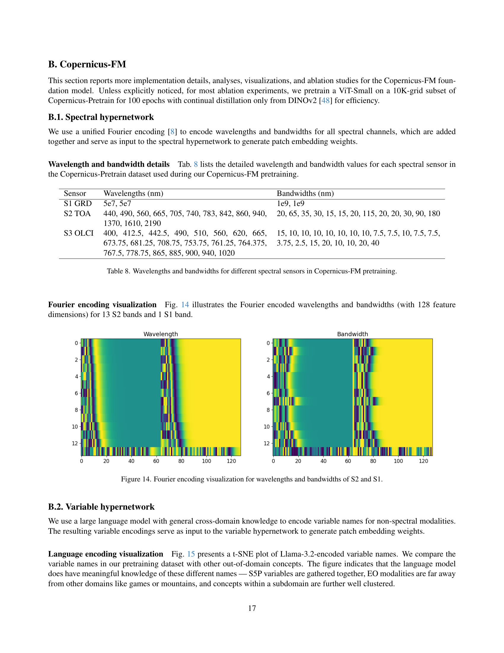
🔼 This figure visualizes the Fourier encoding of wavelengths and bandwidths used in the Copernicus-FM model for Sentinel-2 (S2) and Sentinel-1 (S1) data. The Fourier encoding transforms the wavelength and bandwidth values into higher-dimensional vectors which are used to dynamically generate the kernel weights for patch embedding within the model. The visualization helps illustrate how the model represents spectral information, enabling it to process different spectral sensors in a unified architecture.
read the caption
Figure 14: Fourier encoding visualization for wavelengths and bandwidths of S2 and S1.

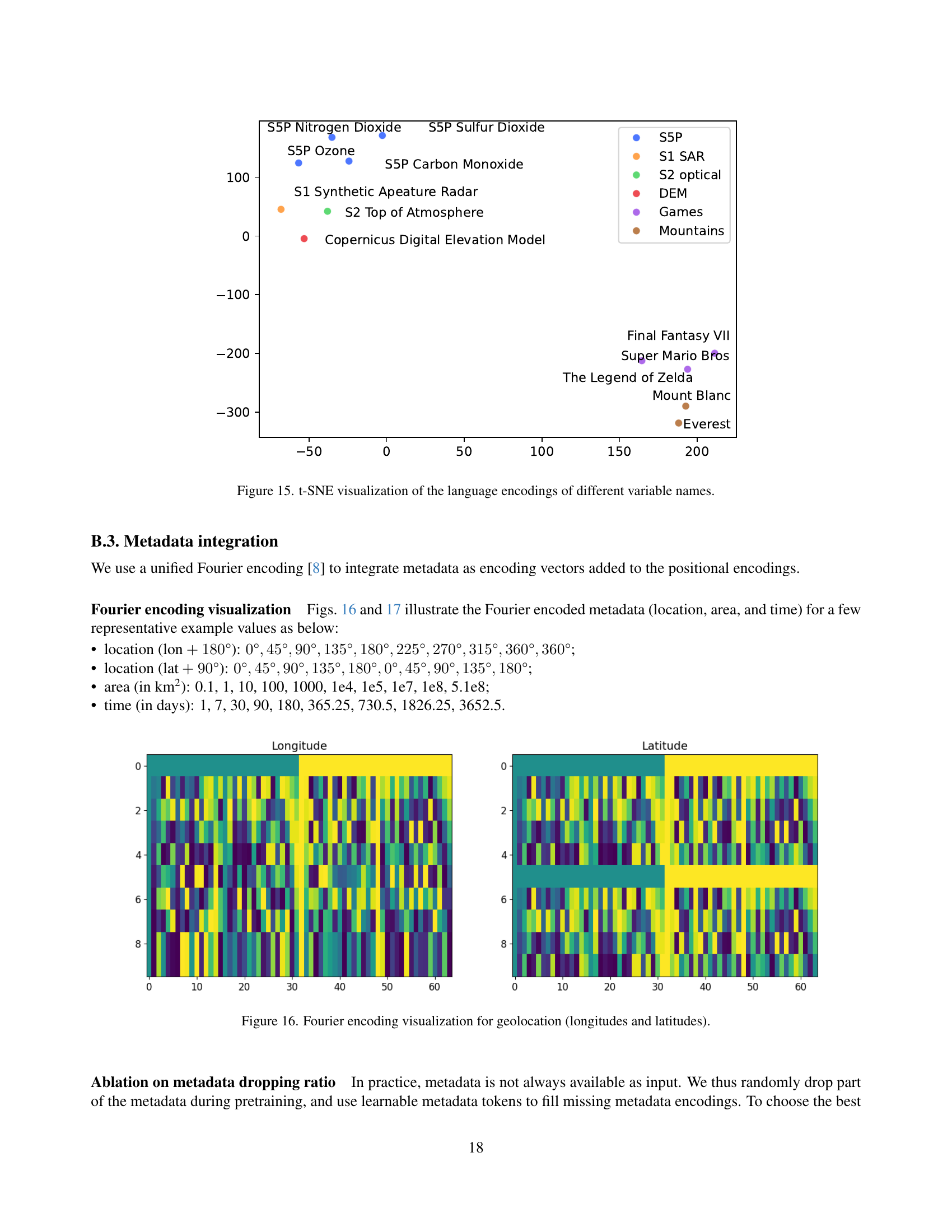
🔼 This t-SNE plot visualizes how a large language model (LLM) encodes different variable names used in the Copernicus-Pretrain dataset. The plot shows the relative distances between these encoded names in a lower-dimensional space. Variables with similar semantic meanings or relationships are clustered closer together, while dissimilar ones are further apart. This visualization demonstrates the LLM’s ability to capture the semantic relationships between the different variables, suggesting that it can effectively integrate metadata information into the Copernicus-FM model.
read the caption
Figure 15: t-SNE visualization of the language encodings of different variable names.

🔼 This figure visualizes the Fourier encoding applied to geolocation data (longitude and latitude). It shows how these geographical coordinates are transformed into a multi-dimensional vector representation using a Fourier encoding technique. The visualization helps illustrate how the encoding captures the spatial relationships and variations across different geographic locations, enabling the model to effectively learn representations sensitive to location.
read the caption
Figure 16: Fourier encoding visualization for geolocation (longitudes and latitudes).

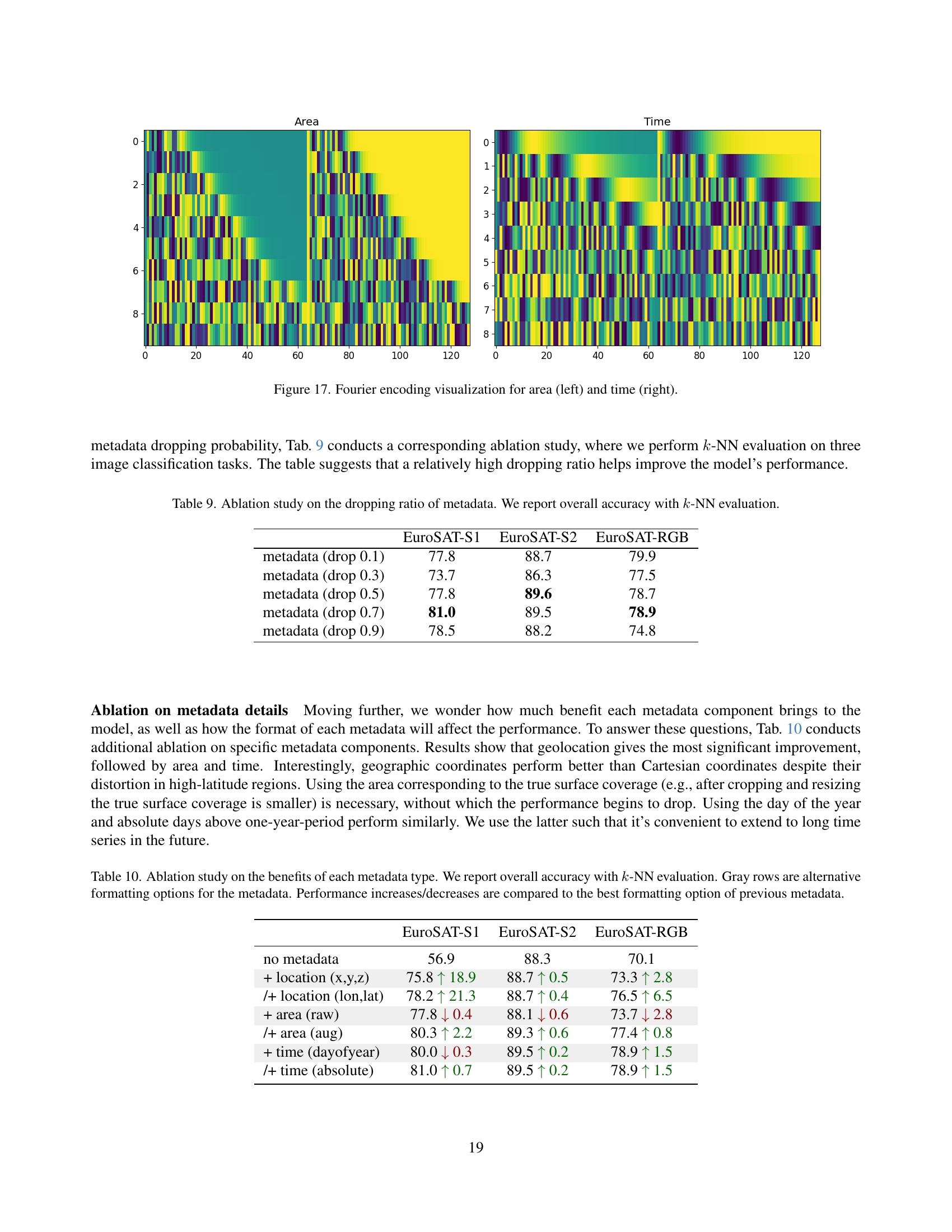
🔼 This figure visualizes the Fourier encoding of area and time metadata used in the Copernicus-FM model. The left panel shows the Fourier encoding for area, while the right panel displays the Fourier encoding for time. The color intensity represents the magnitude of the encoding vector, demonstrating how different values of area and time are represented within the model’s embedding space.
read the caption
Figure 17: Fourier encoding visualization for area (left) and time (right).

🔼 This figure shows example images and their corresponding cloud masks from the Copernicus-Bench Cloud-S2 dataset. The dataset is a subset of the CloudSEN12+ dataset and contains Sentinel-2 multispectral imagery with labels indicating cloud and cloud shadow. The images illustrate the diverse cloud cover conditions present in the dataset, including varying degrees of cloud cover and shadow.
read the caption
Figure 18: Copernicus-Bench-Cloud-S2.

🔼 This figure shows a comparison of the cloud segmentation results obtained from the Copernicus-Bench-Cloud-S3 dataset using two different approaches: a multi-class model and a binary classification model. The left side displays the results of the multi-class model, indicating multiple types of clouds and cloud-related features (e.g., clear, cloud-sure, cloud ambiguous, cloud shadow, snow-ice). The right side shows the results of the binary model, providing a simpler classification, distinguishing only between cloud/non-cloud. The images illustrate the difference in granularity and detail provided by the two models.
read the caption
Figure 19: Copernicus-Bench-Cloud-S3. Left: “multi-class” mode. Right: “binary” mode.

🔼 This figure displays sample images from the EuroSAT-S1 and EuroSAT-S2 datasets within the Copernicus-Bench benchmark. EuroSAT-S1 provides synthetic aperture radar (SAR) imagery, while EuroSAT-S2 offers multispectral imagery. The figure showcases the visual differences between these two data modalities for the same geographic location. This visual comparison is helpful in understanding the contrast between the information captured by different sensor types. Each image is labeled with the corresponding land cover class.
read the caption
Figure 20: Copernicus-Bench-EuroSAT-S1 and Copernicus-Bench-EuroSAT-S2.

🔼 This figure displays sample images from the BigEarthNet-S1 and BigEarthNet-S2 datasets, which are part of the Copernicus-Bench benchmark. BigEarthNet-S1 provides SAR imagery, while BigEarthNet-S2 offers multispectral data. The images are paired, showing the same geographical location but with different spectral properties. The corresponding ground truth labels for land cover classification are also shown, illustrating the variety of land cover types present in the datasets.
read the caption
Figure 21: Copernicus-Bench-BigEarth-S1 and Copernicus-Bench-BigEarth-S2.

🔼 This figure displays sample images from the Copernicus-Bench dataset, specifically focusing on the LC100Cls-S3 and LC100Seg-S3 datasets. These datasets utilize Sentinel-3 OLCI images and Copernicus Global Land Service (CGLS) land cover maps for classification and segmentation tasks. The images illustrate the multi-temporal aspect of the data, showing multiple images from a time series per location. The caption notes that by default, only one image per time series (the ‘static’ mode) is used for each location in the benchmark.
read the caption
Figure 22: Copernicus-Bench-LC100Cls-S3 and Copernicus-Bench-LC100Seg-S3. By default we pick one image per time series as “static” mode.
More on tables
| EuroSAT-S1 | EuroSAT-S2 | EuroSAT-RGB | LC100-S3 | AQ-O3-S5P | |
|---|---|---|---|---|---|
| (OA ) | (mAP ) | (RMSE ) | |||
| Baseline [69] + dynamic patch size | 56.3 | 87.6 | 62.2 | 86.7 | 2218.0 |
| … + bandwidth (Fourier encoding) | 56.5 0.2 | 88.9 1.3 | 65.4 3.2 | 87.1 0.4 | 1710.7 507.3 |
| … + variable hypernetwork | 57.5 1.0 | 88.9 0.0 | 65.8 0.4 | 86.6 0.5 | 1598.1 112.6 |
| … + metadata encoding | 77.9 22.4 | 88.9 0.0 | 78.5 12.7 | 90.7 4.1 | 839.3 758.8 |
| … + continual distillation | 81.0 2.9 | 89.5 0.6 | 78.9 0.4 | 90.7 0.0 | 811.6 27.7 |
🔼 This ablation study analyzes the impact of different components of the Copernicus-FM model on its performance across four benchmark datasets. The study evaluates the overall accuracy (OA), mean average precision (mAP), and root mean squared error (RMSE), depending on the specific dataset and task. The components analyzed include the use of dynamic patch sizes, Fourier encoding for bandwidths, a variable hypernetwork, metadata encoding, and continual distillation.
read the caption
Table 2: Ablation study of Copernicus-FM. OA: overall accuracy, mAP: mean average precision, and RMSE: root mean squared error.
| Dataset | Modality | Resolution | # Time stamps | # patches | # pixels |
|---|---|---|---|---|---|
| fMoW [14] | RGB, MS | 0.3–10 m | 3 | 2M | 50B |
| SEN12MS [53] | SAR, MS | 10 m | 1 | 540K | 35B |
| SeCo [42] | MS | 10 m | 5 | 1M | 70B |
| SSL4EO-S12 [62] | SAR, MS | 10 m | 4 | 3M | 140B |
| SSL4EO-L [54] | MS | 30 m | 4 | 5M | 348B |
| SatlasPretrain [6] | SAR, MS, RGB | 0.5–10 m | 10 | 10M | 17T |
| MMEarth [45] | SAR, MS, height, landcover, etc. | 10–15 m | 1 | 6M | 120B |
| SpectralEarth [12] | HS | 30 m | 1–23 | 540K | 10B |
| Major TOM [23] | SAR, MS | 10 m | 1 | 8M | 6.8T |
| Copernicus-Pretrain | SAR, MS, S3, DEM, S5P | 10 m–1 km | 1–12 | 19M | 920B |
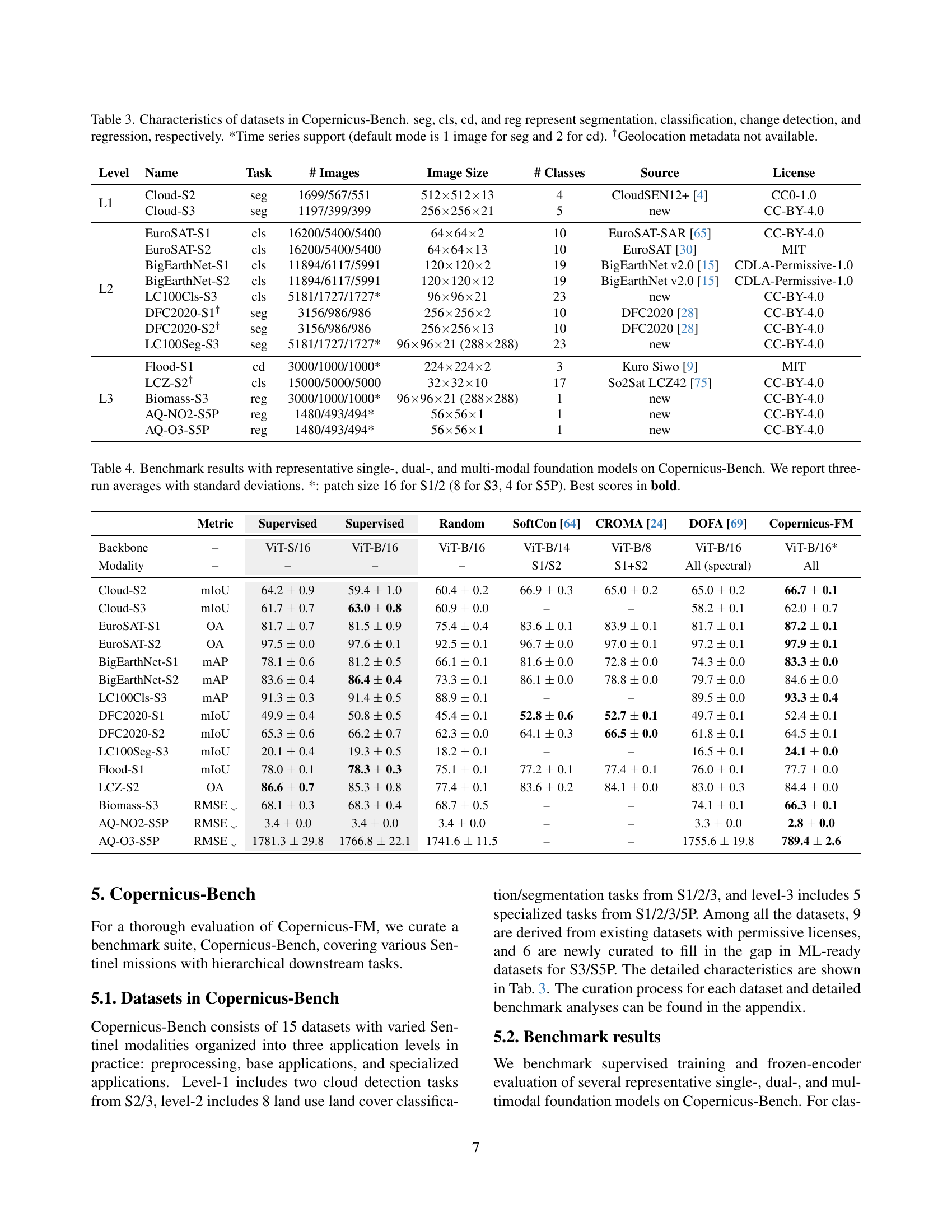
🔼 Table 3 details the datasets used in the Copernicus-Bench benchmark. It lists each dataset’s name, task type (segmentation, classification, change detection, or regression), number of images, image dimensions, number of classes, data source, and license. It also notes whether the dataset supports time series data (with the default number of images per time series indicated) and whether geolocation metadata is available.
read the caption
Table 3: Characteristics of datasets in Copernicus-Bench. seg, cls, cd, and reg represent segmentation, classification, change detection, and regression, respectively. *Time series support (default mode is 1 image for seg and 2 for cd). †Geolocation metadata not available.
| image size | # grid cells | # patches | # timestamps | # total images | |
|---|---|---|---|---|---|
| Sentinel-1 GRD | 264x264 | 219,543 | 996,978 | 4 | 3,948,217 |
| Sentinel-2 TOA | 264x264 | 219,543 | 996,978 | 4 | 3,948,217 |
| Sentinel-3 OLCI | 96x96 | 219,543 | 219,543 | 8 | 1,720,881 |
| Sentinel-5P CO | 28x28 | 219,543 | 219,543 | 1–12 | 1,548,349 |
| Sentinel-5P NO2 | 28x28 | 219,543 | 219,543 | 1–12 | 1,394,800 |
| Sentinel-5P SO2 | 28x28 | 219,543 | 219,543 | 1–12 | 1,188,864 |
| Sentinel-5P O3 | 28x28 | 219,543 | 219,543 | 1–12 | 1,750,542 |
| Copernicus DEM | 960x960 | 219,543 | 219,543 | 1 | 219,543 |
| Copernicus-Pretrain | - | 219,543 | 3,311,214 | - | 15,720,353 |
🔼 This table presents a quantitative comparison of various foundation models’ performance on the Copernicus-Bench benchmark. The benchmark consists of 15 diverse Earth observation tasks, spanning different Sentinel missions and complexities (pre-processing, basic applications, specialized applications). The models tested include single-modal, dual-modal, and multi-modal approaches. Performance is evaluated using metrics appropriate for each task (e.g., mean Intersection over Union (mIoU) for segmentation, overall accuracy (OA) for classification, Root Mean Squared Error (RMSE) for regression). The table shows the mean and standard deviation of three independent runs for each model and task, allowing for statistical significance testing. Note that certain tasks used different patch sizes for different sensors (S1, S2, S3, and S5P). The best performance for each task is highlighted in bold.
read the caption
Table 4: Benchmark results with representative single-, dual-, and multi-modal foundation models on Copernicus-Bench. We report three-run averages with standard deviations. *: patch size 16 for S1/2 (8 for S3, 4 for S5P). Best scores in bold.
| Sensor | Wavelengths (nm) | Bandwidths (nm) |
|---|---|---|
| S1 GRD | 5e7, 5e7 | 1e9, 1e9 |
| S2 TOA | 440, 490, 560, 665, 705, 740, 783, 842, 860, 940, 1370, 1610, 2190 | 20, 65, 35, 30, 15, 15, 20, 115, 20, 20, 30, 90, 180 |
| S3 OLCI | 400, 412.5, 442.5, 490, 510, 560, 620, 665, 673.75, 681.25, 708.75, 753.75, 761.25, 764.375, 767.5, 778.75, 865, 885, 900, 940, 1020 | 15, 10, 10, 10, 10, 10, 10, 10, 7.5, 7.5, 10, 7.5, 7.5, 3.75, 2.5, 15, 20, 10, 10, 20, 40 |
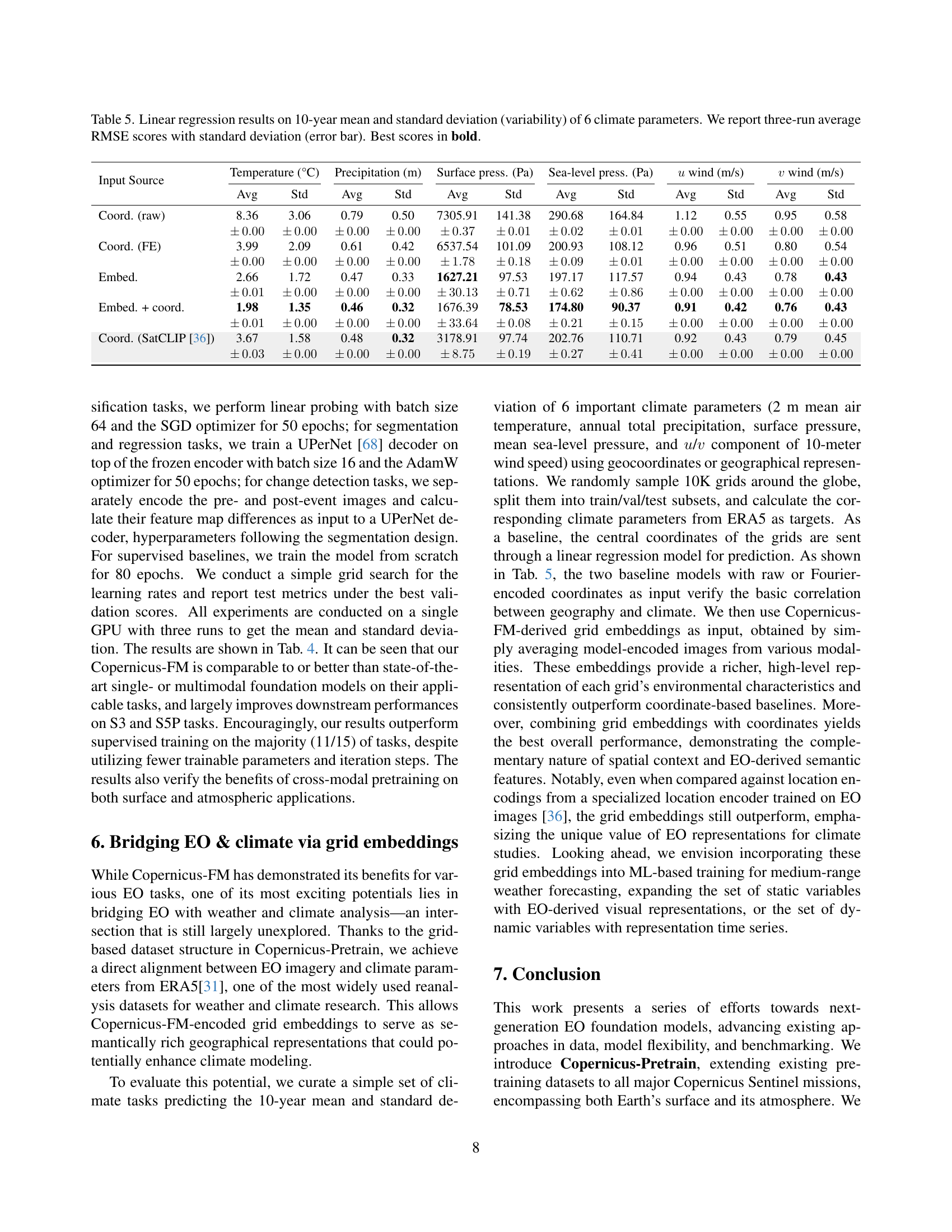
🔼 This table presents the results of linear regression models used to predict six different climate parameters (temperature, precipitation, surface pressure, sea-level pressure, and u/v wind components). The models used different input data: raw coordinates, coordinates combined with embeddings from the Copernicus-FM model, and embeddings alone. The table shows the average RMSE and standard deviation (error bar) across three runs for each model and input combination. Lower RMSE values indicate better prediction accuracy. The best performing model for each climate parameter is highlighted in bold.
read the caption
Table 5: Linear regression results on 10-year mean and standard deviation (variability) of 6 climate parameters. We report three-run average RMSE scores with standard deviation (error bar). Best scores in bold.
| EuroSAT-S1 | EuroSAT-S2 | EuroSAT-RGB | |
|---|---|---|---|
| metadata (drop 0.1) | 77.8 | 88.7 | 79.9 |
| metadata (drop 0.3) | 73.7 | 86.3 | 77.5 |
| metadata (drop 0.5) | 77.8 | 89.6 | 78.7 |
| metadata (drop 0.7) | 81.0 | 89.5 | 78.9 |
| metadata (drop 0.9) | 78.5 | 88.2 | 74.8 |
🔼 This table compares several existing Earth Observation (EO) pretraining datasets, highlighting key differences in terms of the sensor modalities used (e.g., RGB, multispectral, SAR), the spatial resolution of the imagery, the temporal coverage (number of time stamps), the total number of patches or images in the dataset, and the overall size of the dataset (in pixels or bytes). It provides a useful overview of the scale and scope of various publicly available EO datasets used for training foundation models.
read the caption
Table 6: A comparison of existing EO pretraining datasets.
| EuroSAT-S1 | EuroSAT-S2 | EuroSAT-RGB | |
|---|---|---|---|
| no metadata | 56.9 | 88.3 | 70.1 |
| + location (x,y,z) | 75.8 18.9 | 88.7 0.5 | 73.3 2.8 |
| /+ location (lon,lat) | 78.2 21.3 | 88.7 0.4 | 76.5 6.5 |
| + area (raw) | 77.8 0.4 | 88.1 0.6 | 73.7 2.8 |
| /+ area (aug) | 80.3 2.2 | 89.3 0.6 | 77.4 0.8 |
| + time (dayofyear) | 80.0 0.3 | 89.5 0.2 | 78.9 1.5 |
| /+ time (absolute) | 81.0 0.7 | 89.5 0.2 | 78.9 1.5 |
🔼 This table presents a detailed breakdown of the Copernicus-Pretrain dataset focusing on the subset containing all eight modalities (220K grid cells). It provides the image size, the number of grid cells, patches, timestamps, and the total number of images for each of the eight Sentinel missions included. The table offers a precise view of the dataset’s composition and data volume for researchers seeking to understand the dataset’s scale and diversity.
read the caption
Table 7: Copernicus-Pretrain dataset characteristics (joint 220K subset).
| # tasks | task types | modalities | resolution | task range | |
|---|---|---|---|---|---|
| SustainBench [72] | 15 | cls, seg, reg | RGB, MS | 0.6–30 m | surface |
| GEO-Bench [37] | 12 | cls, seg | RGB, MS, HS, SAR | 0.1–15 m | surface |
| FoMo-Bench [10] | 16 | cls, seg, obj | RGB, MS, HS, SAR | 0.01–60 m | surface |
| PhilEO Bench [22] | 3 | seg, reg | MS | 10 m | surface |
| Copernicus-Bench (ours) | 15 | cls, seg, reg, cd | MS, SAR, atmos. var. | 10–1000 m | surface, atmosphere |
🔼 This table lists the specific wavelengths and their corresponding bandwidths used for each of the spectral sensors included in the Copernicus-FM pretraining dataset. This detailed spectral information is crucial for understanding how the model processes different spectral bands, allowing for a more comprehensive understanding of the model’s architecture and functionality.
read the caption
Table 8: Wavelengths and bandwidths for different spectral sensors in Copernicus-FM pretraining.
Full paper#