TL;DR#
Large Vision-Language Models (LVLMs) often struggle with long-tail (LT) problems, where some data categories are over-represented while others are scarce. Current methods focus on traditional VLM architectures and specific tasks, leaving the broader exploration of LVLMs and general tasks under-explored. A key issue identified here is that head concepts are overly represented while tail concepts are under-represented, leading to imbalanced model performance.
To address this, the paper introduces an Adaptive Data Refinement Framework (ADR), consisting of Data Rebalancing (DR) and Data Synthesis (DS) stages. DR adaptively rebalances redundant data based on entity distributions, while DS uses Denoising Diffusion Probabilistic Models to supplement under-represented portions. The results show that ADR effectively improves the performance of LLaVA 1.5 across eleven benchmarks by 4.36% without increasing the data volume.
Key Takeaways#
Why does it matter?#
This paper is important for researchers due to its in-depth analysis of LT problems in LVLMs and the introduction of ADR, a novel framework, easily integrated into open-source LVLMs. ADR’s dual approach of rebalancing and synthesizing data addresses unique challenges. The significant performance gains without increasing data volume make it highly relevant for advancing more robust and balanced multimodal AI systems.
Visual Insights#

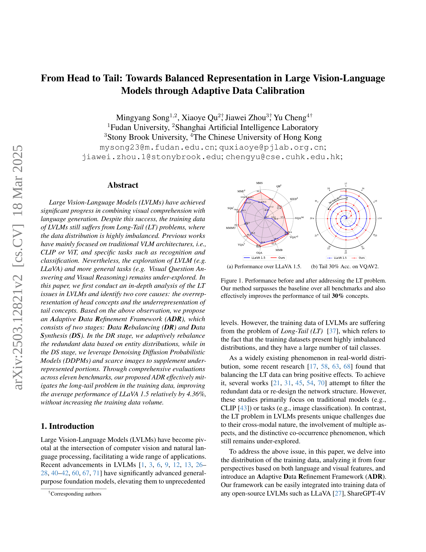
🔼 This figure shows the performance comparison between the original LLaVA 1.5 model and the model enhanced with the proposed Adaptive Data Refinement (ADR) framework. The (a) subplot displays a radar chart comparing the performance across eleven benchmarks. Each axis represents a benchmark, and the distance from the center represents the performance score, showing that the ADR-enhanced model consistently outperforms LLaVA 1.5 across all benchmarks. The (b) subplot focuses specifically on the accuracy of the tail 30% of concepts within the VQAV2 benchmark, further illustrating the improved performance of the ADR-enhanced model in handling the long-tail distribution problem.
read the caption
((a))
| Data | Level | thres | % E | % DI |
|---|---|---|---|---|
| LLaVA [27] | Tok | 120 | 98.7 | 10.0 |
| Obj | 304 | 98.0 | 10.0 | |
| Co | 24 | 92.7 | 25.0 | |
| Int | 4895 | 99.6 | 10.0 | |
| Avg. | - | - | 97.25 | 13.75 |
🔼 This table presents the relative amount of tail data (data representing less frequent entities) remaining after a reverse indexing process was applied to the LLaVA 1.5 instruction tuning dataset. The analysis considers four different perspectives: Tokens (individual words), Objects (visual concepts), Co-occurrences (relationships between objects), and Interrogations (types of questions). For each perspective, it shows the percentage of tail entities (%E) and the percentage of data instances associated with these tail entities (%DI). A higher percentage of data instances associated with a smaller percentage of entities indicates a long-tail problem, where a few frequent entities dominate the data while many infrequent entities are underrepresented.
read the caption
Table 1: Relative data volume of tail data after reverse indexing. “Tok”, “Obj”, “Co”, and “Int” represent Token, Object, Co-occurrence, and Interrogation, respectively. %E denotes the percentage of tail entities, while %DI indicates the percentage of tail data instances.
In-depth insights#
LVLM Long-Tail#
The Long-Tail (LT) problem in Large Vision-Language Models (LVLMs) highlights a critical challenge: data imbalance. Traditional methods often focus on CLIP or ViT architectures and specific tasks like classification. However, LVLMs, exemplified by LLaVA, performing general tasks like visual question answering require deeper exploration. This imbalance manifests as an overrepresentation of common concepts and an underrepresentation of rarer ones, skewing model learning. This analysis shows many open-source LVLMs need improvement. The unique co-occurrence and cross-modal nature of LVLMs pose distinct challenges compared to traditional models. A potential solution involves Adaptive Data Refinement (ADR). ADR integrates data rebalancing and synthesis which helps to mitigate the issues of over represented and under represented data. A comprehensive analysis of tokens, objects, co-occurrences, and interrogations provides insights into the causes and propose solutions to resolve the LT issues.
Adaptive Refine#
The concept of an ‘Adaptive Refinement’ process, likely within a model like an LVLM, strongly suggests a methodology for iteratively improving performance by adjusting data. This could involve techniques like re-weighting data based on difficulty or importance, focusing on areas where the model struggles. Data augmentation or synthesis, generating new examples to address imbalances, could also fall under adaptive refinement. Calibration, is a key component, it could also be dynamically adjusting model parameters to better align with the true data distribution. This approach indicates a commitment to robustness and generalization, addressing potential biases or weaknesses in the initial training. The adaptation iteratively refines the model’s ability to extract information.
LT Problem Causes#
The research paper identifies two primary causes for the Long-Tail (LT) problem in Large Vision-Language Models (LVLMs). First, there is an overrepresentation of head concepts in the training data. This means that common objects, entities, or relationships are disproportionately present. Second, there is an underrepresentation of tail concepts. Rare objects, unusual relationships, or subtle visual cues are scarce in the data. This imbalance leads the LVLMs to perform well on frequent concepts but struggle with infrequent ones. Addressing these causes is crucial for improving the robustness and generalization ability of LVLMs.
Synthesizing Data#
Data synthesis emerges as a crucial strategy to tackle the challenge of scarce data, especially in vision-language models. This involves creating new, realistic data points to augment existing datasets, thereby improving model generalization and robustness. Effective synthesis techniques leverage methods such as generative adversarial networks and variational autoencoders, carefully crafting images and text to mimic real-world distributions. The goal is to populate underrepresented regions of the data space, reducing bias and enhancing performance on tail concepts that are often poorly captured in imbalanced datasets. A careful balance must be struck to avoid introducing artifacts or unrealistic patterns that could negatively affect model learning.
ADR Superiority#
The concept of ‘ADR Superiority’ suggests an innovative approach to enhancing model performance, likely through adaptive data refinement. This implies superiority over existing methods due to ADR’s capability to dynamically adjust data based on underlying patterns, addressing imbalances and biases. It highlights the significance of data-centric refinement, where superior outcomes aren’t achieved by tweaking the model but by optimizing the training data itself. ADR’s superiority could stem from its ability to automate intricate data adjustments, reducing manual intervention. The ‘superiority’ further emphasizes the efficiency and efficacy of ADR in diverse scenarios.
More visual insights#
More on figures

🔼 This figure shows the accuracy of the model on the tail 30% of the data in VQAV2. The baseline LLaVA 1.5 model and the improved model using the proposed ADR method are compared. The chart displays a radar plot showing performance across multiple aspects of the task. The ADR method demonstrates significantly improved accuracy for the tail 30% concepts.
read the caption
((b))

🔼 This figure displays a comparison of performance on various benchmarks before and after addressing the long-tail (LT) problem in Large Vision-Language Models (LVLMs). The left subplot (a) shows the performance improvement of the proposed method (Ours) compared to the LLaVA 1.5 baseline across different benchmarks. The right subplot (b) focuses specifically on the accuracy achieved on the tail 30% of concepts within the VQAV2 benchmark, highlighting that the proposed method significantly enhances the performance on the tail concepts.
read the caption
Figure 1: Performance before and after addressing the LT problem. Our method surpasses the baseline over all benchmarks and also effectively improves the performance of tail 30% concepts.

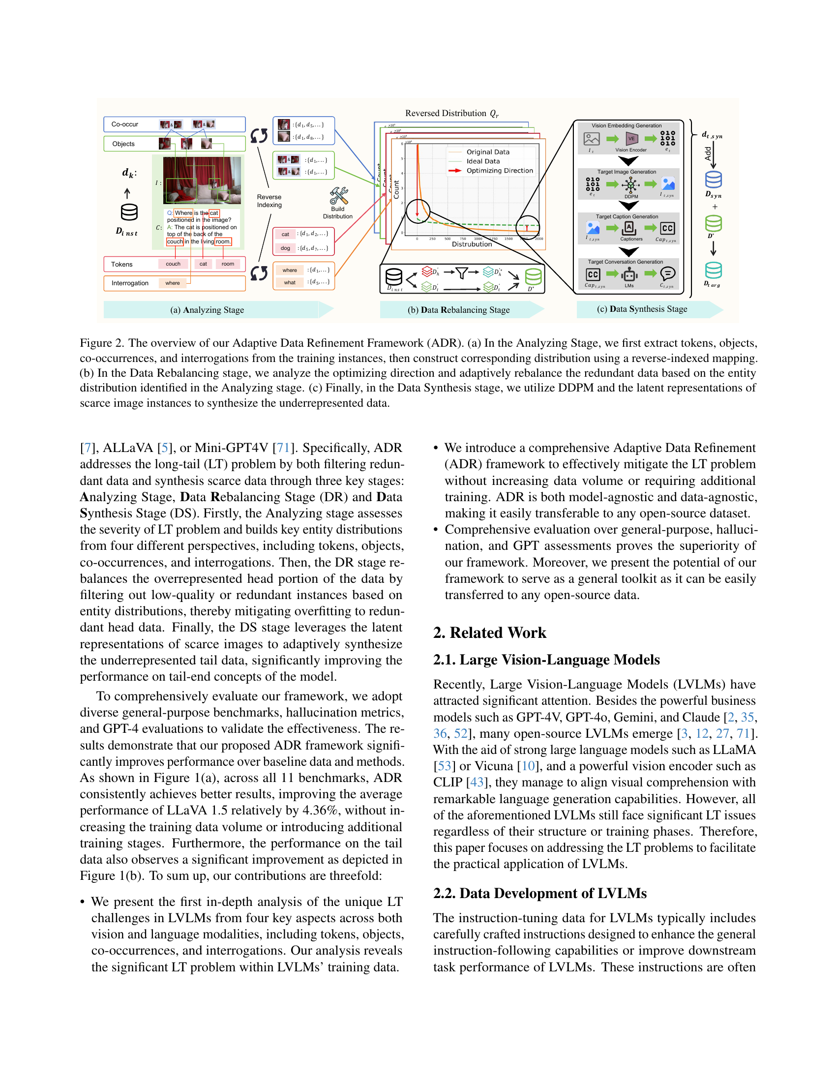
🔼 Figure 2 illustrates the Adaptive Data Refinement Framework (ADR), a three-stage process to address data imbalance in large vision-language models. Stage (a) Analyzing, extracts key features (tokens, objects, co-occurrences, and interrogations) from the training data and generates their distributions. Stage (b) Data Rebalancing, uses this information to identify and remove redundant data while retaining the data with under-represented entities. Finally, stage (c) Data Synthesis, leverages diffusion probabilistic models and limited data to generate synthetic data for underrepresented categories.
read the caption
Figure 2: The overview of our Adaptive Data Refinement Framework (ADR). (a) In the Analyzing Stage, we first extract tokens, objects, co-occurrences, and interrogations from the training instances, then construct corresponding distribution using a reverse-indexed mapping. (b) In the Data Rebalancing stage, we analyze the optimizing direction and adaptively rebalance the redundant data based on the entity distribution identified in the Analyzing stage. (c) Finally, in the Data Synthesis stage, we utilize DDPM and the latent representations of scarce image instances to synthesize the underrepresented data.

🔼 The figure shows the performance comparison between LLaVA 1.5 and the proposed method on eleven benchmarks. Subfigure (a) displays the average performance improvement across all benchmarks, showing that the proposed method outperforms LLaVA 1.5. Subfigure (b) focuses on the accuracy achieved on the tail 30% of concepts within the VQAV2 benchmark, demonstrating a significant improvement by the proposed method compared to LLaVA 1.5. This visualization highlights the effectiveness of the proposed method in addressing the long-tail problem in large vision-language models.
read the caption
((a))

🔼 This figure shows the accuracy of the model on the tail 30% of concepts in the VQAV2 benchmark. It compares the performance of the original LLaVA 1.5 model to the model enhanced with the proposed ADR (Adaptive Data Refinement) framework. The chart visually demonstrates that the ADR-improved model significantly outperforms the baseline model on the more challenging, less frequent concepts (tail data).
read the caption
((b))

🔼 This figure shows the Data Synthesis stage of the Adaptive Data Refinement Framework (ADR). It illustrates the process of generating underrepresented tail data using Denoising Diffusion Probabilistic Models (DDPMs). Specifically, it demonstrates how latent representations of scarce images are leveraged to synthesize new images and captions representing underrepresented concepts, thereby mitigating the long-tail problem in the training data.
read the caption
((c))

🔼 This figure shows the object-level word distribution in LLaVA’s instruction tuning dataset. It illustrates the long-tail distribution problem in the training data, where a small number of objects are overrepresented (head), while a large number of objects are underrepresented (tail). This imbalance can negatively affect the performance of the model on the underrepresented tail concepts.
read the caption
((d))

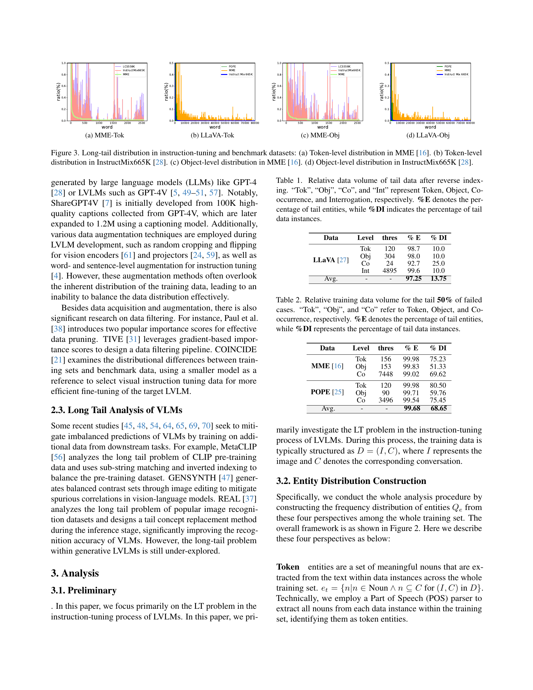
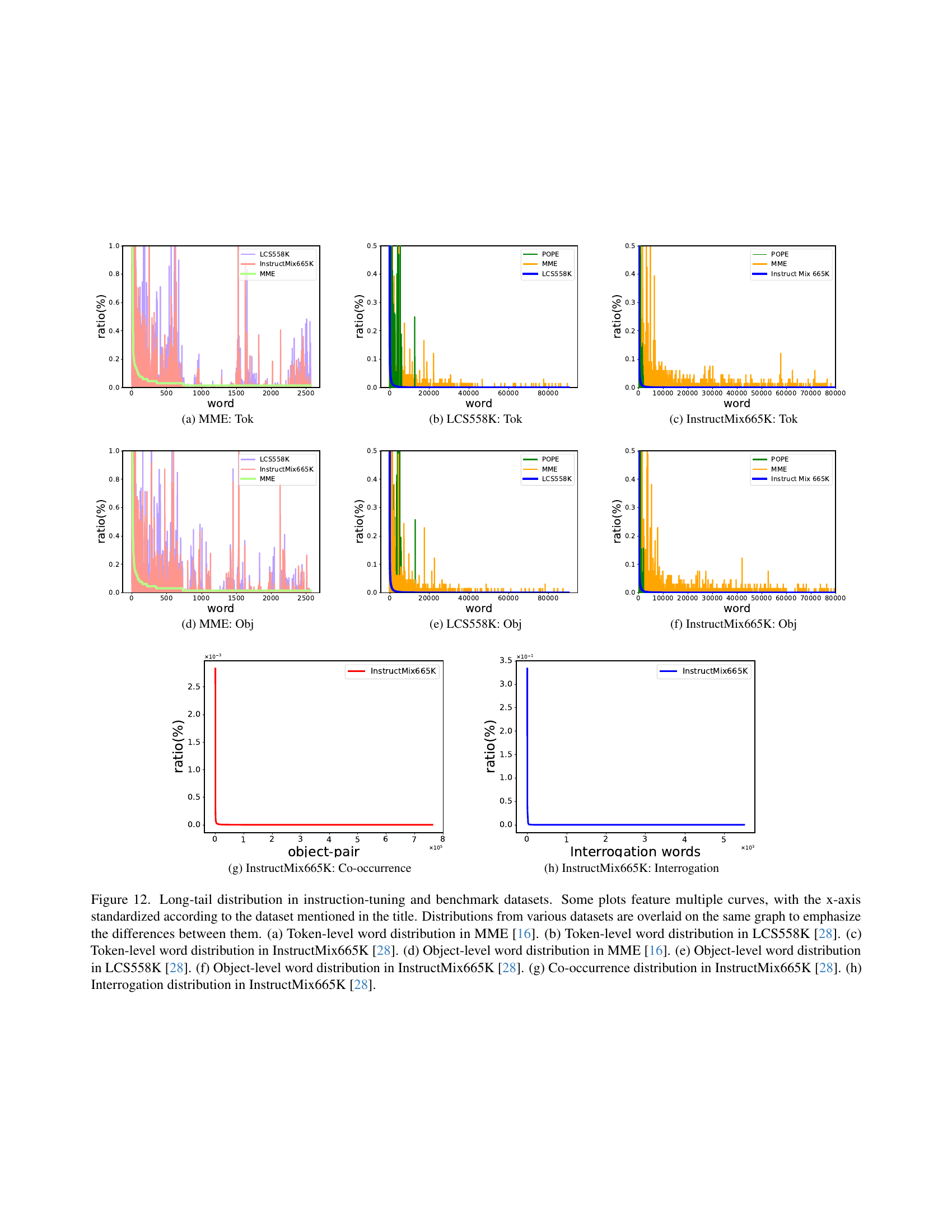
🔼 This figure visualizes the long-tail distributions in instruction-tuning and benchmark datasets, specifically focusing on token-level and object-level distributions. Subfigures (a) and (c) show the distributions in the MME dataset, while subfigures (b) and (d) show those in the InstructMix665K dataset. The long tail is a common problem in datasets where some categories have far more examples than others. These plots help illustrate the severity of this class imbalance, indicating the challenge for models trained on such data.
read the caption
Figure 3: Long-tail distribution in instruction-tuning and benchmark datasets: (a) Token-level distribution in MME [16]. (b) Token-level distribution in InstructMix665K [28]. (c) Object-level distribution in MME [16]. (d) Object-level distribution in InstructMix665K [28].

🔼 This figure shows the performance comparison between LLaVA 1.5 and the proposed method (Ours) on various vision-language benchmarks. Subfigure (a) presents the performance comparison across different benchmarks, demonstrating that the proposed method outperforms LLaVA 1.5 consistently and significantly improves the average performance. Subfigure (b) focuses on the accuracy on the tail 30% of concepts in the VQAV2 benchmark, illustrating the effectiveness of the proposed method in mitigating the long-tail problem and improving the performance on less frequent concepts.
read the caption
((a))

🔼 This figure shows the accuracy of the model on the tail 30% of the data in the VQAV2 benchmark. It compares the performance of the original LLaVA 1.5 model against the improved model after applying the Adaptive Data Refinement (ADR) framework. The chart visually demonstrates the significant improvement achieved by ADR in handling the long-tail problem. The increased accuracy on the tail data indicates that the ADR method effectively addresses the imbalance in the training data and enhances the model’s overall performance.
read the caption
((b))

🔼 This figure shows the Data Synthesis stage of the Adaptive Data Refinement Framework (ADR). It illustrates the process of using Denoising Diffusion Probabilistic Models (DDPMs) and latent representations of scarce images to supplement under-represented portions of the training data. The diagram details how the system leverages vision encoders, captioners, and language models (LMs) to synthesize both visual and textual information, generating new image-caption pairs for underrepresented tail concepts.
read the caption
((c))

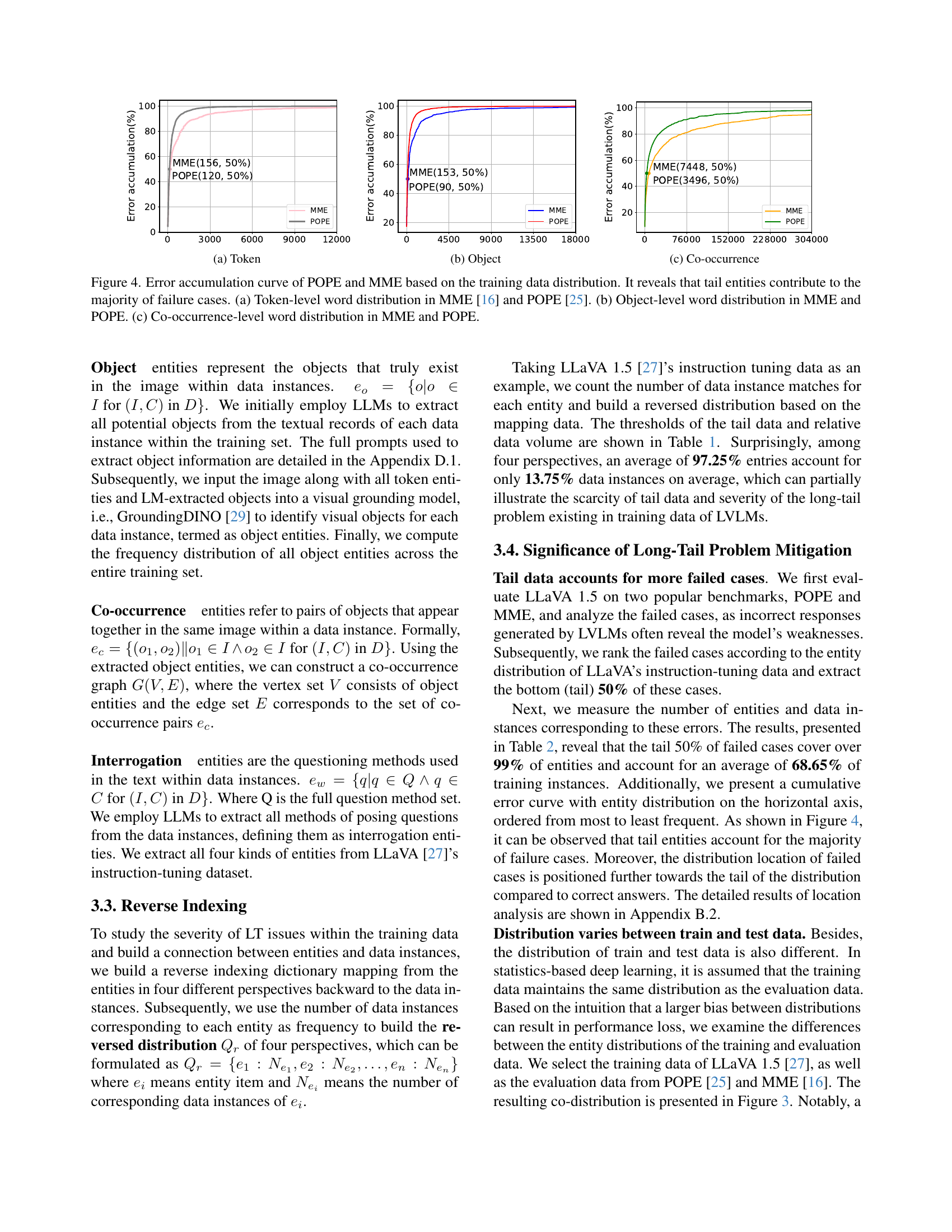
🔼 Figure 4 displays error accumulation curves for the POPE and MME datasets, illustrating the disproportionate contribution of tail entities to prediction errors. The curves show that while a small percentage of frequent entities account for many correct predictions, a large portion of less frequent tail entities are associated with the majority of failures. Panel (a) shows the analysis at the token level, panel (b) at the object level, and panel (c) at the co-occurrence level, offering a multi-faceted understanding of how long-tail effects manifest across different granularities of analysis in the datasets.
read the caption
Figure 4: Error accumulation curve of POPE and MME based on the training data distribution. It reveals that tail entities contribute to the majority of failure cases. (a) Token-level word distribution in MME [16] and POPE [25]. (b) Object-level word distribution in MME and POPE. (c) Co-occurrence-level word distribution in MME and POPE.
🔼 This ablation study investigates the impact of different combinations of data rebalancing methods on the overall performance of a large vision-language model (LLaVA 1.5). The study uses four perspectives to rebalance the data: Token, Object, Co-occurrence, and Interrogation (represented by T, O, C, and W respectively). Each bar in the graph shows the average performance across multiple benchmarks when using various combinations of these rebalancing techniques. The blue dashed line serves as the baseline performance of LLaVA 1.5 without any data rebalancing. This allows for a direct comparison and visualization of the effectiveness of different rebalancing strategies.
read the caption
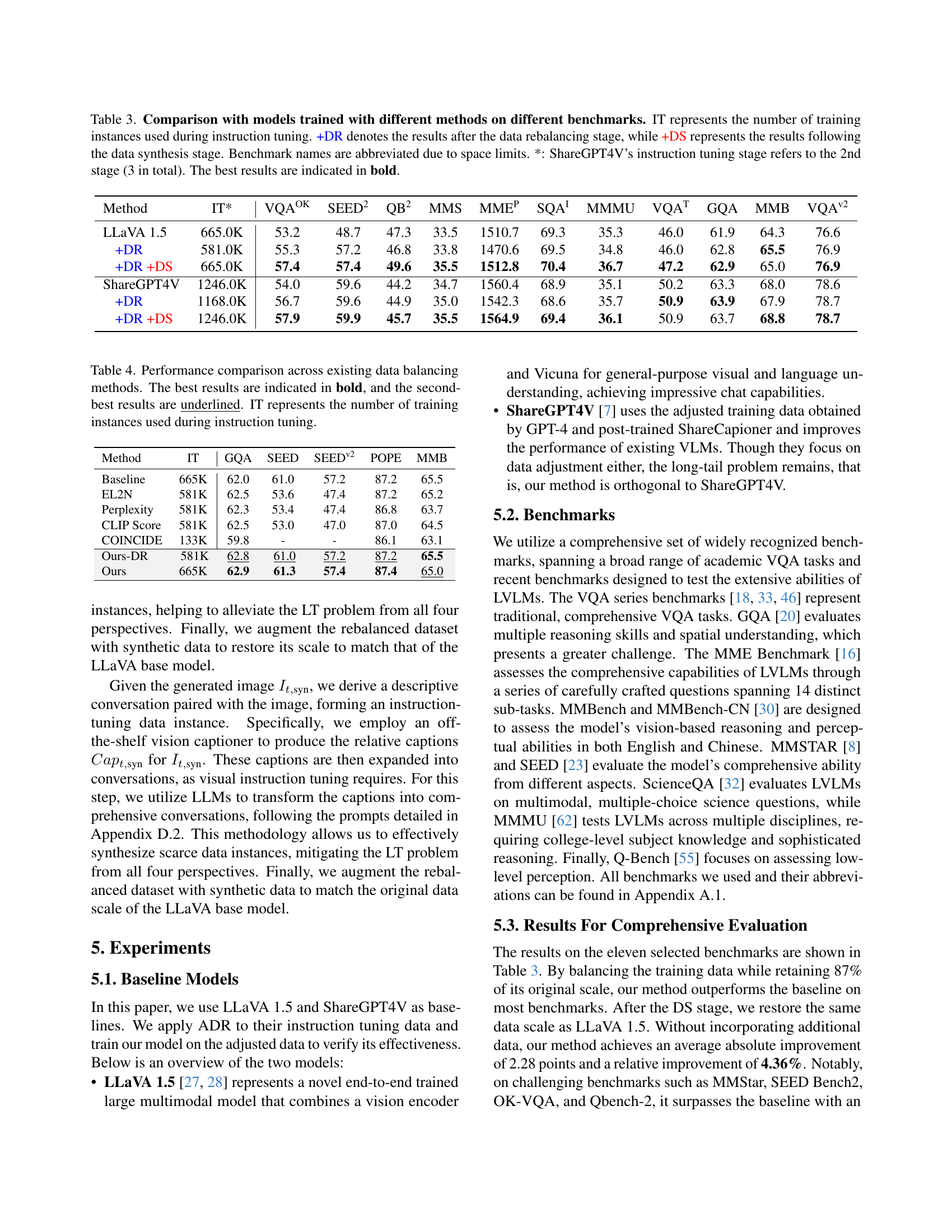
Figure 5: Ablation study on data rebalancing combinations. T, O, C, and W refer to Token, Object, Co-occurrence, and Interrogation respectively. The values displayed in the graph represent average scores across a variety of comprehensive benchmarks. The blue dashed line indicates the baseline performance of LLaVA 1.5.

🔼 This ablation study investigates the impact of different data rebalancing and synthesis methods on the overall performance of a large vision-language model (LLaVA 1.5). The x-axis represents various combinations of techniques (explained in Section 6.2), and the y-axis shows the average performance across multiple comprehensive benchmarks. The blue dashed line indicates the baseline performance of the LLaVA 1.5 model without any data augmentation or rebalancing. The results illustrate which combination of data rebalancing and synthesis methods yields the best performance improvement on average.
read the caption
Figure 6: Ablation study on data rebalancing synthesis methods. The meaning of abbrs occurred here is explained in Section 6.2. The values displayed in the graph represent average scores across a variety of comprehensive benchmarks. The blue dashed line indicates the baseline performance of LLaVA 1.5.

🔼 This figure presents a qualitative comparison of LLaVA 1.5 (baseline) and LLaVA with the proposed ADR method in answering tail questions (questions related to less frequent concepts). A tail example is provided to highlight the difference in performance. The example demonstrates that LLaVA 1.5 struggles with the tail question and fails to provide a correct answer, while LLaVA with ADR successfully answers the same question. This visually demonstrates the improvement in handling under-represented data achieved through the use of the ADR framework.
read the caption
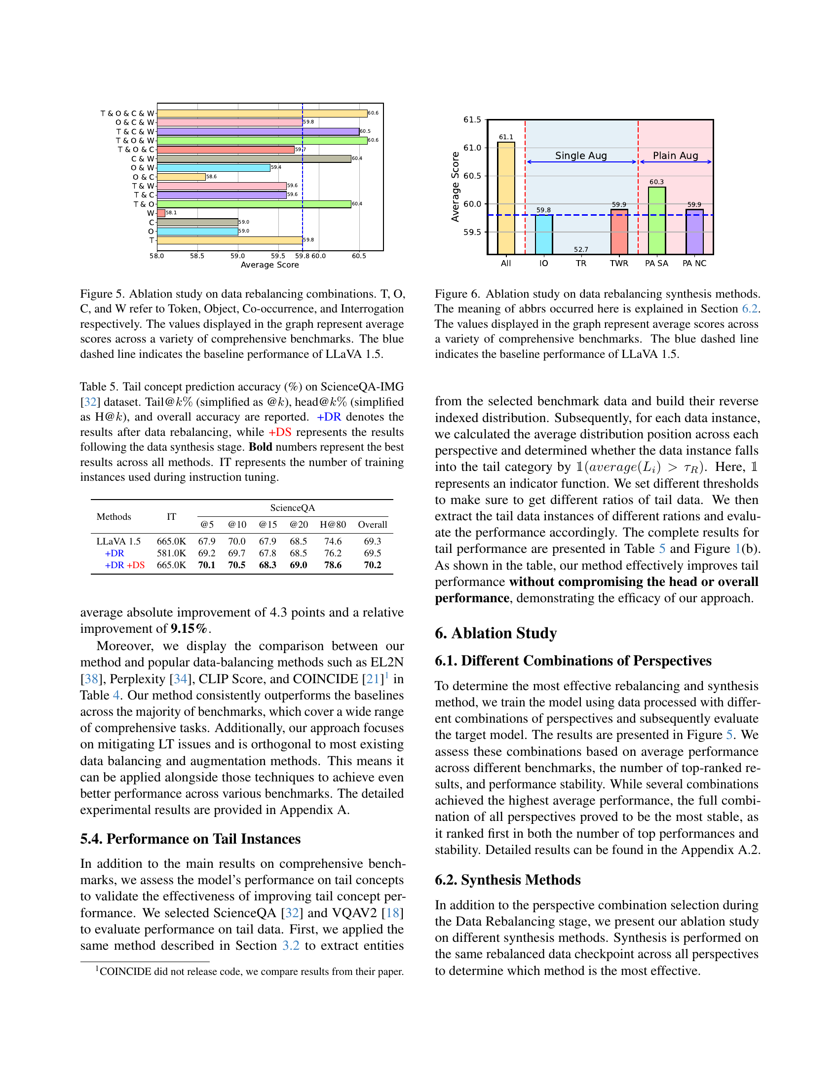
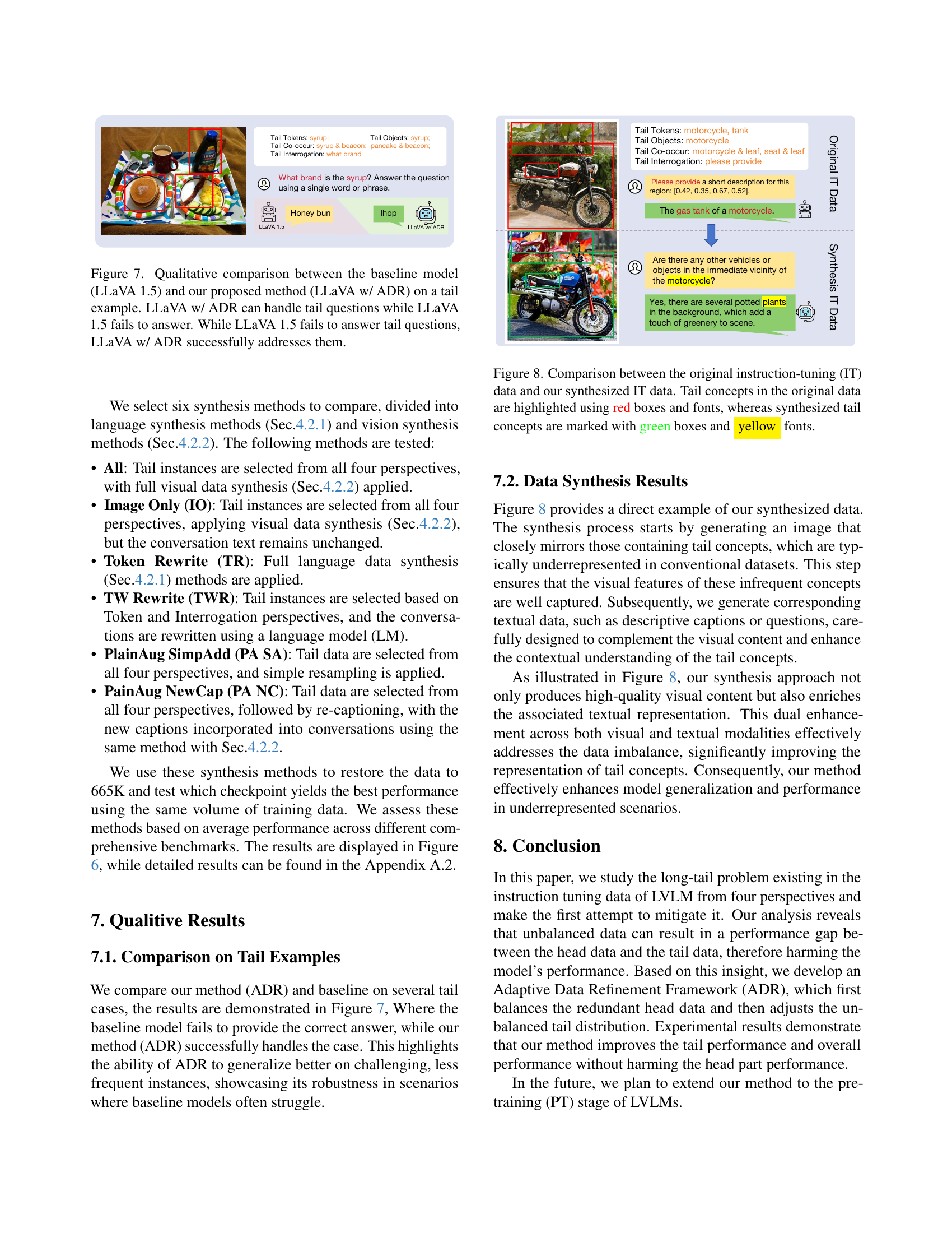
Figure 7: Qualitative comparison between the baseline model (LLaVA 1.5) and our proposed method (LLaVA w/ ADR) on a tail example. LLaVA w/ ADR can handle tail questions while LLaVA 1.5 fails to answer. While LLaVA 1.5 fails to answer tail questions, LLaVA w/ ADR successfully addresses them.

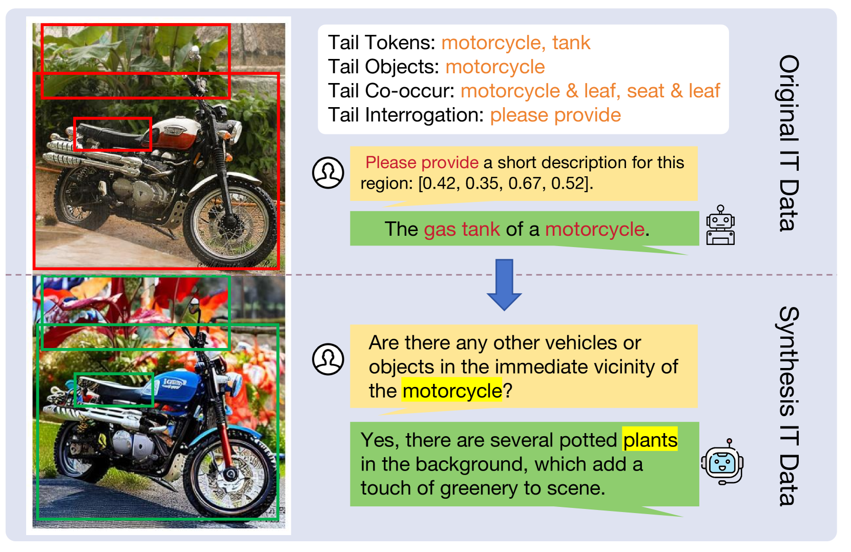
🔼 Figure 8 visualizes a comparison between the original instruction-tuning dataset and the data synthesized by the proposed method. The image showcases examples from both datasets, highlighting tail concepts (under-represented concepts in the original dataset). Tail concepts in the original data are marked with red boxes and red font, while the synthesized tail concepts are marked with green boxes and yellow font. This allows for a direct visual comparison of the original data’s limitations and how the proposed method addresses these limitations by supplementing the dataset with synthesized examples of tail concepts.
read the caption
Figure 8: Comparison between the original instruction-tuning (IT) data and our synthesized IT data. Tail concepts in the original data are highlighted using red boxes and fonts, whereas synthesized tail concepts are marked with green boxes and yellow fonts.

🔼 A photograph depicting a bear calmly situated next to a rock wall. The setting appears natural and serene, suggesting a wildlife environment. The bear’s posture is relaxed, indicating a peaceful moment.
read the caption
((a)) A bear resting peacefully beside a rock wall.

🔼 A cell phone screen displays a cartoon princess. The image is used as an example in the paper to illustrate a challenge in a Vision-Language Model (VLM). The model is shown to have difficulty in identifying details in images containing underrepresented concepts or objects (referred to as ’tail concepts’ in the paper). The example highlights the need for the Adaptive Data Refinement Framework (ADR) that the paper proposes.
read the caption
((b)) A cell phone displaying a cartoon princess on its screen.

🔼 The image shows a dump truck, a large motor vehicle used for hauling materials. It is typically characterized by its open-box bed at the rear, used for carrying loose materials like dirt, gravel, sand, or demolition debris. The truck in the image likely represents a common type found in construction, mining, or waste management.
read the caption
((c)) A dump truck.

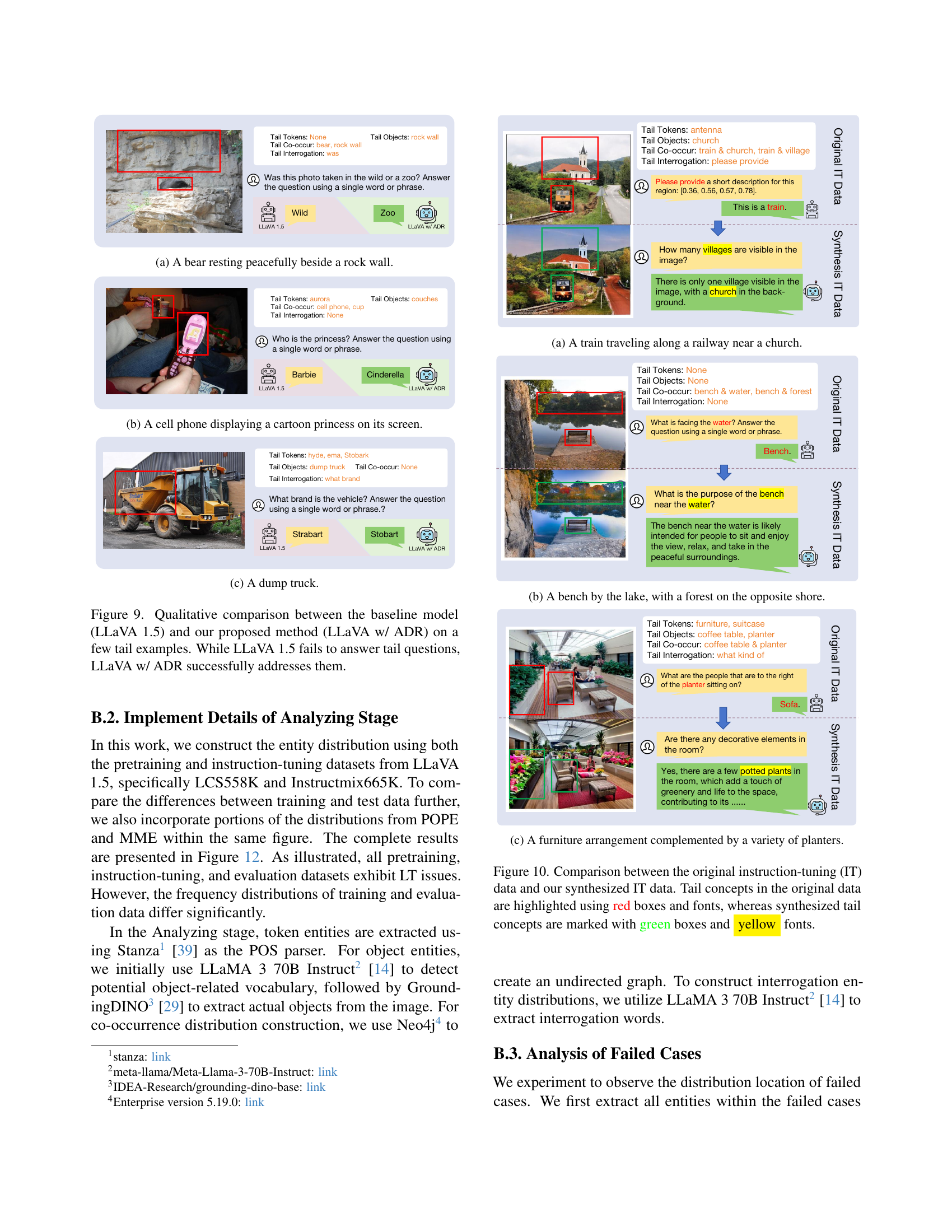
🔼 This figure presents a qualitative comparison of LLaVA 1.5 (baseline) and LLaVA with ADR (the proposed method) on several examples of tail questions (questions related to underrepresented concepts in the training data). The images show that while the baseline model, LLaVA 1.5, fails to answer these challenging, less frequent questions correctly, the model incorporating the ADR framework successfully answers the tail questions. This demonstrates the effectiveness of ADR in improving the model’s ability to handle underrepresented concepts and generalize better to less frequent scenarios.
read the caption
Figure 9: Qualitative comparison between the baseline model (LLaVA 1.5) and our proposed method (LLaVA w/ ADR) on a few tail examples. While LLaVA 1.5 fails to answer tail questions, LLaVA w/ ADR successfully addresses them.

🔼 The image depicts a train traveling on a railway line adjacent to a church. The scene likely represents a rural or suburban area. The railway track is visible, and the train appears to be in motion, possibly suggesting a journey in progress. The church is a prominent feature of the background, and its architectural style and surroundings could offer insights into the local context or history.
read the caption
((a)) A train traveling along a railway near a church.

🔼 The image depicts a wooden bench situated next to a serene lake. Lush greenery, suggestive of a forest, is visible on the opposite bank of the lake. The scene appears tranquil and peaceful, showcasing a natural setting with a simple structure.
read the caption
((b)) A bench by the lake, with a forest on the opposite shore.

🔼 The image shows a living room scene with a variety of furniture pieces, including a coffee table and a sofa. Several potted plants are placed around the room, acting as decorative elements. The overall impression is one of a homey and well-decorated space.
read the caption
((c)) A furniture arrangement complemented by a variety of planters.

🔼 Figure 10 displays a comparison of original and synthesized instruction-tuning data. The figure highlights the differences in the representation of ’tail concepts’ – concepts that are under-represented in the original dataset. The original data’s tail concepts are shown in red boxes and fonts, while those generated through the data synthesis process in the proposed ADR framework are highlighted in green boxes and yellow fonts. This visual comparison demonstrates the effectiveness of the data synthesis stage in enriching the dataset with more examples of under-represented concepts.
read the caption
Figure 10: Comparison between the original instruction-tuning (IT) data and our synthesized IT data. Tail concepts in the original data are highlighted using red boxes and fonts, whereas synthesized tail concepts are marked with green boxes and yellow fonts.

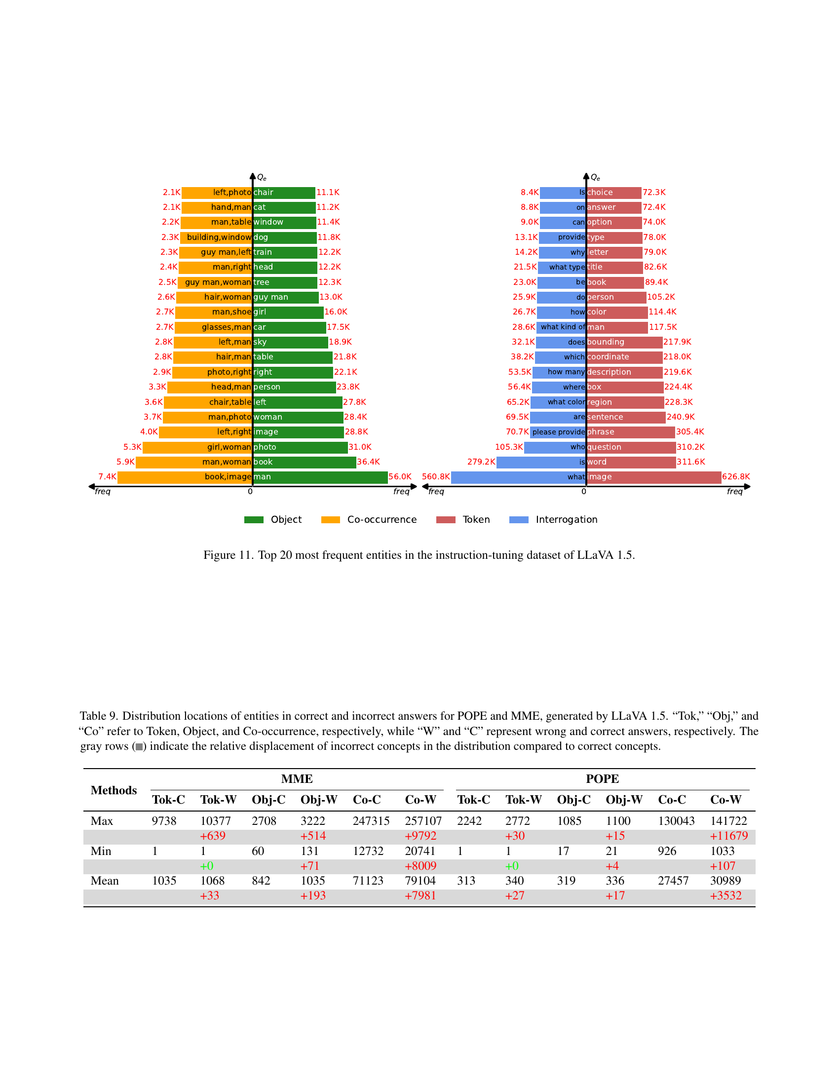
🔼 This bar chart visualizes the top 20 most frequent entities across four categories (tokens, objects, co-occurrences, and interrogations) within the instruction-tuning dataset used to train the LLaVA 1.5 large vision-language model. For each entity, the bar’s height represents its frequency of occurrence in the dataset. The chart offers insights into the prevalent themes and concepts within the training data, highlighting which aspects are most heavily represented and thus may influence the model’s performance and potential biases.
read the caption
Figure 11: Top 20 most frequent entities in the instruction-tuning dataset of LLaVA 1.5.

🔼 This figure shows the token-level word distribution in the MME dataset. The graph displays the frequency distribution of different words, highlighting the long-tail phenomenon where a small number of frequent words make up a large proportion of the data, while a vast number of infrequent words constitute the remaining portion.
read the caption
((a)) MME: Tok

🔼 This figure shows the token-level word distribution in the LCS558K dataset. The x-axis represents the word frequency, and the y-axis represents the relative frequency of words. The graph visualizes the long-tail distribution of words in the dataset, indicating a significant imbalance in the distribution of word frequencies. Many words appear infrequently, while a few words appear very frequently. This is typical of natural language data and highlights the long-tail problem which the paper attempts to address.
read the caption
((b)) LCS558K: Tok

🔼 This figure shows the token-level word distribution in the InstructMix665K dataset. It’s a histogram illustrating the frequency of different words. The x-axis represents the words and the y-axis represents their frequency or relative count in the dataset. This visualization helps to understand the distribution of words, showing which words are frequent and which words are rare.
read the caption
((c)) InstructMix665K: Tok

🔼 This figure shows the object-level word distribution in the MME benchmark dataset. It illustrates the frequency of different object words within the dataset, highlighting the imbalance in representation. The x-axis represents the object words, and the y-axis represents their frequency or proportion in the dataset. The graph visually demonstrates the long-tail distribution characteristic of the MME dataset where some object categories are highly frequent, while others are very infrequent.
read the caption
((d)) MME: Obj

🔼 This figure shows the object-level word distribution in the LCS558K dataset. The x-axis represents the word, and the y-axis represents the frequency. The plot displays the distribution of object words within the training data of the LCS558K dataset. It illustrates the imbalance in the data, showing the presence of a long tail, indicating that many objects have low frequency counts, while a few objects have very high frequency counts. This plot helps to visualize the long-tail problem in the dataset and how this data imbalance may affect the performance of Large Vision-Language Models (LVLMs).
read the caption
((e)) LCS558K: Obj

🔼 This figure shows the object-level word distribution in the InstructMix665K dataset. The x-axis represents the words, and the y-axis represents their relative frequency. The distribution illustrates the long-tail phenomenon, where a small number of objects account for a large proportion of the data, while a vast number of objects are sparsely represented. This visualization highlights the imbalance in the dataset, demonstrating the challenge posed by long-tail data for training effective vision-language models.
read the caption
((f)) InstructMix665K: Obj
More on tables
| Data | Level | thres | % E | % DI |
| MME [16] | Tok | 156 | 99.98 | 75.23 |
| Obj | 153 | 99.83 | 51.33 | |
| Co | 7448 | 99.02 | 69.62 | |
| POPE [25] | Tok | 120 | 99.98 | 80.50 |
| Obj | 90 | 99.71 | 59.76 | |
| Co | 3496 | 99.54 | 75.45 | |
| Avg. | - | - | 99.68 | 68.65 |
🔼 This table presents an analysis of the long-tail problem in Large Vision-Language Models (LVLMs). It focuses on the portion of training data associated with the 50% of cases where the model failed to produce a correct answer. For each of three data categories (tokens, objects, and co-occurrences), the table shows the percentage of tail entities (%E) and the percentage of tail data instances (%DI) contained within the 50% of failed cases. This highlights the disproportionate impact of underrepresented data on model failures.
read the caption
Table 2: Relative training data volume for the tail 50% of failed cases. “Tok”, “Obj”, and “Co” refer to Token, Object, and Co-occurrence, respectively. %E denotes the percentage of tail entities, while %DI represents the percentage of tail data instances.
| Method | IT* | VQA | SEED | QB | MMS | MME | SQA | MMMU | VQA | GQA | MMB | VQA |
|---|---|---|---|---|---|---|---|---|---|---|---|---|
| LLaVA 1.5 | 665.0K | 53.2 | 48.7 | 47.3 | 33.5 | 1510.7 | 69.3 | 35.3 | 46.0 | 61.9 | 64.3 | 76.6 |
| +DR | 581.0K | 55.3 | 57.2 | 46.8 | 33.8 | 1470.6 | 69.5 | 34.8 | 46.0 | 62.8 | 65.5 | 76.9 |
| +DR +DS | 665.0K | 57.4 | 57.4 | 49.6 | 35.5 | 1512.8 | 70.4 | 36.7 | 47.2 | 62.9 | 65.0 | 76.9 |
| ShareGPT4V | 1246.0K | 54.0 | 59.6 | 44.2 | 34.7 | 1560.4 | 68.9 | 35.1 | 50.2 | 63.3 | 68.0 | 78.6 |
| +DR | 1168.0K | 56.7 | 59.6 | 44.9 | 35.0 | 1542.3 | 68.6 | 35.7 | 50.9 | 63.9 | 67.9 | 78.7 |
| +DR +DS | 1246.0K | 57.9 | 59.9 | 45.7 | 35.5 | 1564.9 | 69.4 | 36.1 | 50.9 | 63.7 | 68.8 | 78.7 |
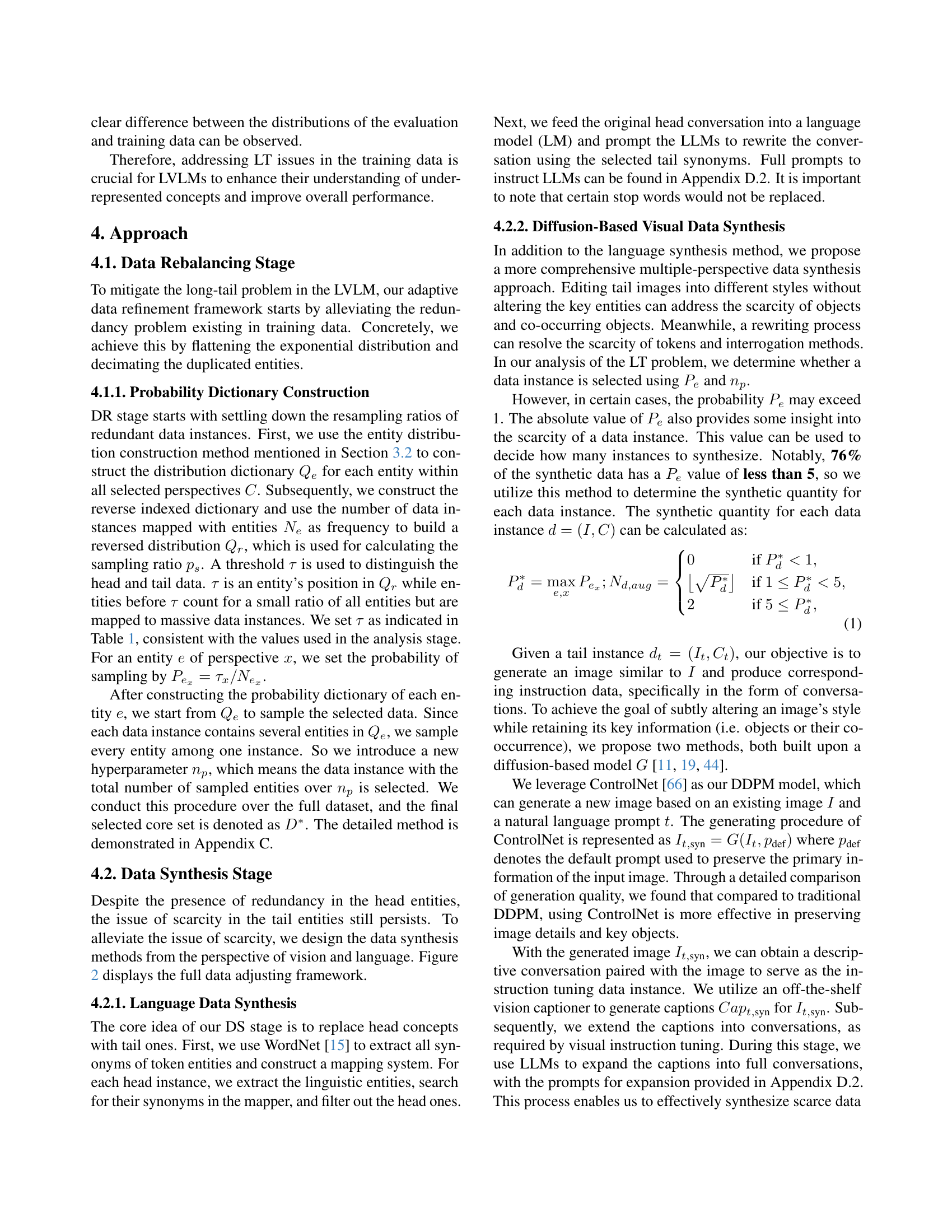
🔼 This table compares the performance of several large vision-language models (LVLMs) on eleven benchmark datasets. The models were trained using different methods: a baseline LLaVA 1.5 model, the same model with data rebalancing (+DR), the rebalanced model with data synthesis (+DR+DS), and the ShareGPT4V model with and without data rebalancing (+DR, +DR+DS). The table shows the number of training instances (IT) used for each model and its performance on each benchmark (VQAOK, SEED2, QB2, etc.). ShareGPT4V’s numbers reflect only the second of its three training stages. The best performance in each benchmark is highlighted in bold.
read the caption
Table 3: Comparison with models trained with different methods on different benchmarks. IT represents the number of training instances used during instruction tuning. +DR denotes the results after the data rebalancing stage, while +DS represents the results following the data synthesis stage. Benchmark names are abbreviated due to space limits. *: ShareGPT4V’s instruction tuning stage refers to the 2nd stage (3 in total). The best results are indicated in bold.
| Method | IT | GQA | SEED | SEED | POPE | MMB |
|---|---|---|---|---|---|---|
| Baseline | 665K | 62.0 | 61.0 | 57.2 | 87.2 | 65.5 |
| EL2N | 581K | 62.5 | 53.6 | 47.4 | 87.2 | 65.2 |
| Perplexity | 581K | 62.3 | 53.4 | 47.4 | 86.8 | 63.7 |
| CLIP Score | 581K | 62.5 | 53.0 | 47.0 | 87.0 | 64.5 |
| COINCIDE | 133K | 59.8 | - | - | 86.1 | 63.1 |
| Ours-DR | 581K | 62.8 | 61.0 | 57.2 | 87.2 | 65.5 |
| Ours | 665K | 62.9 | 61.3 | 57.4 | 87.4 | 65.0 |
🔼 This table compares the performance of different data balancing methods on various benchmarks, specifically focusing on general-purpose visual and language understanding tasks. The methods are evaluated based on their performance on the GQA, SEED, SEEDV2, POPE, and MMB benchmarks. The table highlights the best performing method for each metric in bold and the second-best in underline. The number of training instances (IT) used in instruction tuning for each method is also included, providing context for the performance comparison. The table provides insights into the effectiveness of various data balancing techniques for improving the performance of large vision-language models.
read the caption
Table 4: Performance comparison across existing data balancing methods. The best results are indicated in bold, and the second-best results are underlined. IT represents the number of training instances used during instruction tuning.
| Methods | IT | ScienceQA | |||||
|---|---|---|---|---|---|---|---|
| @5 | @10 | @15 | @20 | H@80 | Overall | ||
| LLaVA 1.5 | 665.0K | 67.9 | 70.0 | 67.9 | 68.5 | 74.6 | 69.3 |
| +DR | 581.0K | 69.2 | 69.7 | 67.8 | 68.5 | 76.2 | 69.5 |
| +DR +DS | 665.0K | 70.1 | 70.5 | 68.3 | 69.0 | 78.6 | 70.2 |
🔼 This table presents a detailed analysis of the model’s performance on the ScienceQA-IMG dataset, focusing specifically on its ability to accurately predict ’tail concepts.’ Tail concepts refer to those that appear infrequently in the dataset. The table shows prediction accuracy at different thresholds (@k, representing the top k% of tail concepts) and for the top 80% of head concepts (H@k). It compares the baseline performance of LLaVA 1.5 to the performance after applying data rebalancing (+DR) and after both data rebalancing and data synthesis (+DR +DS). The number of training instances used is also provided, allowing for a comparison of performance across different training scales. The best result for each metric is highlighted in bold.
read the caption
Table 5: Tail concept prediction accuracy (%) on ScienceQA-IMG [32] dataset. Tail@k%percent𝑘k\%italic_k % (simplified as @k𝑘kitalic_k), head@k%percent𝑘k\%italic_k % (simplified as H@k𝑘kitalic_k), and overall accuracy are reported. +DR denotes the results after data rebalancing, while +DS represents the results following the data synthesis stage. Bold numbers represent the best results across all methods. IT represents the number of training instances used during instruction tuning.
| Method | IT* | VQA | SEED | QB | MMS | MME | SQA | MMMU | VQA | GQA | MMB | VQA |
|---|---|---|---|---|---|---|---|---|---|---|---|---|
| LLaVA 1.5 | 665.0K | 53.2 | 48.7 | 47.3 | 33.5 | 1510.7 | 69.3 | 35.3 | 46.0 | 61.9 | 64.3 | 76.6 |
| +DR | 581.0K | 55.3 | 57.2 | 46.8 | 33.8 | 1470.6 | 69.5 | 34.8 | 46.0 | 62.8 | 65.5 | 76.9 |
| +DR +DS | 665.0K | 57.4 | 57.4 | 49.6 | 35.5 | 1512.8 | 70.4 | 36.7 | 47.2 | 62.9 | 65.0 | 76.9 |
| +DS 25K | 690.0K | 56.2 | 47.5 | 47.9 | 34.5 | 1486.0 | 68.7 | 36.0 | 47.1 | 62.8 | 66.3 | 77.2 |
| +DS 50K | 715.0K | 57.3 | 47.3 | 47.7 | 35.2 | 1472.5 | 69.9 | 36.9 | 47.0 | 62.7 | 66.3 | 77.1 |
| +DS 100K | 765.0K | 54.5 | 47.2 | 46.1 | 34.6 | 1502.7 | 69.7 | 36.8 | 46.1 | 62.5 | 64.5 | 76.6 |
🔼 Table 6 presents a comparison of several large vision-language models’ performance across various benchmarks. The models are trained using different methods: a baseline model (LLaVA 1.5), a model with data rebalancing (+DR), and models with data rebalancing and varying levels of data synthesis (+DS). The table shows the number of training instances used, and the performance results (scores) for each model and benchmark. The benchmarks are abbreviated for brevity. The best performance for each benchmark is highlighted in bold.
read the caption
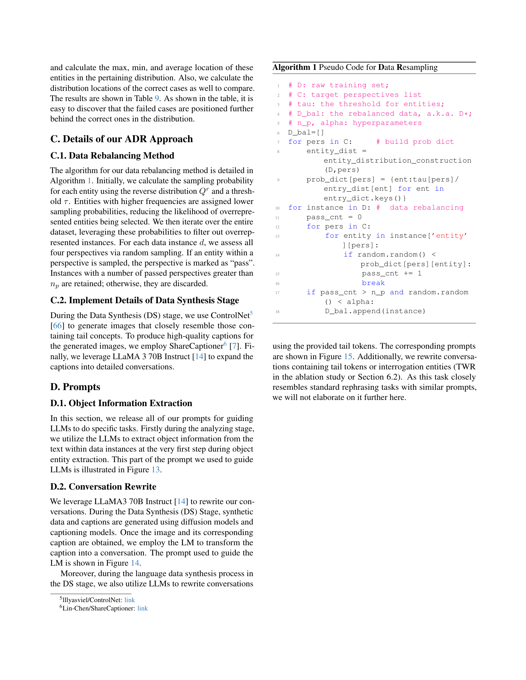
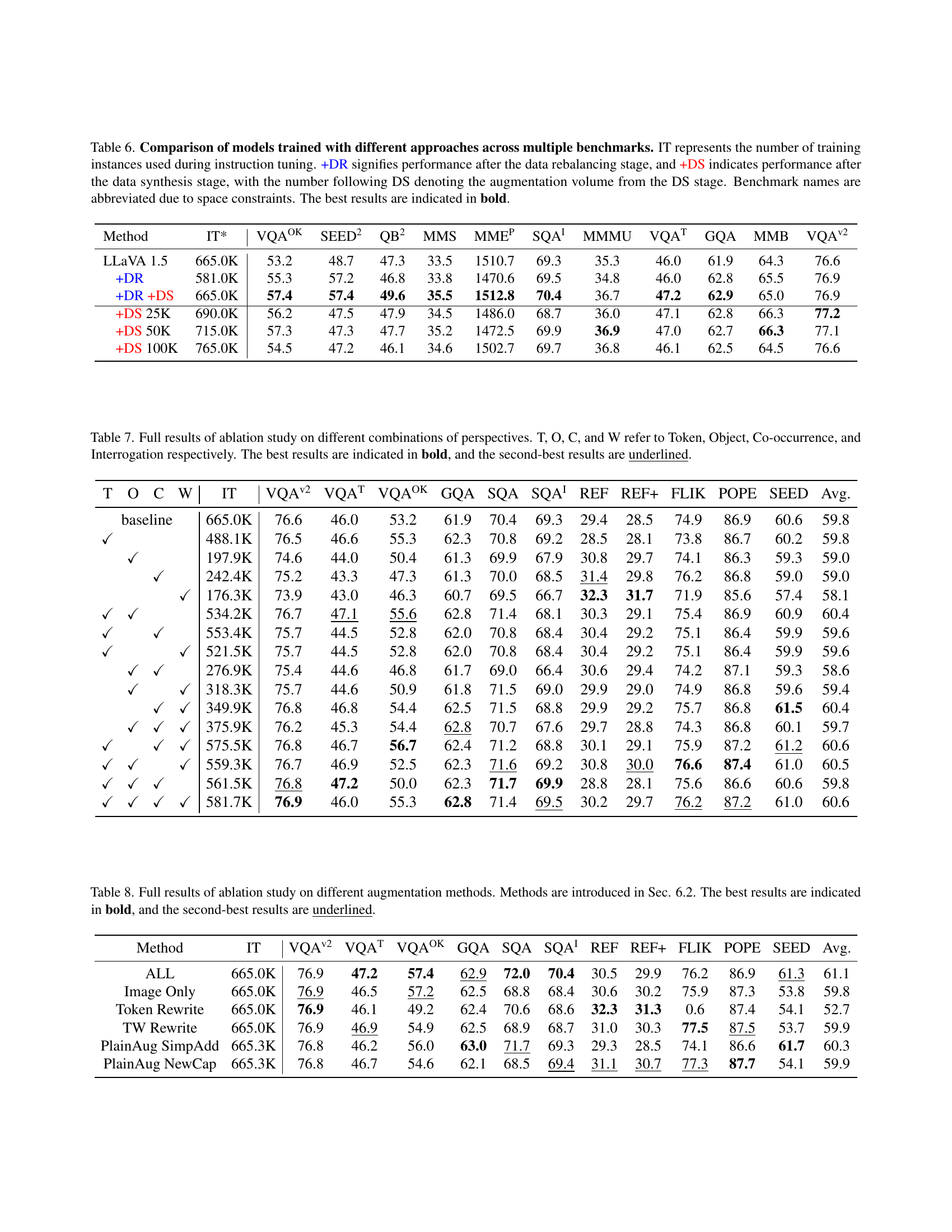
Table 6: Comparison of models trained with different approaches across multiple benchmarks. IT represents the number of training instances used during instruction tuning. +DR signifies performance after the data rebalancing stage, and +DS indicates performance after the data synthesis stage, with the number following DS denoting the augmentation volume from the DS stage. Benchmark names are abbreviated due to space constraints. The best results are indicated in bold.
| T | O | C | W | IT | VQA | VQA | VQA | GQA | SQA | SQA | REF | REF+ | FLIK | POPE | SEED | Avg. |
|---|---|---|---|---|---|---|---|---|---|---|---|---|---|---|---|---|
| baseline | 665.0K | 76.6 | 46.0 | 53.2 | 61.9 | 70.4 | 69.3 | 29.4 | 28.5 | 74.9 | 86.9 | 60.6 | 59.8 | |||
| ✓ | 488.1K | 76.5 | 46.6 | 55.3 | 62.3 | 70.8 | 69.2 | 28.5 | 28.1 | 73.8 | 86.7 | 60.2 | 59.8 | |||
| ✓ | 197.9K | 74.6 | 44.0 | 50.4 | 61.3 | 69.9 | 67.9 | 30.8 | 29.7 | 74.1 | 86.3 | 59.3 | 59.0 | |||
| ✓ | 242.4K | 75.2 | 43.3 | 47.3 | 61.3 | 70.0 | 68.5 | 31.4 | 29.8 | 76.2 | 86.8 | 59.0 | 59.0 | |||
| ✓ | 176.3K | 73.9 | 43.0 | 46.3 | 60.7 | 69.5 | 66.7 | 32.3 | 31.7 | 71.9 | 85.6 | 57.4 | 58.1 | |||
| ✓ | ✓ | 534.2K | 76.7 | 47.1 | 55.6 | 62.8 | 71.4 | 68.1 | 30.3 | 29.1 | 75.4 | 86.9 | 60.9 | 60.4 | ||
| ✓ | ✓ | 553.4K | 75.7 | 44.5 | 52.8 | 62.0 | 70.8 | 68.4 | 30.4 | 29.2 | 75.1 | 86.4 | 59.9 | 59.6 | ||
| ✓ | ✓ | 521.5K | 75.7 | 44.5 | 52.8 | 62.0 | 70.8 | 68.4 | 30.4 | 29.2 | 75.1 | 86.4 | 59.9 | 59.6 | ||
| ✓ | ✓ | 276.9K | 75.4 | 44.6 | 46.8 | 61.7 | 69.0 | 66.4 | 30.6 | 29.4 | 74.2 | 87.1 | 59.3 | 58.6 | ||
| ✓ | ✓ | 318.3K | 75.7 | 44.6 | 50.9 | 61.8 | 71.5 | 69.0 | 29.9 | 29.0 | 74.9 | 86.8 | 59.6 | 59.4 | ||
| ✓ | ✓ | 349.9K | 76.8 | 46.8 | 54.4 | 62.5 | 71.5 | 68.8 | 29.9 | 29.2 | 75.7 | 86.8 | 61.5 | 60.4 | ||
| ✓ | ✓ | ✓ | 375.9K | 76.2 | 45.3 | 54.4 | 62.8 | 70.7 | 67.6 | 29.7 | 28.8 | 74.3 | 86.8 | 60.1 | 59.7 | |
| ✓ | ✓ | ✓ | 575.5K | 76.8 | 46.7 | 56.7 | 62.4 | 71.2 | 68.8 | 30.1 | 29.1 | 75.9 | 87.2 | 61.2 | 60.6 | |
| ✓ | ✓ | ✓ | 559.3K | 76.7 | 46.9 | 52.5 | 62.3 | 71.6 | 69.2 | 30.8 | 30.0 | 76.6 | 87.4 | 61.0 | 60.5 | |
| ✓ | ✓ | ✓ | 561.5K | 76.8 | 47.2 | 50.0 | 62.3 | 71.7 | 69.9 | 28.8 | 28.1 | 75.6 | 86.6 | 60.6 | 59.8 | |
| ✓ | ✓ | ✓ | ✓ | 581.7K | 76.9 | 46.0 | 55.3 | 62.8 | 71.4 | 69.5 | 30.2 | 29.7 | 76.2 | 87.2 | 61.0 | 60.6 |
🔼 Table 7 presents a comprehensive ablation study analyzing the impact of different combinations of perspectives (Token, Object, Co-occurrence, and Interrogation) on the performance of a large vision-language model. The table shows the results across various evaluation metrics on several benchmarks. Each row represents a unique combination of perspectives used for data refinement, enabling the assessment of the individual contribution of each aspect to the overall model performance. The best-performing combination for each metric is highlighted in bold, with the second-best underlined. This allows for a detailed comparison of model performance under various data refinement strategies.
read the caption
Table 7: Full results of ablation study on different combinations of perspectives. T, O, C, and W refer to Token, Object, Co-occurrence, and Interrogation respectively. The best results are indicated in bold, and the second-best results are underlined.
| Method | IT | VQA | VQA | VQA | GQA | SQA | SQA | REF | REF+ | FLIK | POPE | SEED | Avg. |
|---|---|---|---|---|---|---|---|---|---|---|---|---|---|
| ALL | 665.0K | 76.9 | 47.2 | 57.4 | 62.9 | 72.0 | 70.4 | 30.5 | 29.9 | 76.2 | 86.9 | 61.3 | 61.1 |
| Image Only | 665.0K | 76.9 | 46.5 | 57.2 | 62.5 | 68.8 | 68.4 | 30.6 | 30.2 | 75.9 | 87.3 | 53.8 | 59.8 |
| Token Rewrite | 665.0K | 76.9 | 46.1 | 49.2 | 62.4 | 70.6 | 68.6 | 32.3 | 31.3 | 0.6 | 87.4 | 54.1 | 52.7 |
| TW Rewrite | 665.0K | 76.9 | 46.9 | 54.9 | 62.5 | 68.9 | 68.7 | 31.0 | 30.3 | 77.5 | 87.5 | 53.7 | 59.9 |
| PlainAug SimpAdd | 665.3K | 76.8 | 46.2 | 56.0 | 63.0 | 71.7 | 69.3 | 29.3 | 28.5 | 74.1 | 86.6 | 61.7 | 60.3 |
| PlainAug NewCap | 665.3K | 76.8 | 46.7 | 54.6 | 62.1 | 68.5 | 69.4 | 31.1 | 30.7 | 77.3 | 87.7 | 54.1 | 59.9 |
🔼 This table presents a comprehensive ablation study comparing various data augmentation methods used in the Data Synthesis stage of the Adaptive Data Refinement Framework (ADR). The study evaluates six different techniques for generating synthetic data to address the long-tail problem in large vision-language models. Each method is tested on multiple benchmark datasets, and the results (average scores across multiple metrics) are shown. The best and second-best results for each benchmark are highlighted in bold and underlined, respectively. This allows for a detailed comparison of the effectiveness of each augmentation strategy in improving model performance, specifically focusing on tail concepts (under-represented data). The table provides valuable insights into the optimal synthesis method within the ADR framework.
read the caption
Table 8: Full results of ablation study on different augmentation methods. Methods are introduced in Sec. 6.2. The best results are indicated in bold, and the second-best results are underlined.
| Methods | MME | POPE | ||||||||||
|---|---|---|---|---|---|---|---|---|---|---|---|---|
| Tok-C | Tok-W | Obj-C | Obj-W | Co-C | Co-W | Tok-C | Tok-W | Obj-C | Obj-W | Co-C | Co-W | |
| Max | 9738 | 10377 | 2708 | 3222 | 247315 | 257107 | 2242 | 2772 | 1085 | 1100 | 130043 | 141722 |
| +639 | +514 | +9792 | +30 | +15 | +11679 | |||||||
| Min | 1 | 1 | 60 | 131 | 12732 | 20741 | 1 | 1 | 17 | 21 | 926 | 1033 |
| +0 | +71 | +8009 | +0 | +4 | +107 | |||||||
| Mean | 1035 | 1068 | 842 | 1035 | 71123 | 79104 | 313 | 340 | 319 | 336 | 27457 | 30989 |
| +33 | +193 | +7981 | +27 | +17 | +3532 | |||||||
🔼 Table 9 presents a comparative analysis of the distribution of entities (tokens, objects, and co-occurrences) in both correct and incorrect answers generated by the LLaVA 1.5 model on the POPE and MME benchmarks. The table quantifies the maximum, minimum, and average positions of these entities within their respective distributions. The highlighted rows show the difference in the average position between correct and incorrect answers, illustrating the tendency for incorrect responses to involve entities located further towards the tail of the distribution.
read the caption
Table 9: Distribution locations of entities in correct and incorrect answers for POPE and MME, generated by LLaVA 1.5. “Tok,” “Obj,” and “Co” refer to Token, Object, and Co-occurrence, respectively, while “W” and “C” represent wrong and correct answers, respectively. The gray rows ( ) indicate the relative displacement of incorrect concepts in the distribution compared to correct concepts.
Full paper#