TL;DR#
Current LLMs are capable of solving reasoning-intensive tasks, but their inference-time optimization presents challenges. Existing search-based methods often struggle with excessive exploration, while auto-regressive generation lacks global awareness. This results in either inefficient computation or suboptimal performance. There is also room for better resource management so that more computation can be allocated to where it matters most.
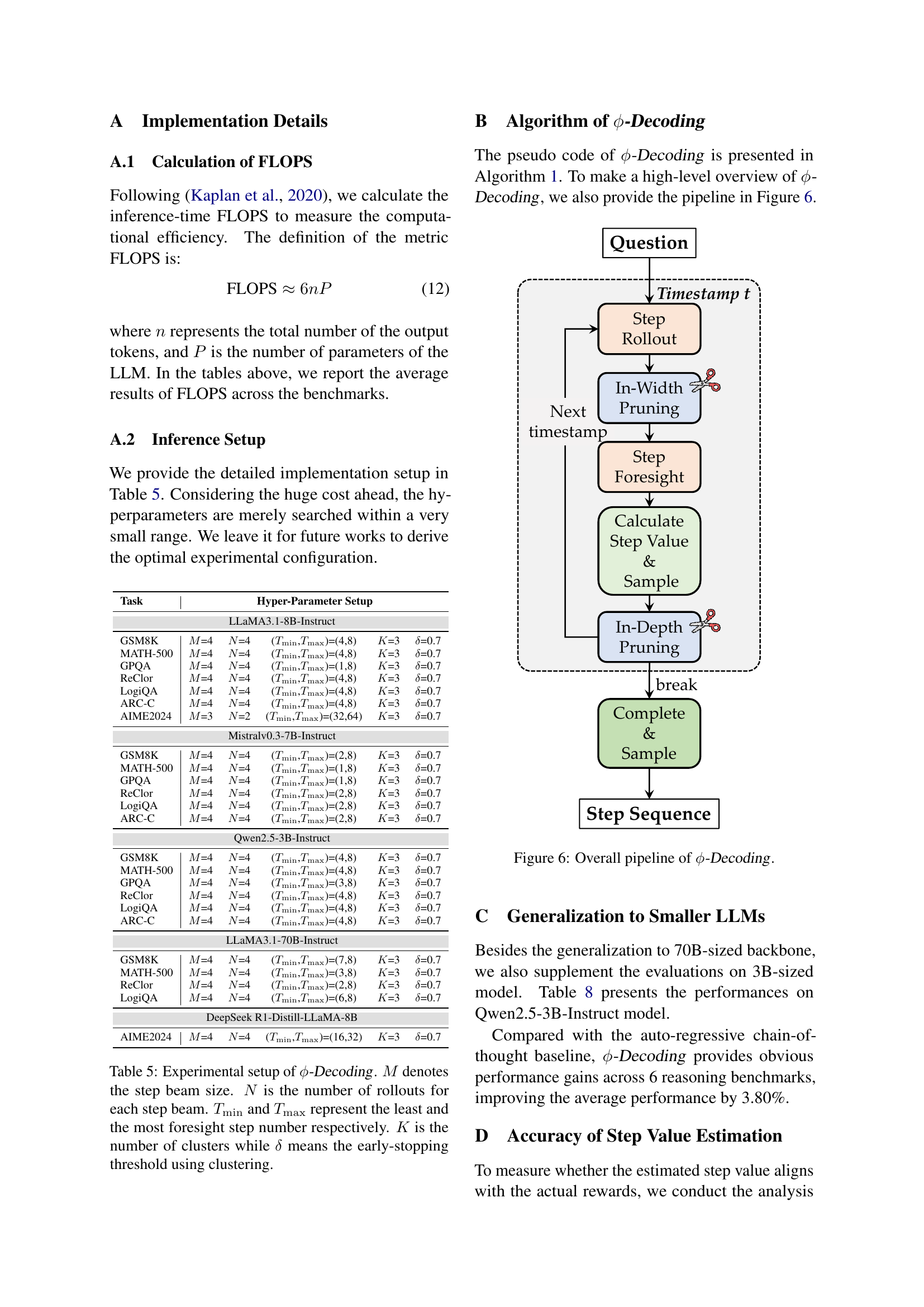
This paper addresses these issues by framing the decoding strategy as foresight sampling and introducing Φ-Decoding. This novel approach leverages simulated future steps to estimate step value and adaptively balances exploration and exploitation. This method is shown to outperform existing approaches in both performance and efficiency across multiple benchmarks, offering superior generalization and scalability.
Key Takeaways#
Why does it matter?#
This paper introduces a novel decoding strategy, providing a more effective way for LLMs to tackle reasoning tasks. Its broad applicability and efficiency gains make it a valuable resource, opening doors for enhanced LLM performance with better resource management.
Visual Insights#

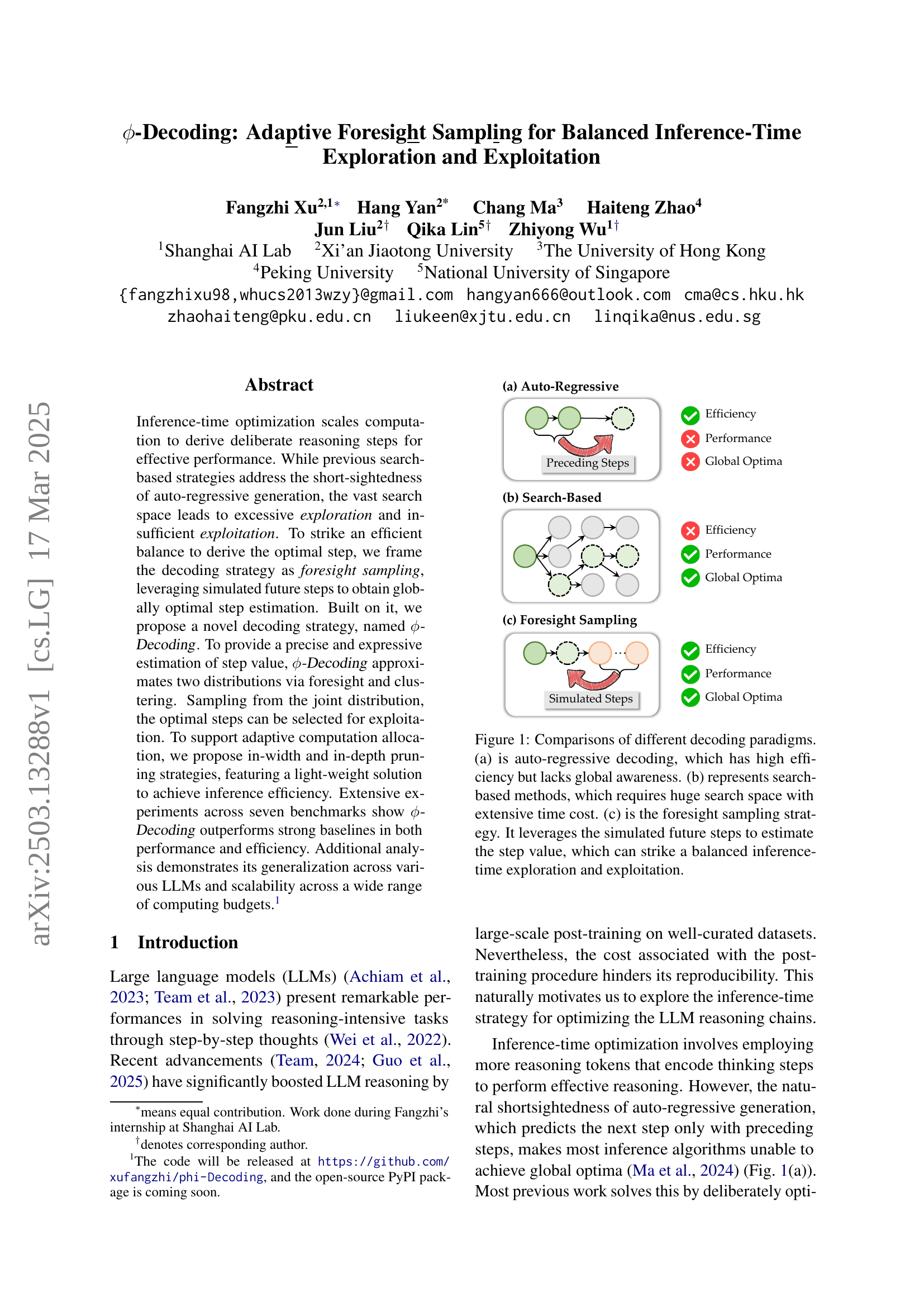
🔼 This figure compares three different decoding paradigms for large language models (LLMs): auto-regressive decoding, search-based methods, and foresight sampling. Auto-regressive decoding is efficient but lacks global awareness, meaning it only considers preceding steps when generating the next one. Search-based methods explore the vast search space of possible steps but are computationally expensive. Foresight sampling strikes a balance by using simulated future steps to estimate the optimal step, improving both efficiency and global awareness.
read the caption
Figure 1: Comparisons of different decoding paradigms. (a) is auto-regressive decoding, which has high efficiency but lacks global awareness. (b) represents search-based methods, which requires huge search space with extensive time cost. (c) is the foresight sampling strategy. It leverages the simulated future steps to estimate the step value, which can strike a balanced inference-time exploration and exploitation.
| Models | GSM8K | Math-500 | GPQA | ReClor | LogiQA | ARC-c | Avg. | FLOPS |
| LLaMA3.1-8B-Instruct | ||||||||
| Auto-Regressive (CoT) | 70.28 | 31.00 | 26.56 | 49.40 | 33.33 | 58.91 | 44.91 | |
| Tree-of-Thoughts | 75.74 | 31.60 | 31.25 | 59.00 | 45.93 | 80.72 | 54.04 | |
| MCTS | 80.44 | 34.40 | 24.11 | 61.40 | 42.70 | 79.95 | 53.83 | |
| Guided Decoding | 75.51 | 31.20 | 30.58 | 60.20 | 43.47 | 81.74 | 53.78 | |
| Predictive Decoding | 81.43 | 34.00 | 31.03 | 64.00 | 46.70 | 84.56 | 56.95 | |
| -Decoding | 86.58 | 38.20 | 34.60 | 64.00 | 48.39 | 85.41 | 59.53 | |
| Mistral-v0.3-7B-Instruct | ||||||||
| Auto-Regressive (CoT) | 49.05 | 12.20 | 23.88 | 52.20 | 37.02 | 69.54 | 40.65 | |
| Tree-of-Thoughts | 53.90 | 10.80 | 26.34 | 55.60 | 41.63 | 73.63 | 43.65 | |
| MCTS | 60.12 | 10.80 | 22.77 | 56.80 | 40.71 | 74.74 | 44.32 | |
| Guided Decoding | 53.90 | 10.80 | 27.46 | 53.20 | 36.71 | 73.55 | 42.60 | |
| Predictive Decoding | 58.00 | 11.00 | 22.10 | 54.20 | 39.78 | 73.55 | 43.11 | |
| -Decoding | 60.42 | 16.40 | 29.24 | 58.20 | 43.01 | 78.16 | 47.57 | |
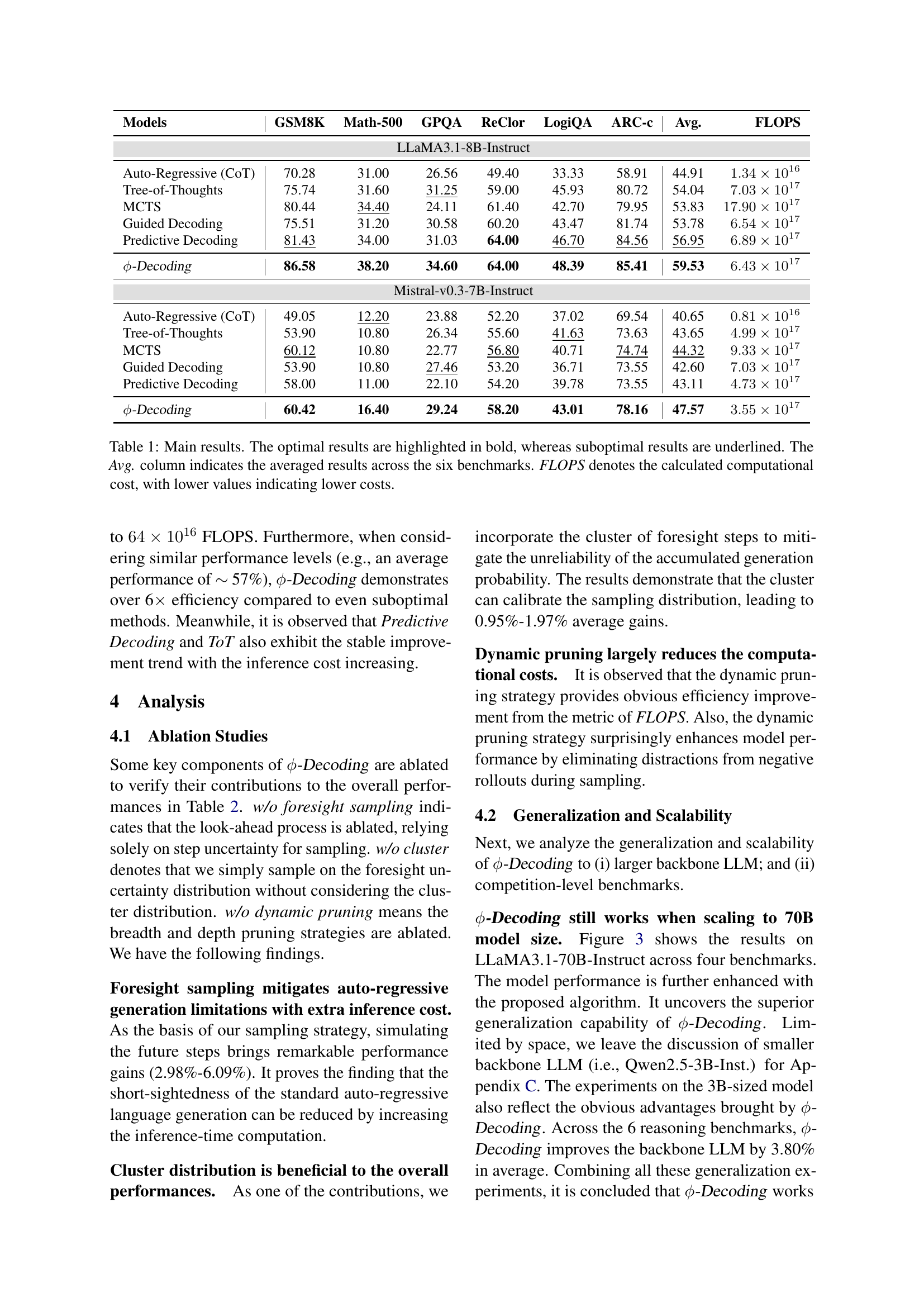
🔼 Table 1 presents the performance comparison of various decoding methods (Auto-Regressive, Tree-of-Thoughts, Monte Carlo Tree Search, Guided Decoding, Predictive Decoding, and Phi-Decoding) across six reasoning benchmarks (GSM8K, MATH-500, GPQA, ReClor, LogiQA, and ARC-Challenge). The table shows the accuracy (Pass@1) achieved by each method on each benchmark, for two different language models (LLaMA3.1-8B-Instruct and Mistral-v0.3-7B-Instruct). The ‘Avg.’ column represents the average accuracy across all six benchmarks for each method. FLOPS (floating point operations per second) indicates the computational cost of each method, providing insights into its efficiency. The optimal results are highlighted in bold, while the suboptimal results are underlined.
read the caption
Table 1: Main results. The optimal results are highlighted in bold, whereas suboptimal results are underlined. The Avg. column indicates the averaged results across the six benchmarks. FLOPS denotes the calculated computational cost, with lower values indicating lower costs.
In-depth insights#
Foresight Decode#
The idea of “Foresight Decode” revolves around improving inference by simulating future steps to better inform current decisions. Unlike autoregressive models that only consider preceding steps, or search-based methods that can be computationally expensive, Foresight Decode strategically samples potential future states. This allows the model to estimate the global optimality of each step, balancing exploration and exploitation. Accurately estimating the step value is critical, often achieved through a process reward model (PRM) or analyzing model uncertainty. The key challenge is balancing computation, focusing resources on difficult steps while conserving compute for simple ones, addressing the issue of ‘overthinking’. Effective implementations involve deriving distributions from foresight paths, combining measures of step advantage and alignment through techniques like clustering. Ultimately, Foresight Decode aims to overcome the limitations of short-sighted generation, leading to more efficient and accurate reasoning.
Adaptive Sampling#
Adaptive sampling in inference-time optimization is crucial for balancing exploration and exploitation. The goal is to intelligently allocate computational resources, focusing on promising reasoning paths while avoiding wasteful exploration of less fruitful avenues. This involves dynamically adjusting the sampling strategy based on the current state of the reasoning process, potentially leveraging foresight to estimate the value of future steps. Effective adaptive sampling requires a mechanism to assess the quality of different steps, guiding the search towards globally optimal solutions while minimizing computational overhead. Techniques like in-width and in-depth pruning, as employed in some methods, exemplify adaptive sampling by strategically reducing the search space, thereby improving both performance and efficiency. The trade-off between accuracy and computational cost is central to adaptive sampling, with the aim of achieving significant performance gains without incurring excessive computational burden. The success of adaptive sampling hinges on the ability to accurately estimate step value, allowing the algorithm to selectively explore and exploit different reasoning paths.
Global Step Value#
Estimating a ‘global step value’ in the context of LLM decoding signifies a crucial aspect of optimizing inference-time strategies. It moves beyond the myopic, auto-regressive approach by considering the broader impact of each step within the reasoning chain. Accurately determining this value allows for a more informed exploration-exploitation balance. A high global step value suggests that the current step is pivotal for achieving the overall task goal, warranting exploitation through focused computation. Conversely, a low value might indicate a need for further exploration of alternative paths. The challenge lies in devising a reliable and efficient method to approximate this global value without incurring excessive computational overhead. Techniques such as foresight sampling (simulating future steps) or leveraging proxy measures like model uncertainty or external reward models could play a key role in determining each step’s worth, leading to substantial performance gains.
Pruning Dynamics#
While ‘Pruning Dynamics’ wasn’t explicitly addressed in this paper, the concept is inherently present in the proposed method’s in-width and in-depth pruning strategies. The paper actively explores and balances the trade-offs between exploration and exploitation, mirroring pruning dynamics. The adaptive nature of $-Decoding allows for a strategic allocation of computational resources, focusing on challenging steps. This dynamic adjustment, eliminating redundant computations and prioritizing critical decision points, directly relates to pruning. By leveraging foresight and cluster-based assessment, $-Decoding dynamically ‘prunes’ less promising paths, leading to efficient and effective reasoning. The observed performance gains, especially with in-depth pruning focusing early, also validates the principle of concentrating on significant components and pruning those that provide marginal utility. This aligns with dynamics where the network adapts, reducing complexity while maintaining robust reasoning.
LLM Scalability#
LLM scalability is a critical area, encompassing model size, dataset volume, and computational resources. Scaling model size, by increasing the number of parameters, often leads to improved performance, but introduces challenges in memory requirements and training time. Techniques like model parallelism and gradient accumulation are vital to enable scaling. Dataset volume plays a crucial role; larger datasets generally result in better generalization and reduced overfitting. However, data quality and diversity are equally important as quantity. Computational resources, particularly GPUs or TPUs, are essential for training and inference. The efficiency of utilizing these resources, through techniques like quantization and knowledge distillation, becomes paramount as models grow. There is need for optimization to achieve significant results, with better computation cost.
More visual insights#
More on figures

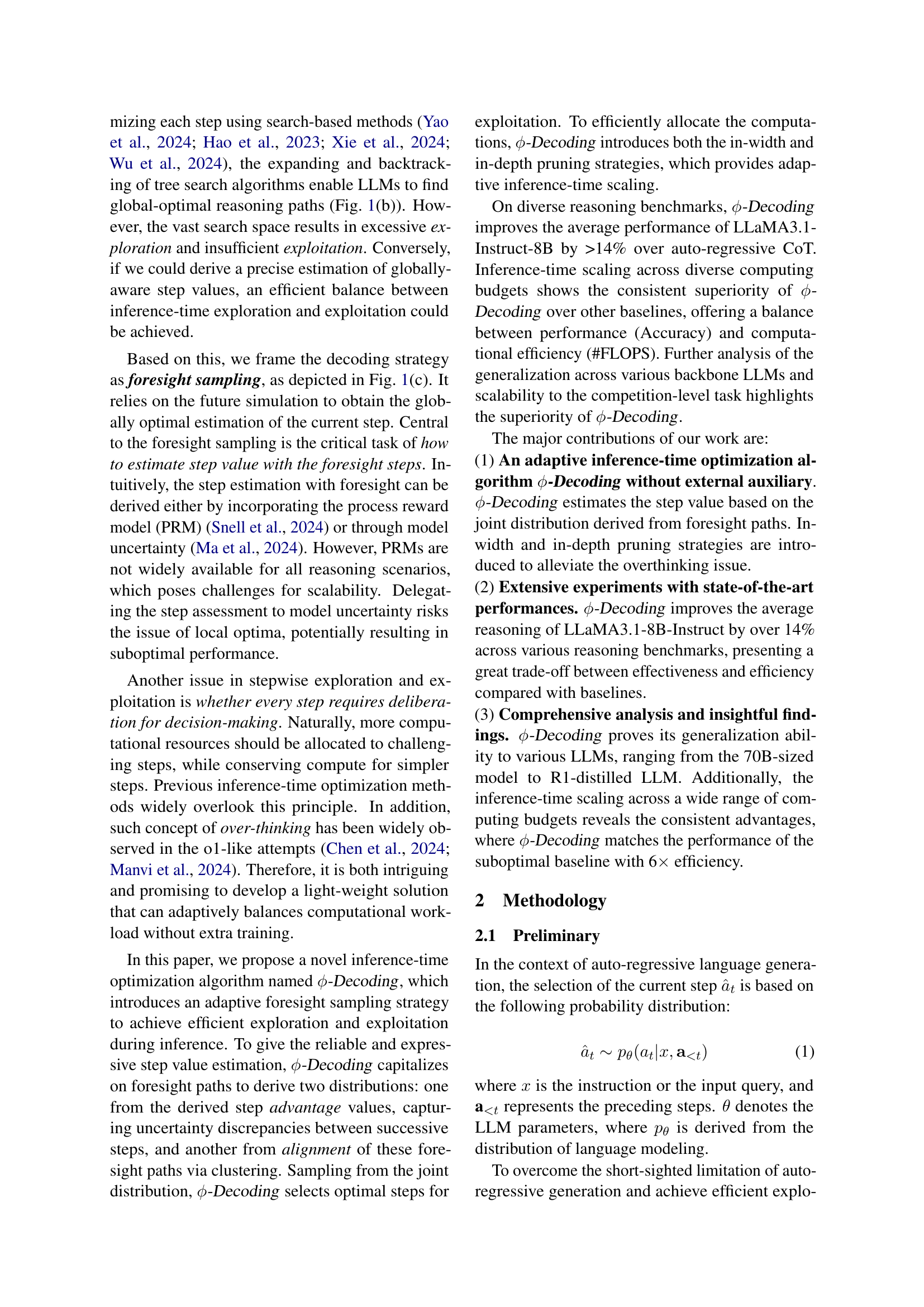
🔼 Figure 2 illustrates the ϕ-Decoding framework, focusing on the decoding process at a single timestamp (t). It simplifies the visualization by using a step beam size (M) of 2, 3 rollouts (N), and 2 clusters (K). The figure shows how ϕ-Decoding uses foresight sampling, in-width pruning, in-depth pruning and cluster alignment to estimate and select optimal steps during inference. It details the steps involved in: step rollout, foresight calculation, advantage and alignment estimation, and final step sampling. The process combines absolute and relative step value estimations to select the best steps for continuation.
read the caption
Figure 2: The overall framework of ϕitalic-ϕ\phiitalic_ϕ-Decoding. We visualize the decoding process at the timestamp t𝑡titalic_t. For simplicity, we set step beam size M𝑀Mitalic_M as 2, the number of rollouts N𝑁Nitalic_N as 3, and the number of clusters K𝐾Kitalic_K as 2.

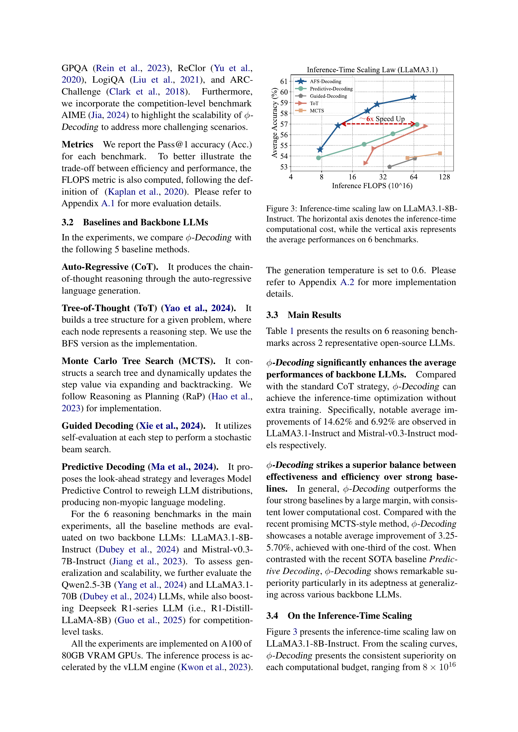
🔼 This figure demonstrates the relationship between inference-time computational cost and model performance across six reasoning benchmarks using the LLaMA3.1-8B-Instruct large language model. The x-axis represents the computational cost (in FLOPS), while the y-axis shows the average performance across the six benchmarks. The graph illustrates how different decoding methods scale with increasing computational resources, showing their trade-off between efficiency and accuracy.
read the caption
Figure 3: Inference-time scaling law on LLaMA3.1-8B-Instruct. The horizontal axis denotes the inference-time computational cost, while the vertical axis represents the average performances on 6 benchmarks.

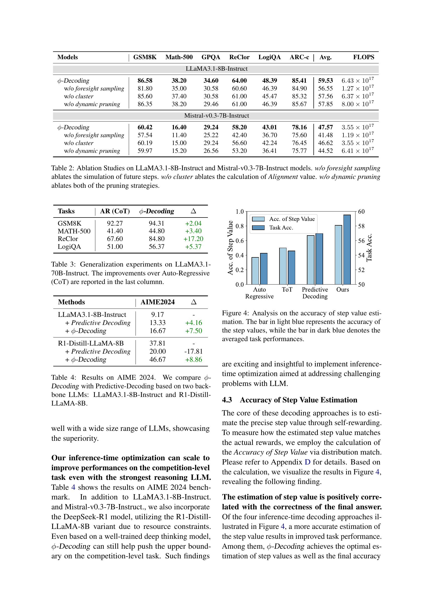
🔼 Figure 4 illustrates the correlation between the accuracy of step value estimation and the overall task performance for four different decoding methods: Autoregressive, Tree-of-Thought, Predictive Decoding, and the proposed φ-Decoding. The light blue bars represent the accuracy of the step value estimations, indicating how well the estimated values reflect the true rewards associated with each step. The dark blue bars show the average task performance achieved by each method. The figure demonstrates that more accurate step value estimation generally leads to better overall task performance, highlighting the importance of precise step value estimation in effective decoding strategies.
read the caption
Figure 4: Analysis on the accuracy of step value estimation. The bar in light blue represents the accuracy of the step values, while the bar in dark blue denotes the averaged task performances.

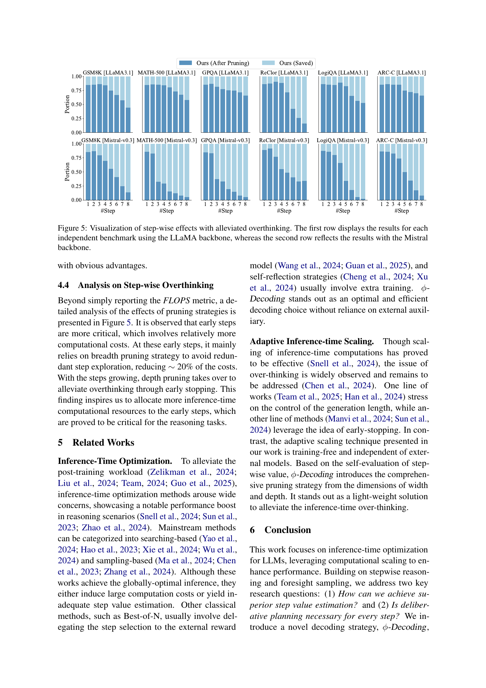
🔼 This figure visualizes how the proposed dynamic pruning strategy in $\$ -Decoding$ effectively manages computational resources across different reasoning steps. The x-axis represents the step number in the reasoning process, and the y-axis indicates the proportion of computational cost (or the number of steps) allocated to each step. The first row shows the results when using LLaMA as the base language model, while the second row presents the findings when using Mistral. The bars in different colors correspond to different benchmarks. We can observe that the pruning strategy allocates more resources to the initial steps of the reasoning process, which are more critical for reaching the correct solution, and gradually reduces resources as the reasoning process progresses. This effectively prevents overthinking by avoiding unnecessary computation in later, less critical steps.
read the caption
Figure 5: Visualization of step-wise effects with alleviated overthinking. The first row displays the results for each independent benchmark using the LLaMA backbone, whereas the second row reflects the results with the Mistral backbone.
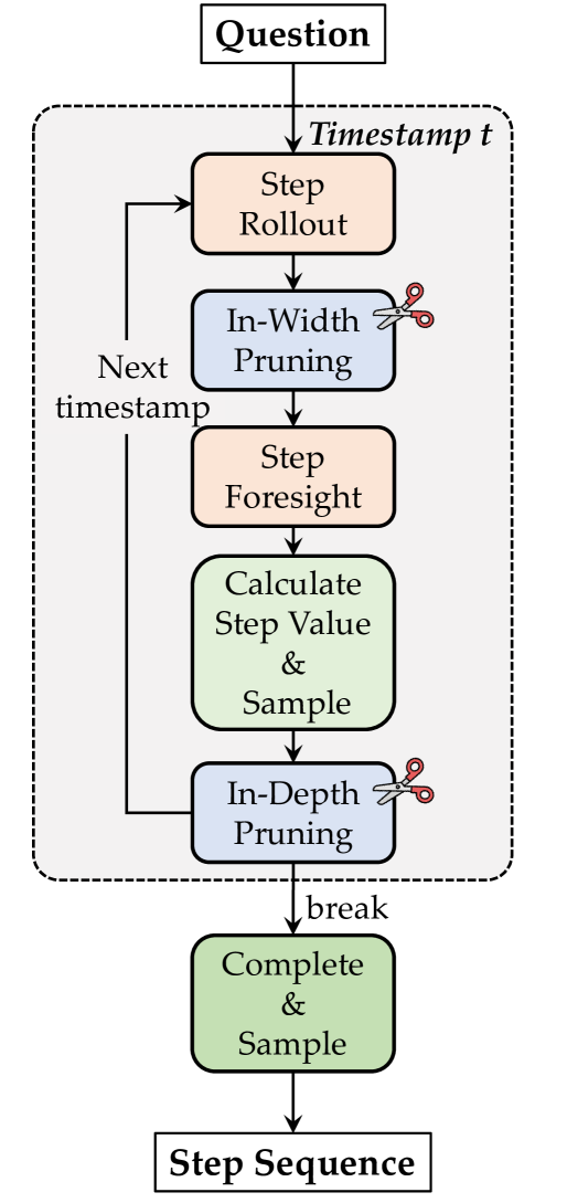
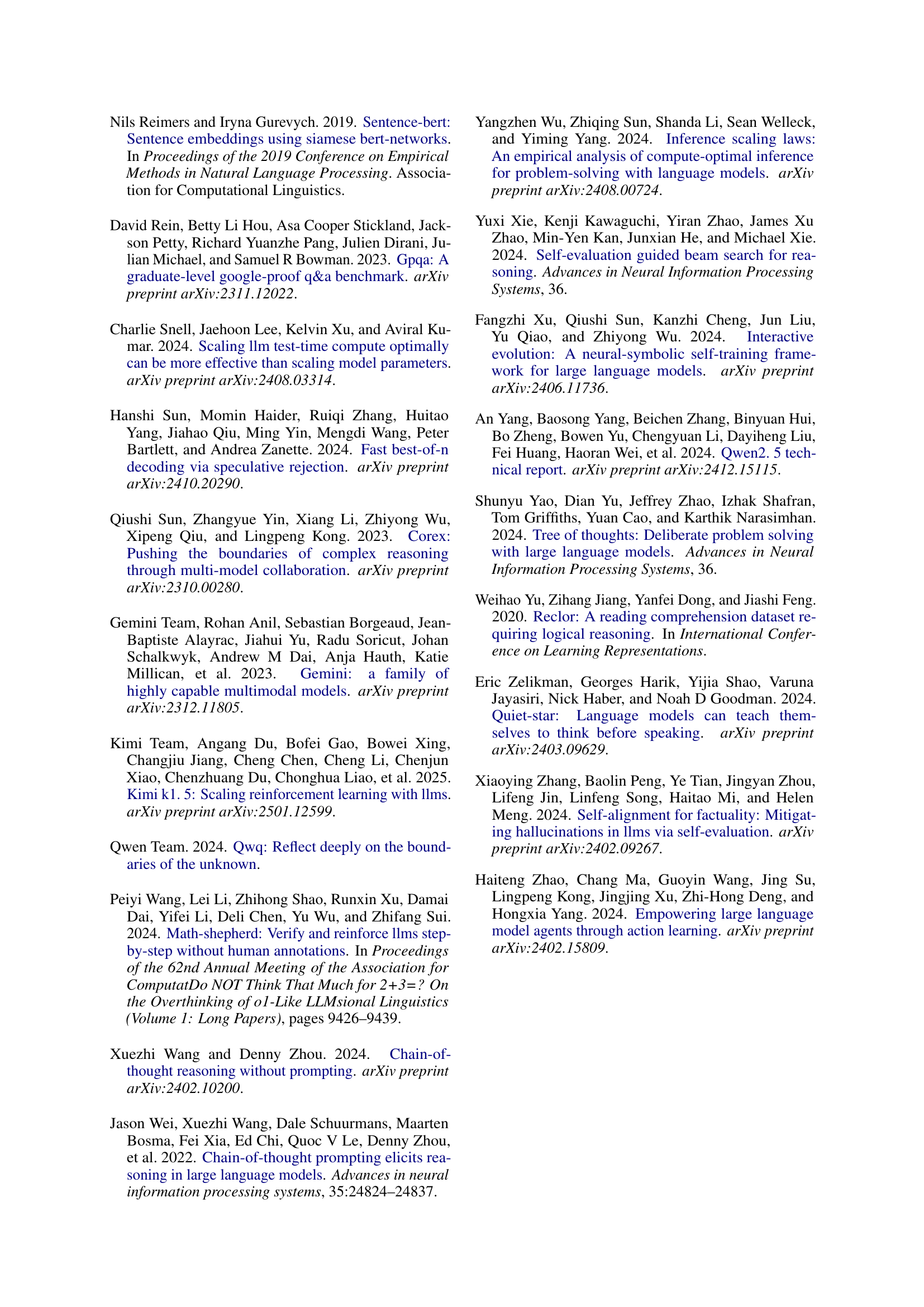
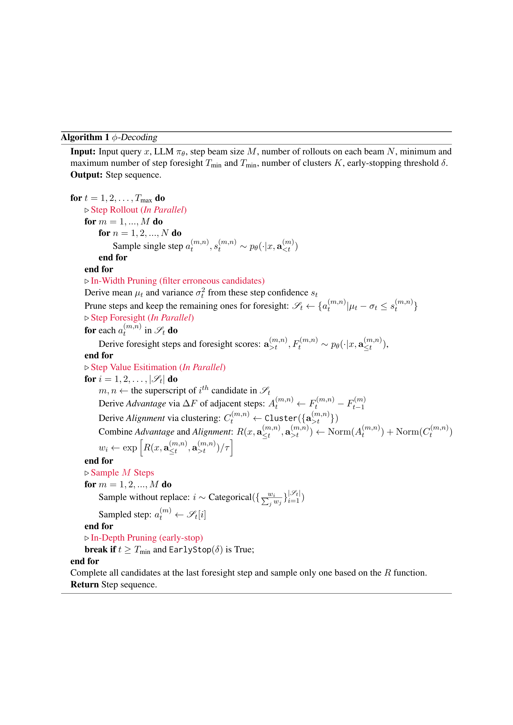
🔼 The figure illustrates the overall pipeline of the ϕ-Decoding algorithm. It starts with an input question, then proceeds through the steps of: step rollout (generating candidate next steps), in-width pruning (filtering less promising candidates), step foresight (simulating the outcomes of choosing each candidate step), step value estimation (calculating how good each candidate step is using foresight information), sampling (selecting the best step based on the estimations), and finally, in-depth pruning (potentially stopping early if the reasoning process is sufficiently advanced). The output is a complete step sequence.
read the caption
Figure 6: Overall pipeline of ϕitalic-ϕ\phiitalic_ϕ-Decoding.
More on tables
| Models | GSM8K | Math-500 | GPQA | ReClor | LogiQA | ARC-c | Avg. | FLOPS |
| LLaMA3.1-8B-Instruct | ||||||||
| -Decoding | 86.58 | 38.20 | 34.60 | 64.00 | 48.39 | 85.41 | 59.53 | |
| w/o foresight sampling | 81.80 | 35.00 | 30.58 | 60.60 | 46.39 | 84.90 | 56.55 | |
| w/o cluster | 85.60 | 37.40 | 30.58 | 61.00 | 45.47 | 85.32 | 57.56 | |
| w/o dynamic pruning | 86.35 | 38.20 | 29.46 | 61.00 | 46.39 | 85.67 | 57.85 | |
| Mistral-v0.3-7B-Instruct | ||||||||
| -Decoding | 60.42 | 16.40 | 29.24 | 58.20 | 43.01 | 78.16 | 47.57 | |
| w/o foresight sampling | 57.54 | 11.40 | 25.22 | 42.40 | 36.70 | 75.60 | 41.48 | |
| w/o cluster | 60.19 | 15.00 | 29.24 | 56.60 | 42.24 | 76.45 | 46.62 | |
| w/o dynamic pruning | 59.97 | 15.20 | 26.56 | 53.20 | 36.41 | 75.77 | 44.52 | |
🔼 This table presents the results of ablation studies conducted on two large language models (LLMs): LLaMA3.1-8B-Instruct and Mistral-v0.3-7B-Instruct. The purpose is to analyze the impact of different components of the proposed -Decoding method on the overall performance. Three variants of the -Decoding method were evaluated: one without foresight sampling, one without cluster analysis for alignment assessment, and one without dynamic pruning. The table shows the average performance (accuracy) across six benchmark tasks for each variant, along with the FLOPS (floating point operations per second) required. This allows for a comparison of performance and efficiency trade-offs for each component of the model.
read the caption
Table 2: Ablation Studies on LLaMA3.1-8B-Instruct and Mistral-v0.3-7B-Instruct models. w/o foresight sampling ablates the simulation of future steps. w/o cluster ablates the calculation of Alignment value. w/o dynamic pruning ablates both of the pruning strategies.
| Tasks | AR (CoT) | -Decoding | |
| GSM8K | 92.27 | 94.31 | +2.04 |
| MATH-500 | 41.40 | 44.80 | +3.40 |
| ReClor | 67.60 | 84.80 | +17.20 |
| LogiQA | 51.00 | 56.37 | +5.37 |
🔼 This table presents the results of generalization experiments conducted using the LLaMA 3.1-70B-Instruct model. It compares the performance of the proposed -Decoding method against the Auto-Regressive Chain of Thought (CoT) baseline across several reasoning tasks (GSM8K, MATH-500, ReClor, and LogiQA). The ‘Acc.’ column shows the accuracy achieved on each task, and the final column highlights the percentage improvement gained by -Decoding over the CoT baseline.
read the caption
Table 3: Generalization experiments on LLaMA3.1-70B-Instruct. The improvements over Auto-Regressive (CoT) are reported in the last columnn.
| Methods | AIME2024 | |
| LLaMA3.1-8B-Instruct | 9.17 | - |
| + Predictive Decoding | 13.33 | +4.16 |
| + -Decoding | 16.67 | +7.50 |
| R1-Distill-LLaMA-8B | 37.81 | - |
| + Predictive Decoding | 20.00 | -17.81 |
| + -Decoding | 46.67 | +8.86 |
🔼 This table presents the performance comparison of ϕ-Decoding and Predictive Decoding on the AIME 2024 benchmark, using two different Large Language Models (LLMs) as backbones: LLaMA3.1-8B-Instruct and R1-Distill-LLaMA-8B. It shows the accuracy achieved by each method on the AIME 2024 dataset, highlighting the improvement that ϕ-Decoding provides over the baseline Predictive-Decoding method across both LLMs.
read the caption
Table 4: Results on AIME 2024. We compare ϕitalic-ϕ\phiitalic_ϕ-Decoding with Predictive-Decoding based on two backbone LLMs: LLaMA3.1-8B-Instruct and R1-Distill-LLaMA-8B.
| Task | Hyper-Parameter Setup | ||||
| LLaMA3.1-8B-Instruct | |||||
| GSM8K | =4 | =4 | (,)=(4,8) | =3 | =0.7 |
| MATH-500 | =4 | =4 | (,)=(4,8) | =3 | =0.7 |
| GPQA | =4 | =4 | (,)=(1,8) | =3 | =0.7 |
| ReClor | =4 | =4 | (,)=(4,8) | =3 | =0.7 |
| LogiQA | =4 | =4 | (,)=(4,8) | =3 | =0.7 |
| ARC-C | =4 | =4 | (,)=(4,8) | =3 | =0.7 |
| AIME2024 | =3 | =2 | (,)=(32,64) | =3 | =0.7 |
| Mistralv0.3-7B-Instruct | |||||
| GSM8K | =4 | =4 | (,)=(2,8) | =3 | =0.7 |
| MATH-500 | =4 | =4 | (,)=(1,8) | =3 | =0.7 |
| GPQA | =4 | =4 | (,)=(1,8) | =3 | =0.7 |
| ReClor | =4 | =4 | (,)=(2,8) | =3 | =0.7 |
| LogiQA | =4 | =4 | (,)=(2,8) | =3 | =0.7 |
| ARC-C | =4 | =4 | (,)=(2,8) | =3 | =0.7 |
| Qwen2.5-3B-Instruct | |||||
| GSM8K | =4 | =4 | (,)=(4,8) | =3 | =0.7 |
| MATH-500 | =4 | =4 | (,)=(4,8) | =3 | =0.7 |
| GPQA | =4 | =4 | (,)=(3,8) | =3 | =0.7 |
| ReClor | =4 | =4 | (,)=(4,8) | =3 | =0.7 |
| LogiQA | =4 | =4 | (,)=(4,8) | =3 | =0.7 |
| ARC-C | =4 | =4 | (,)=(4,8) | =3 | =0.7 |
| LLaMA3.1-70B-Instruct | |||||
| GSM8K | =4 | =4 | (,)=(7,8) | =3 | =0.7 |
| MATH-500 | =4 | =4 | (,)=(3,8) | =3 | =0.7 |
| ReClor | =4 | =4 | (,)=(2,8) | =3 | =0.7 |
| LogiQA | =4 | =4 | (,)=(6,8) | =3 | =0.7 |
| DeepSeek R1-Distill-LLaMA-8B | |||||
| AIME2024 | =4 | =4 | (,)=(16,32) | =3 | =0.7 |
🔼 Table 5 details the settings used in the ϕ-Decoding algorithm. It shows the values for several key hyperparameters that control different aspects of the algorithm’s behavior. These hyperparameters impact the balance between exploration and exploitation during the inference process and the efficiency of computation. Specifically, it defines the size of the beam search (M), the number of future steps simulated (N), the range of foresight steps considered (Tmin and Tmax), the number of clusters used in the clustering step (K), and the threshold for early stopping based on cluster size (δ). Different values for these parameters were used for different tasks and language models to optimize performance.
read the caption
Table 5: Experimental setup of ϕitalic-ϕ\phiitalic_ϕ-Decoding. M𝑀Mitalic_M denotes the step beam size. N𝑁Nitalic_N is the number of rollouts for each step beam. Tminsubscript𝑇minT_{\mathrm{min}}italic_T start_POSTSUBSCRIPT roman_min end_POSTSUBSCRIPT and Tmaxsubscript𝑇maxT_{\mathrm{max}}italic_T start_POSTSUBSCRIPT roman_max end_POSTSUBSCRIPT represent the least and the most foresight step number respectively. K𝐾Kitalic_K is the number of clusters while δ𝛿\deltaitalic_δ means the early-stopping threshold using clustering.
| Cluster Methods | GSM8K | Math-500 | GPQA | ReClor | LogiQA | ARC-c | Avg. | FLOPS |
| -Decoding (LLaMA3.1-8B-Instruct) | ||||||||
| TF-IDF | 86.58 | 38.20 | 34.60 | 64.00 | 48.39 | 85.41 | 59.53 | |
| SBERT (109M) | 86.43 | 39.20 | 33.26 | 63.20 | 47.48 | 85.41 | 59.16 | |
| SBERT (22.7M) | 86.05 | 36.80 | 33.26 | 62.40 | 45.47 | 85.41 | 58.23 | |
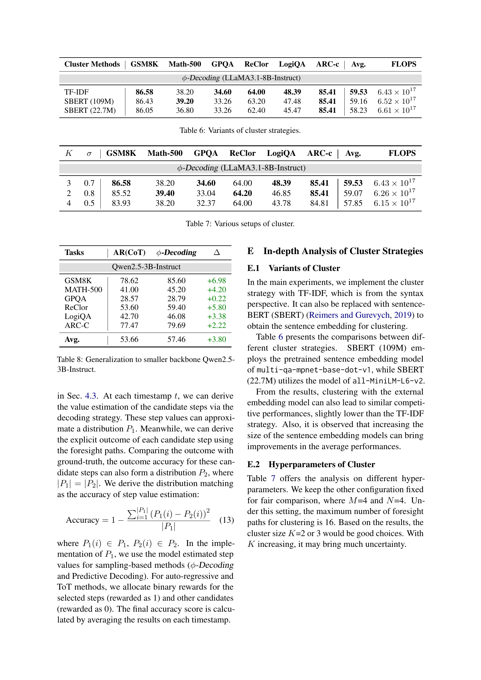
🔼 This table compares different clustering strategies used in the $-Decoding algorithm for step value estimation. It shows the average performance across six reasoning benchmarks (GSM8K, Math-500, GPQA, ReClor, LogiQA, and ARC-Challenge) when using three different clustering methods: TF-IDF, SBERT (109M), and SBERT (22.7M). The results demonstrate the impact of the chosen clustering method on the overall accuracy of the model.
read the caption
Table 6: Variants of cluster strategies.
| GSM8K | Math-500 | GPQA | ReClor | LogiQA | ARC-c | Avg. | FLOPS | ||
| -Decoding (LLaMA3.1-8B-Instruct) | |||||||||
| 3 | 0.7 | 86.58 | 38.20 | 34.60 | 64.00 | 48.39 | 85.41 | 59.53 | |
| 2 | 0.8 | 85.52 | 39.40 | 33.04 | 64.20 | 46.85 | 85.41 | 59.07 | |
| 4 | 0.5 | 83.93 | 38.20 | 32.37 | 64.00 | 43.78 | 84.81 | 57.85 | |
🔼 This table shows the impact of different hyperparameter settings on the performance of the proposed φ-Decoding model. Specifically, it examines how varying the number of clusters (K) used in the clustering-based alignment assessment and the early stopping threshold (δ) affect the overall accuracy and computational cost (FLOPS) across multiple reasoning benchmarks. Different values for K and δ represent different strategies for balancing exploration and exploitation in the search for optimal reasoning steps.
read the caption
Table 7: Various setups of cluster.
| Tasks | AR(CoT) | -Decoding | |
| Qwen2.5-3B-Instruct | |||
| GSM8K | 78.62 | 85.60 | +6.98 |
| MATH-500 | 41.00 | 45.20 | +4.20 |
| GPQA | 28.57 | 28.79 | +0.22 |
| ReClor | 53.60 | 59.40 | +5.80 |
| LogiQA | 42.70 | 46.08 | +3.38 |
| ARC-C | 77.47 | 79.69 | +2.22 |
| Avg. | 53.66 | 57.46 | +3.80 |
🔼 This table presents the results of the generalization experiment performed using a smaller language model, specifically the Qwen2.5-3B-Instruct model. It compares the performance of the proposed method, -Decoding, against the baseline Autoregressive (CoT) method across six reasoning benchmarks. The table displays the accuracy of each method on each benchmark, along with the improvement achieved by -Decoding over the baseline.
read the caption
Table 8: Generalization to smaller backbone Qwen2.5-3B-Instruct.
Full paper#