TL;DR#
Residual connections are crucial in deep learning, but can cause issues like gradient vanishing and representation collapse. Hyper-Connections were introduced to address these problems by using multiple connection strengths. However, Hyper-Connections increase memory access costs. To solve the trade-off between memory usage and expressiveness of connections, this paper introduces Frac-Connections.
Frac-Connections divide hidden states into multiple parts instead of expanding their width. This method retains partial benefits of Hyper-Connections but reduces memory consumption. Experiments on large language tasks, including a 7B MoE model trained on 3T tokens, demonstrate that Frac-Connections significantly outperform residual connections. Frac-Connections shows better training stability and downstream task performance across various NLP benchmarks.
Key Takeaways#
Why does it matter?#
This paper introduces Frac-Connections, an efficient alternative to Hyper-Connections, potentially impacting deep learning architecture design. It offers a novel approach to balancing model performance and memory usage, and opens new avenues for research in optimizing deep learning models.
Visual Insights#

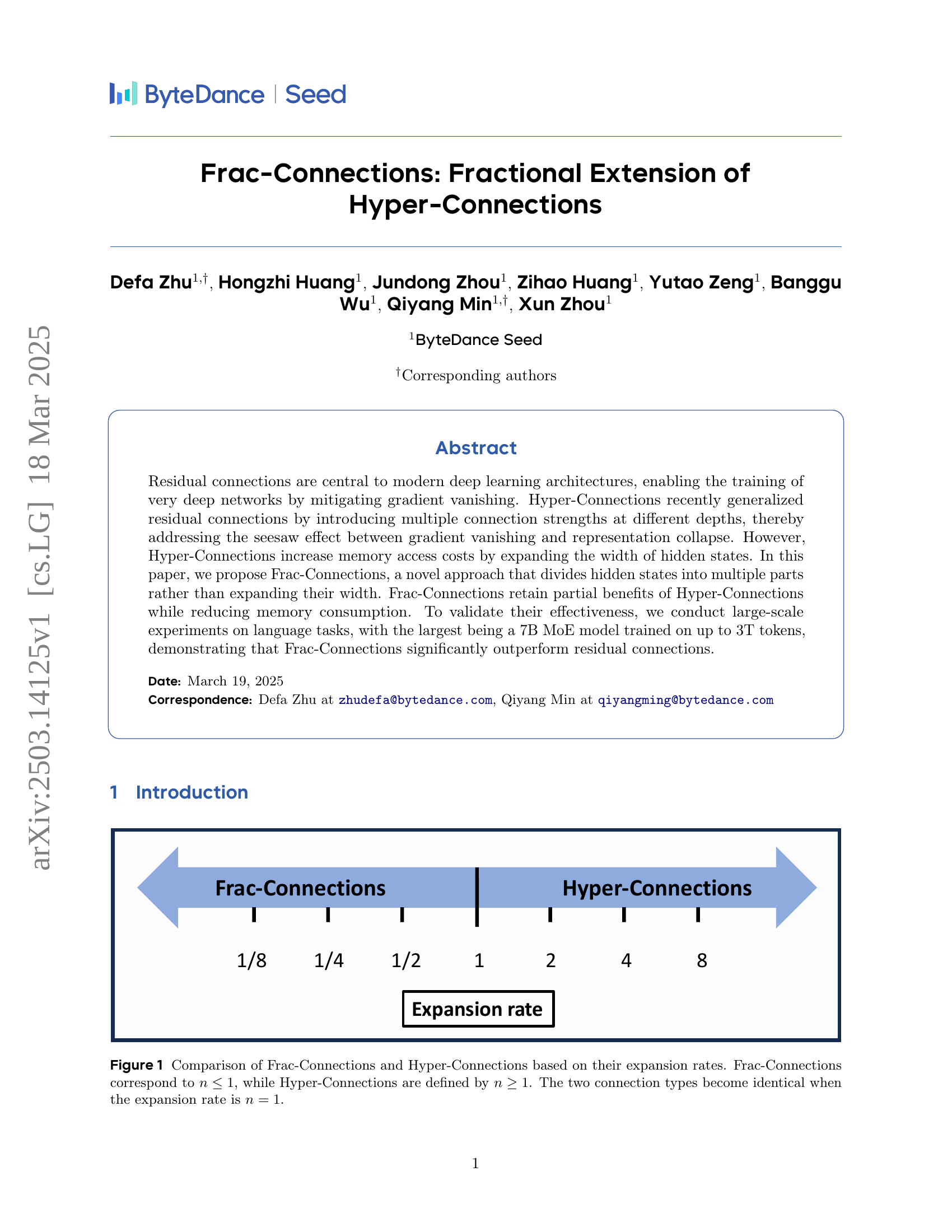
🔼 This figure compares Frac-Connections and Hyper-Connections, two types of residual connections used in deep learning models. The key difference lies in their expansion rate (n). Frac-Connections have an expansion rate of n ≤ 1, meaning they divide the hidden state into multiple parts (the number of parts increases as n decreases towards 0). Hyper-Connections, on the other hand, have an expansion rate of n ≥ 1, where they replicate the hidden state multiple times (the number of replications is n). When n = 1, both connection types are identical. The figure visually represents the relationship between the expansion rate and the type of connection.
read the caption
Figure 1: Comparison of Frac-Connections and Hyper-Connections based on their expansion rates. Frac-Connections correspond to n≤1𝑛1n\leq 1italic_n ≤ 1, while Hyper-Connections are defined by n≥1𝑛1n\geq 1italic_n ≥ 1. The two connection types become identical when the expansion rate is n=1𝑛1n=1italic_n = 1.
| Method | FC Params(B) | Total Params(B) | Total Params rate (%) |
| OLMo-1B2 | - | 1.17676442 | - |
| OLMo-1B2-DFC4 | 0.000165 | 1.17715846 | +0.014% |
| OLMoE-1B-7B | - | 6.91909427 | - |
| OLMoE-1B-7B-DFC4 | 0.000165 | 6.91948832 | +0.0024% |
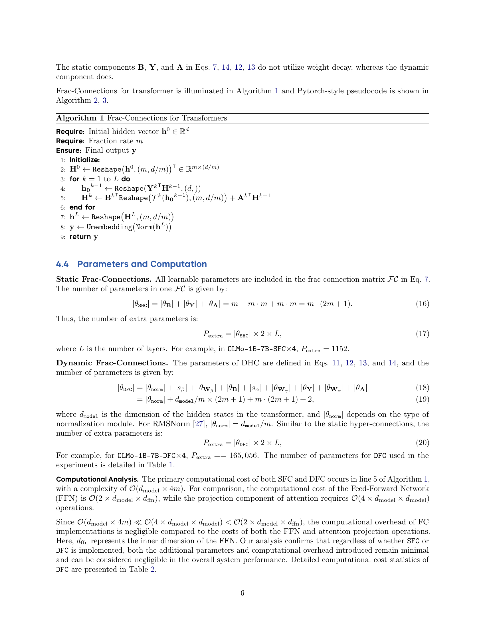
🔼 This table presents a comparison of the total number of parameters across different model configurations. It shows the number of parameters added by the Frac-Connections (FC) method and the resulting total number of parameters in the model. The percentage change in the total number of parameters due to the addition of FC is also provided for each model.
read the caption
Table 1: Comparison of number of parameters.
In-depth insights#
Frac-Connections#
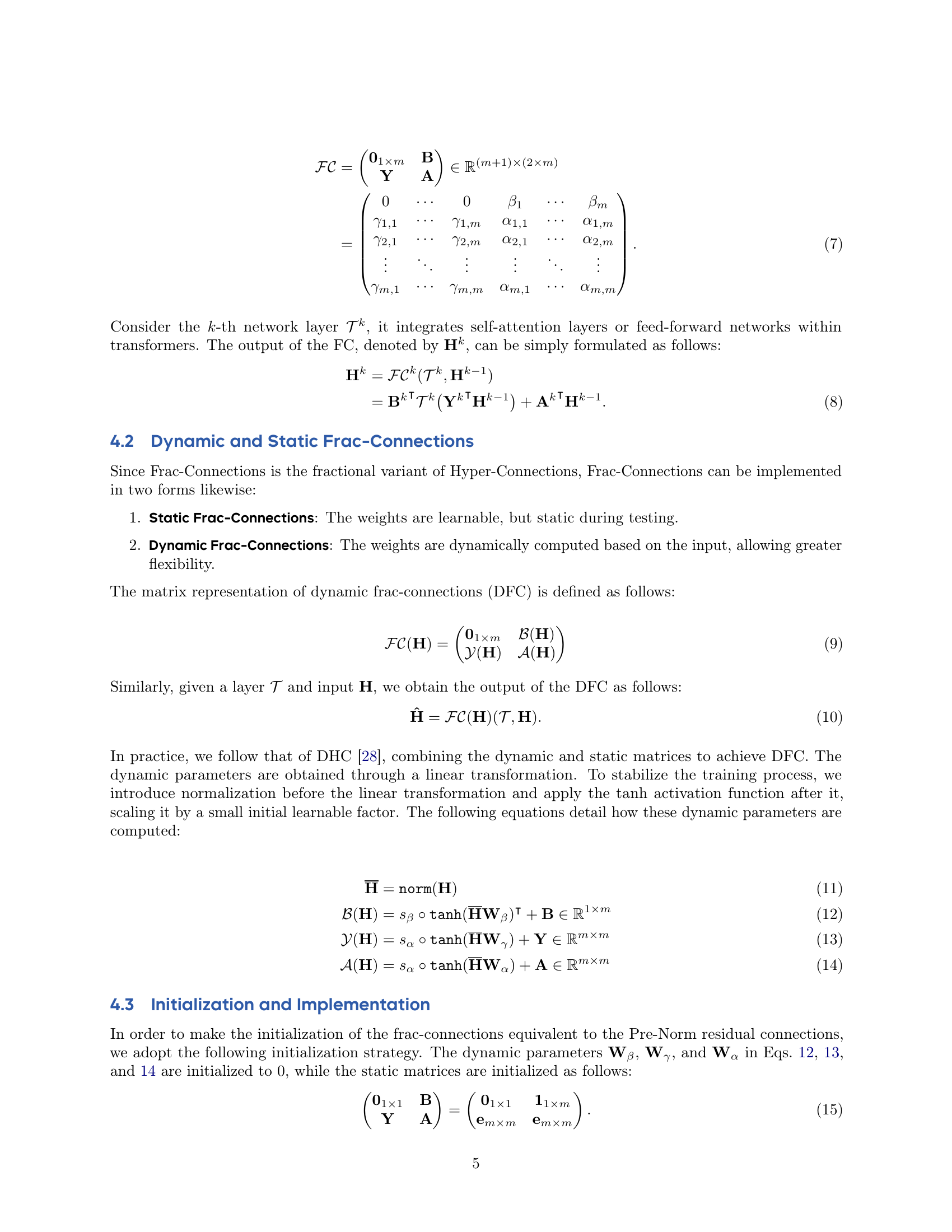
Frac-Connections offer a novel approach to deep learning by dividing hidden states into multiple fractions, unlike Hyper-Connections which expand their width. This method aims to retain benefits of Hyper-Connections, like mitigating gradient vanishing and representational collapse, while reducing memory consumption. Frac-Connections process each fraction independently, potentially allowing for more efficient modeling of complex relationships within the data. The design incorporates learnable scalars or network-predicted values similar to Hyper-Connections, with fractions concatenated after processing and integrated back into the main network. This architecture could offer a sweet spot between residual connections and Hyper-Connections, balancing representational capacity with computational efficiency, potentially leading to improved performance in large-scale language tasks and other domains.
Memory-Efficient#
In the context of research papers, particularly those dealing with deep learning, “Memory-Efficient” would likely address strategies to reduce the computational resources required for training and deploying models. This might involve techniques like quantization, pruning, or knowledge distillation, where the goal is to compress models without significant performance degradation. The paper could explore novel architectures or algorithms that inherently require fewer parameters or memory accesses. The discussion would delve into trade-offs between memory footprint, computational speed, and accuracy, analyzing how various methods impact these factors. Furthermore, it might analyze memory access patterns to optimize data loading and processing, potentially employing techniques like gradient checkpointing to reduce memory usage during backpropagation. The paper might highlight the importance of memory efficiency for deployment on resource-constrained devices or for scaling training to larger datasets and models.
Dynamic Weights#
Dynamic weighting schemes offer a sophisticated approach to adapting model behavior based on input characteristics or training progress. The core idea revolves around assigning varying importance to different components or connections within a network. This adaptability can lead to improved performance, robustness, and generalization. For instance, dynamically adjusting connection weights based on the input hidden state allows the network to prioritize relevant information and suppress noise, akin to an attention mechanism. Similarly, dynamically scaling loss terms during training can focus the model on challenging examples or mitigate imbalances in the dataset. Another avenue is to dynamically modify the learning rate for individual parameters or layers. The efficacy of dynamic weighting hinges on the design of appropriate mechanisms for modulating the weights and the computational cost of implementing these schemes. If designed well, dynamic weighting significantly enhances model capabilities.
Large LLM Impact#
Large language models (LLMs) have revolutionized various fields, showcasing remarkable capabilities in natural language processing. Their impact extends to code generation, creative writing, and question answering. LLMs facilitate enhanced automation and more intuitive human-computer interactions, streamlining workflows and improving accessibility. However, their deployment raises concerns about potential biases, ethical considerations, and misinformation. Responsible development and deployment strategies are crucial to mitigate these risks and ensure LLMs serve as valuable tools for societal benefit, promoting fairness and accuracy in their applications while addressing concerns about job displacement.
Beyond Residuals#
Venturing beyond residual connections in deep learning signifies a quest to overcome inherent limitations like the trade-off between gradient flow and feature redundancy. Innovations could explore alternative skip-connection strategies or entirely new architectural motifs that facilitate more efficient information propagation and representation learning. Attention mechanisms or hyper-networks may be integrated to dynamically modulate connections and optimize information flow, thus enhancing model expressiveness and generalization. Additionally, new normalization techniques can dynamically adjust the weights.
More visual insights#
More on figures

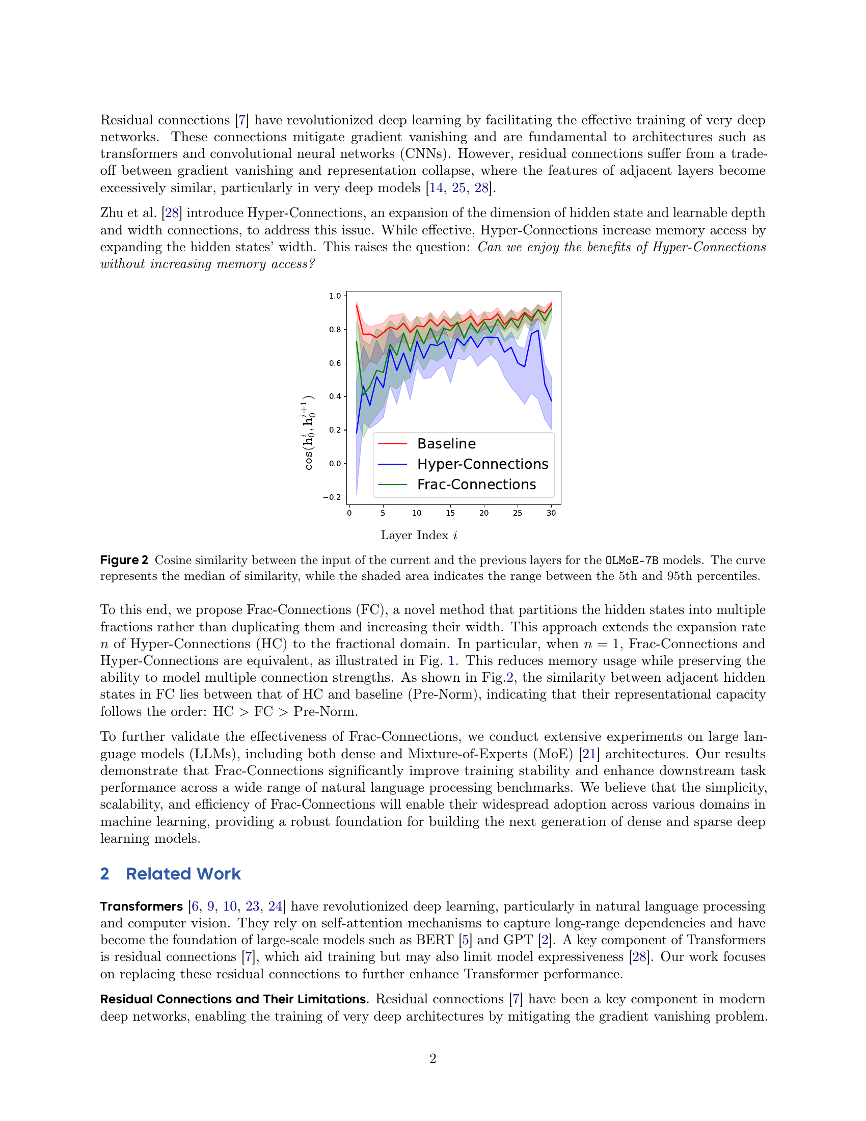
🔼 Figure 2 shows the cosine similarity between the input of each layer and its previous layer for three OLMoE-7B models: a baseline model, a model with Hyper-Connections, and a model with Frac-Connections. The x-axis represents the layer index, and the y-axis represents the cosine similarity. The solid line represents the median cosine similarity, while the shaded area shows the interquartile range (IQR), which is the range between the 5th and 95th percentiles of the cosine similarity. This visualization demonstrates how the different connection methods influence the similarity between adjacent layers. Lower similarity is desirable because it indicates more diverse representations between adjacent layers, which can help to avoid representation collapse.
read the caption
Figure 2: Cosine similarity between the input of the current and the previous layers for the OLMoE-7B models. The curve represents the median of similarity, while the shaded area indicates the range between the 5th and 95th percentiles.

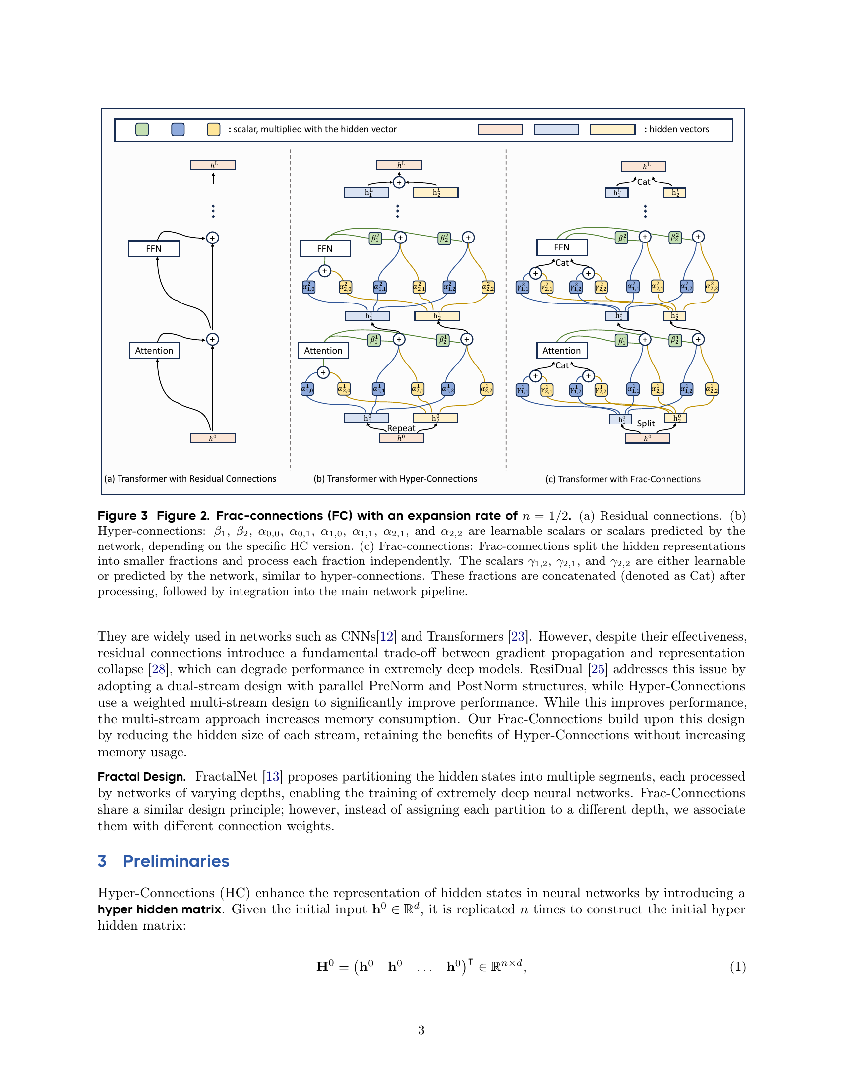
🔼 This figure compares residual connections, hyper-connections, and the proposed frac-connections. Panel (a) shows a standard residual connection. Panel (b) illustrates hyper-connections, which introduce multiple learnable scalar weights connecting different depths of the network. Panel (c) presents frac-connections, a modification that divides the hidden states into multiple parts before processing, resulting in a more memory-efficient way to model multiple connection strengths. The learnable parameters are shown in the figure.
read the caption
Figure 3: Figure 2. Frac-connections (FC) with an expansion rate of n=1/2𝑛12n=1/2italic_n = 1 / 2. (a) Residual connections. (b) Hyper-connections: β1subscript𝛽1\beta_{1}italic_β start_POSTSUBSCRIPT 1 end_POSTSUBSCRIPT, β2subscript𝛽2\beta_{2}italic_β start_POSTSUBSCRIPT 2 end_POSTSUBSCRIPT, α0,0subscript𝛼00\alpha_{0,0}italic_α start_POSTSUBSCRIPT 0 , 0 end_POSTSUBSCRIPT, α0,1subscript𝛼01\alpha_{0,1}italic_α start_POSTSUBSCRIPT 0 , 1 end_POSTSUBSCRIPT, α1,0subscript𝛼10\alpha_{1,0}italic_α start_POSTSUBSCRIPT 1 , 0 end_POSTSUBSCRIPT, α1,1subscript𝛼11\alpha_{1,1}italic_α start_POSTSUBSCRIPT 1 , 1 end_POSTSUBSCRIPT, α2,1subscript𝛼21\alpha_{2,1}italic_α start_POSTSUBSCRIPT 2 , 1 end_POSTSUBSCRIPT, and α2,2subscript𝛼22\alpha_{2,2}italic_α start_POSTSUBSCRIPT 2 , 2 end_POSTSUBSCRIPT are learnable scalars or scalars predicted by the network, depending on the specific HC version. (c) Frac-connections: Frac-connections split the hidden representations into smaller fractions and process each fraction independently. The scalars γ1,2subscript𝛾12\gamma_{1,2}italic_γ start_POSTSUBSCRIPT 1 , 2 end_POSTSUBSCRIPT, γ2,1subscript𝛾21\gamma_{2,1}italic_γ start_POSTSUBSCRIPT 2 , 1 end_POSTSUBSCRIPT, and γ2,2subscript𝛾22\gamma_{2,2}italic_γ start_POSTSUBSCRIPT 2 , 2 end_POSTSUBSCRIPT are either learnable or predicted by the network, similar to hyper-connections. These fractions are concatenated (denoted as Cat) after processing, followed by integration into the main network pipeline.

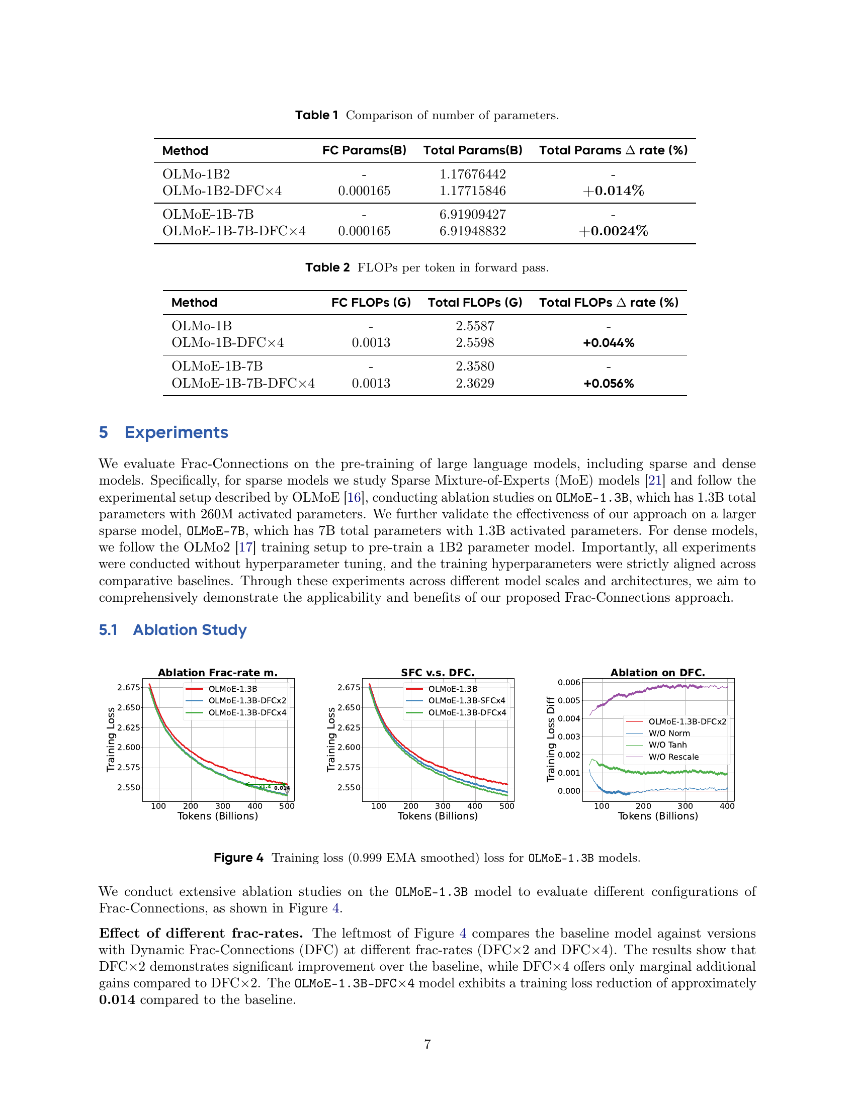
🔼 Figure 4 presents the training loss curves for the OLMoE-1.3B model with various configurations of Frac-Connections. It shows how the loss changes over the course of training (in billions of tokens) for different versions of the model: baseline (no Frac-Connections), Static Frac-Connections (SFC) with different fractional rates (SFCx2 and SFCx4), and Dynamic Frac-Connections (DFC) with different fractional rates (DFCx2 and DFCx4). Additionally, ablation studies are performed on the DFC model by removing normalization, the tanh activation function, or rescaling to analyze the impact of each component on performance. The loss is smoothed using a 0.999 Exponential Moving Average (EMA) filter for better visualization. The purpose of this figure is to demonstrate the improved training stability and efficiency of the Frac-Connection methods compared to the baseline and to understand the role of each component within the DFC model.
read the caption
Figure 4: Training loss (0.999 EMA smoothed) loss for OLMoE-1.3B models.
More on tables
| Method | FC FLOPs (G) | Total FLOPs (G) | Total FLOPs rate (%) |
| OLMo-1B | - | 2.5587 | - |
| OLMo-1B-DFC4 | 0.0013 | 2.5598 | +0.044% |
| OLMoE-1B-7B | - | 2.3580 | - |
| OLMoE-1B-7B-DFC4 | 0.0013 | 2.3629 | +0.056% |
🔼 This table presents the number of floating-point operations (FLOPs) per token during the forward pass of different language models. It compares the FLOPs for the baseline models (OLMO-1B and OLMOE-1B-7B) with those of the models incorporating Frac-Connections (OLMO-1B-DFC×4 and OLMOE-1B-7B-DFC×4). The percentage change in FLOPs after incorporating Frac-Connections is also shown.
read the caption
Table 2: FLOPs per token in forward pass.
| Method |
| BoolQ |
|
| PIQA | SciQ |
| AVG | ||||||||
| OLMoE-7B | 74.28 | 72.87 | 67.64 | 41.83 | 78.73 | 93.60 | 49.14 | 68.30 | ||||||||
| OLMoE-7B-DFC4 | 74.48 | 72.11 | 68.59 | 42.33 | 79.16 | 94.10 | 49.80 | 68.65 |
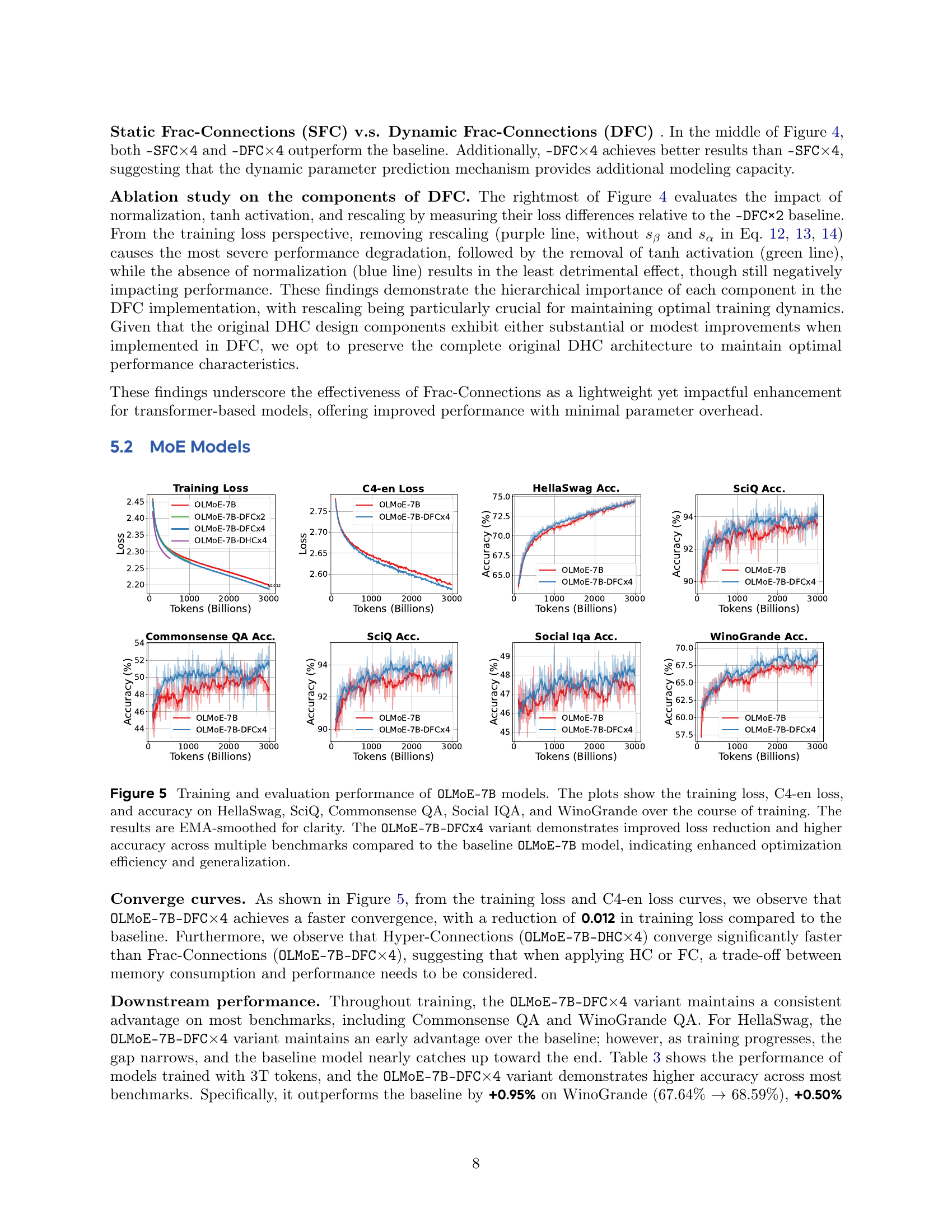
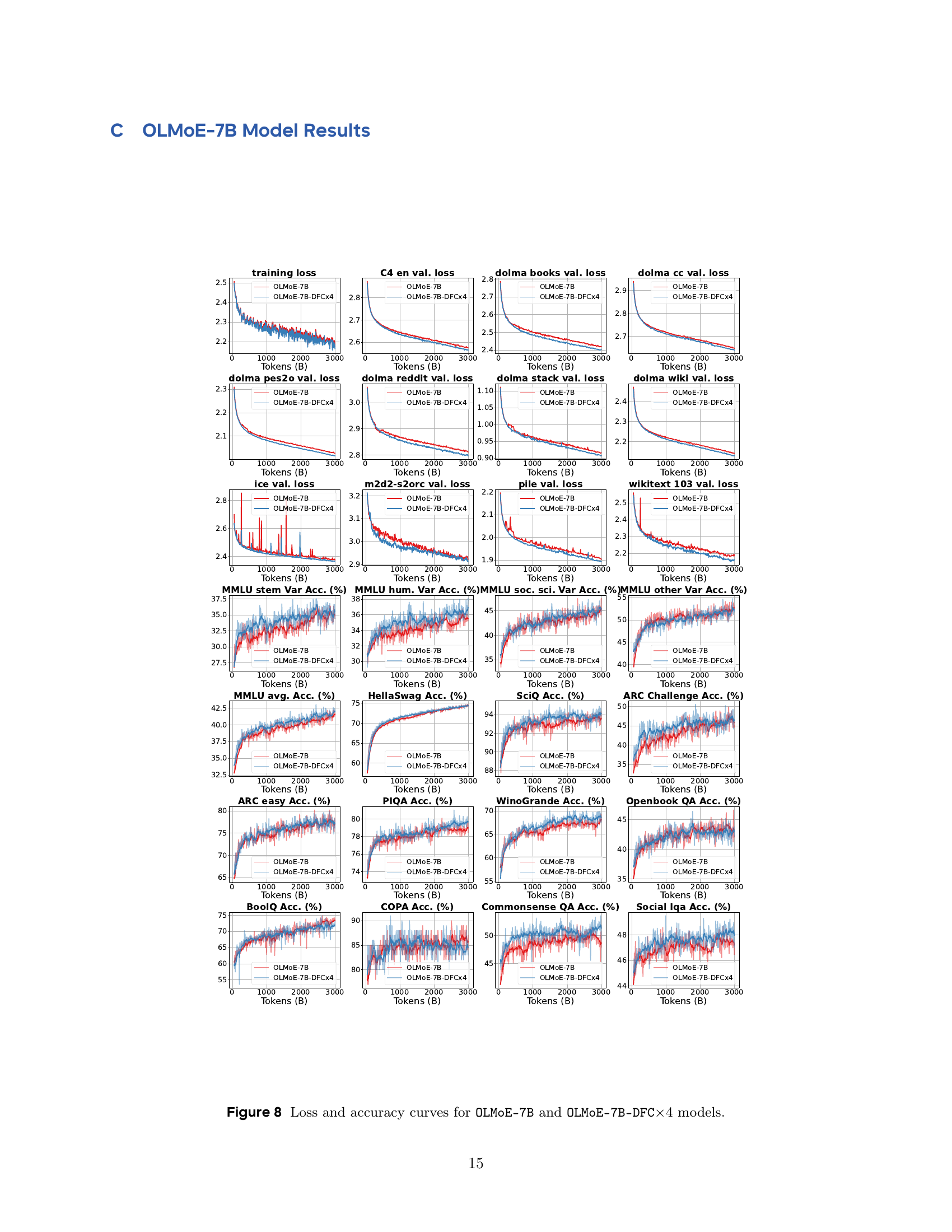
🔼 This table presents the downstream evaluation results for the OLMoE-7B language model after being trained on 3 trillion tokens. It compares the performance of the original OLMoE-7B model against a version incorporating Frac-Connections (OLMoE-7B-DFC×4). The evaluation is performed across multiple benchmarks, including HellaSwag, BoolQ, WinoGrande, MMLU (a modified version with varying few-shot examples for stable early training feedback), PIQA, SciQ, Commonsense QA, and an average score across all benchmarks. The purpose is to demonstrate the impact of Frac-Connections on the model’s performance on diverse downstream tasks.
read the caption
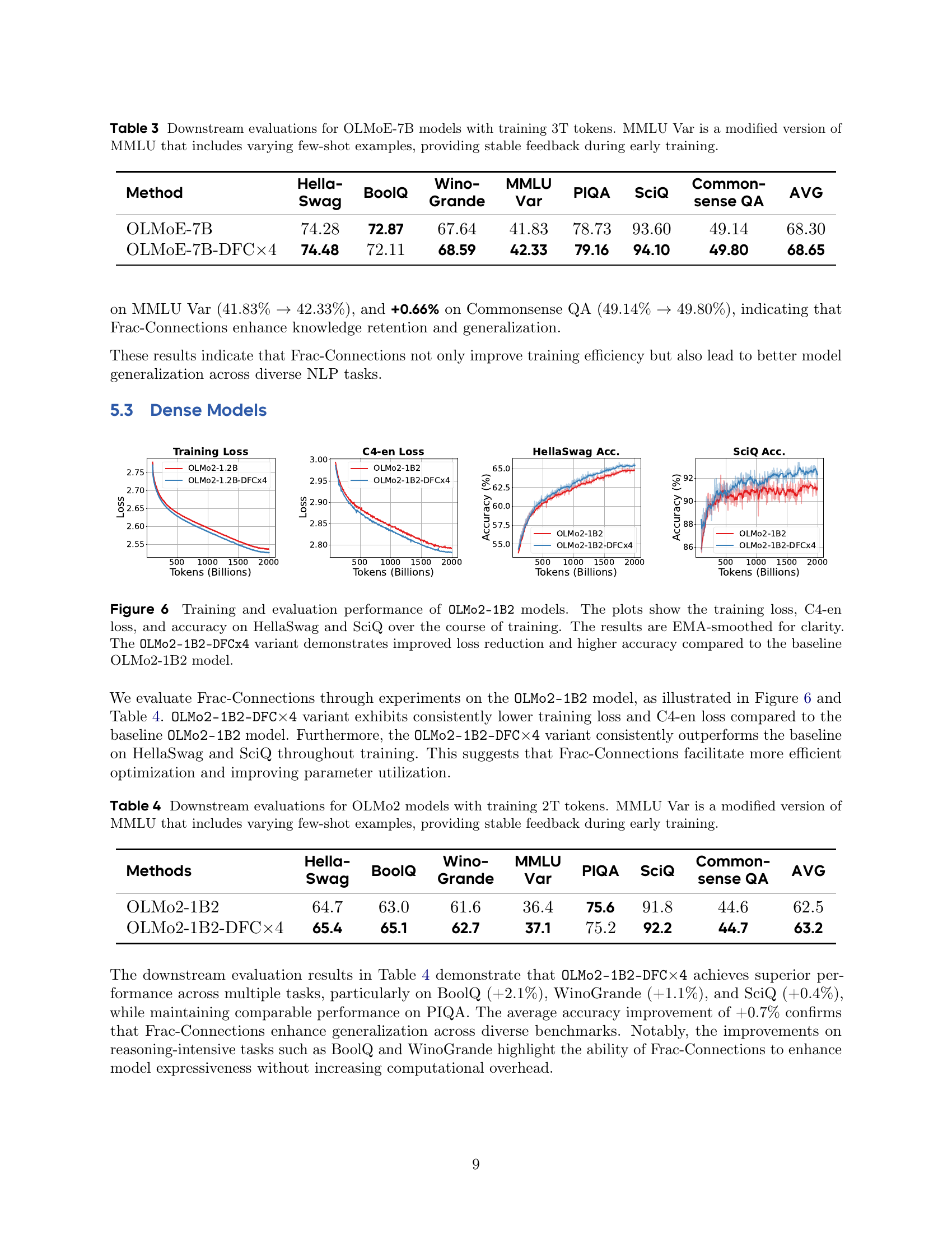
Table 3: Downstream evaluations for OLMoE-7B models with training 3T tokens. MMLU Var is a modified version of MMLU that includes varying few-shot examples, providing stable feedback during early training.
| Hella- |
| Swag |
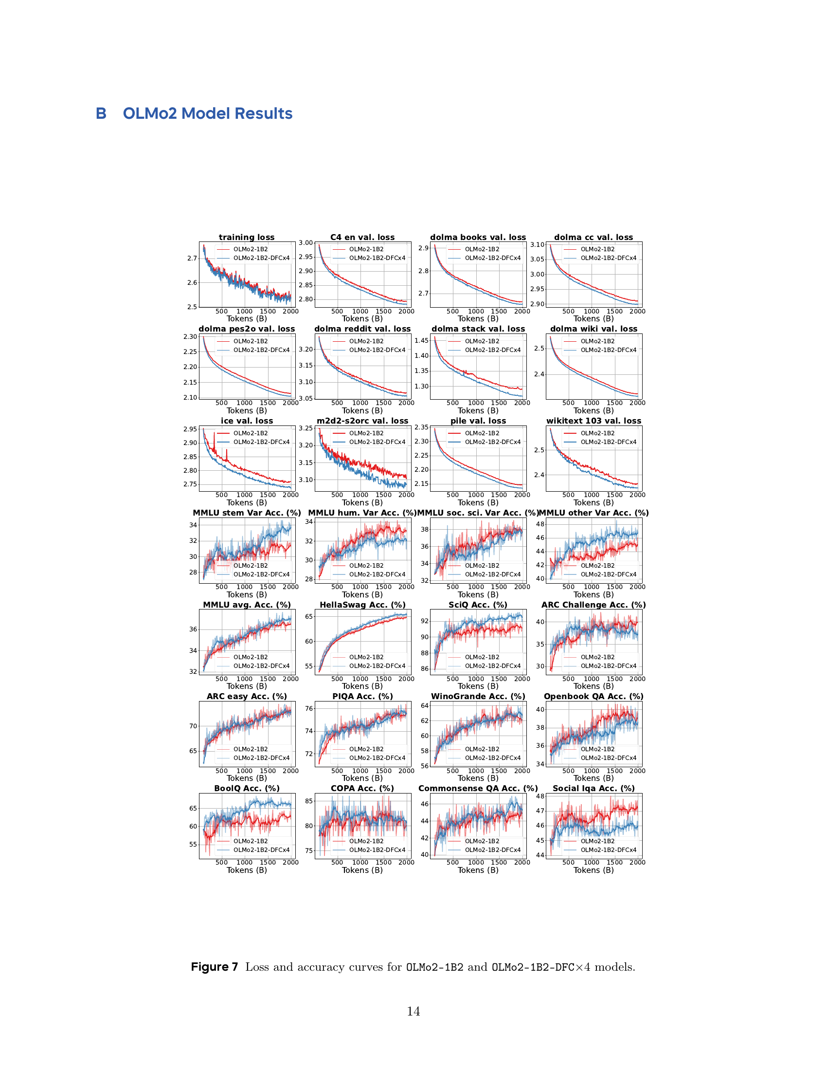
🔼 Table 4 presents the results of downstream evaluations performed on OLMo2 language models. These models were trained using 2 trillion tokens. The table showcases the performance of both the baseline OLMo2-1B2 model and a variant incorporating Dynamic Frac-Connections (OLMo2-1B2-DFC×4). Evaluation metrics include accuracy scores across various benchmarks: HellaSwag, BoolQ, WinoGrande, MMLU Var (a modified version of MMLU with varying few-shot examples for stable early training feedback), PIQA, SciQ, CommonsenseQA, and an average accuracy across all benchmarks. This allows for a direct comparison of the performance improvements achieved by using Dynamic Frac-Connections.
read the caption
Table 4: Downstream evaluations for OLMo2 models with training 2T tokens. MMLU Var is a modified version of MMLU that includes varying few-shot examples, providing stable feedback during early training.
| Wino- |
| Grande |
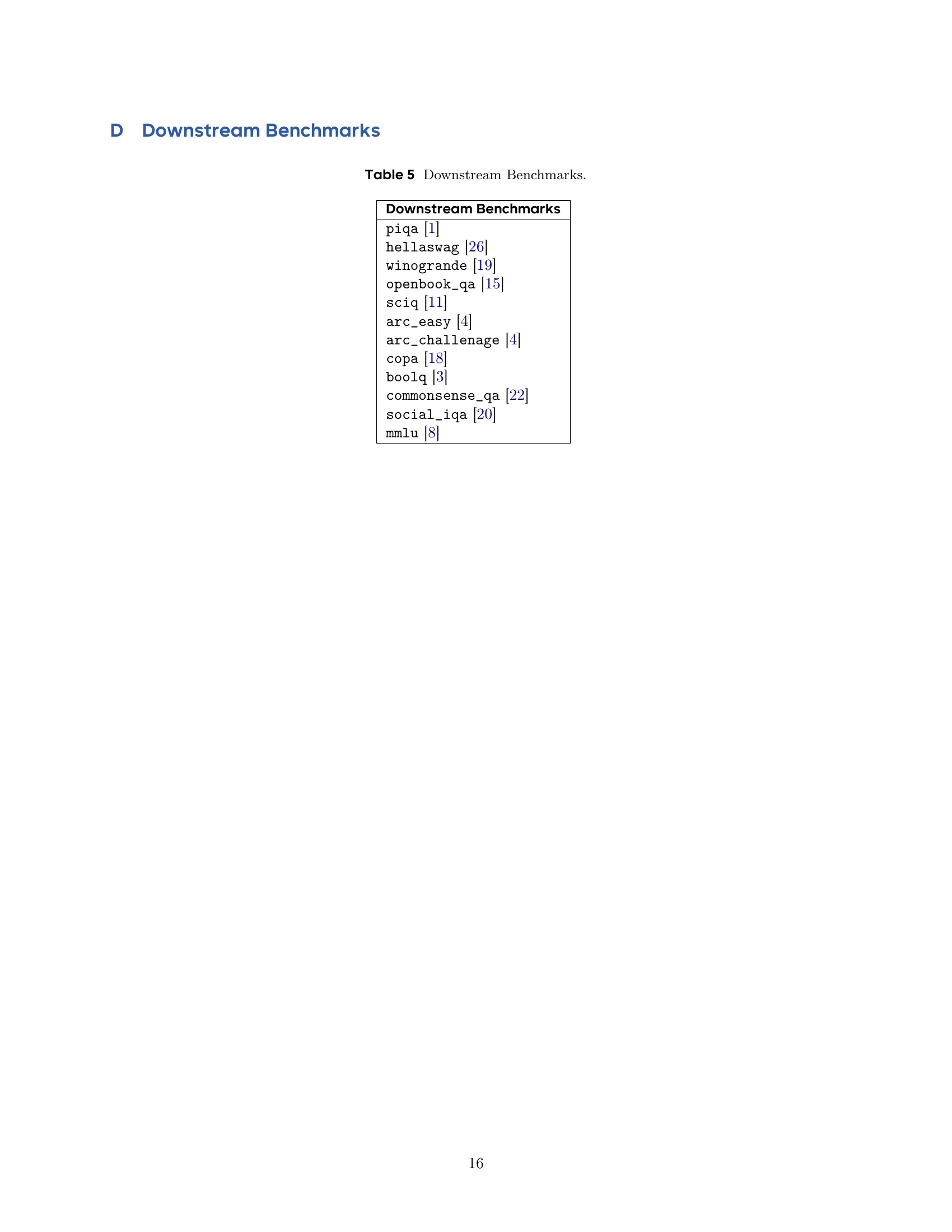
🔼 This table lists the downstream benchmarks used to evaluate the performance of the language models after pre-training. These benchmarks assess various aspects of language understanding and reasoning abilities, including commonsense reasoning, question answering, and factual knowledge.
read the caption
Table 5: Downstream Benchmarks.
Full paper#