TL;DR#
Key Takeaways#
Why does it matter?#
This paper introduces a novel framework for adaptable video models, relevant due to the increasing demand for deployment-efficient solutions in real-world applications. It offers a new perspective on optimizing computation-accuracy trade-offs, and opens avenues for exploring advanced token selection methods, potentially impacting future research in video understanding and multimodal learning.
Visual Insights#

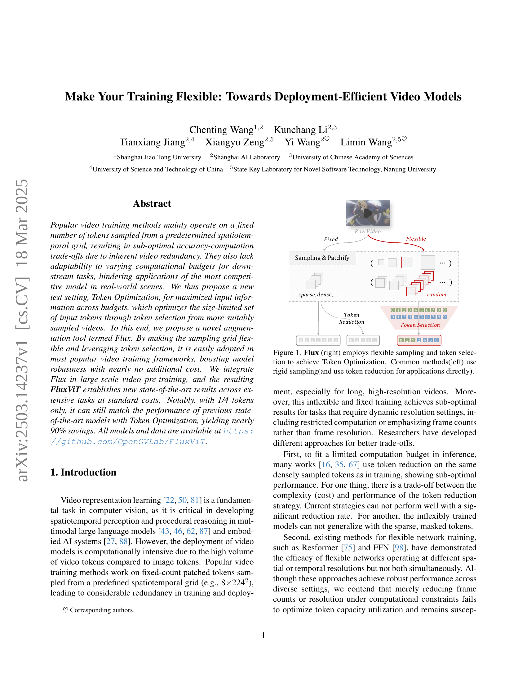
🔼 This figure illustrates the difference between traditional video processing methods and the proposed Flux method. Traditional methods (left) rely on rigid, fixed sampling of video frames, which leads to suboptimal accuracy-computation trade-offs due to redundancy. Token reduction is often employed afterward to reduce computational costs, but this further limits performance. In contrast, the Flux method (right) utilizes flexible sampling and token selection to achieve ‘Token Optimization.’ This involves sampling frames at variable spatiotemporal densities and selecting a size-limited set of tokens that best represent the information within the video. This flexibility allows Flux to adapt better to varying computational budgets and achieve improved accuracy for downstream tasks, especially given limited computational resources.
read the caption
Figure 1: Flux (right) employs flexible sampling and token selection to achieve Token Optimization. Common methods(left) use rigid sampling(and use token reduction for applications directly).
| Method | Input Size | Test Token Number | Avg | |||
| 3072 | 2048 | 1024 | 512 | |||
| 22242 | 69.5 | 69.5 | ||||
| 42242 | 80.5 | 73.6 | 77.1 | |||
| 82242 | 83.9 | 81.9 | 72.7 | 79.5 | ||
| 82242 | 122242 | 84.6 | 84.2 | 80.9 | 69.8 | 79.9 |
| Direct Tuned | 162242 | 84.5 | 83.5 | 79.1 | 67.0 | 78.5 |
| 202242 | 84.1 | 82.7 | 77.7 | 64.3 | 77.2 | |
| 242242 | 83.6 | 82.1 | 76.4 | 62.3 | 76.1 | |
| Avg | 84.2 | 83.3 | 79.4 | 68.5 | - | |
| Max | 84.6 | 84.3 | 81.9 | 73.6 | - | |
| 22242 | 68.1 | 68.1 | ||||
| 42242 | 79.9 | 74.7 | 77.3 | |||
| 82242 | 84.3 | 82.7 | 76.7 | 81.2 | ||
| 122242 | 85.1 | 85.1 | 82.8 | 75.8 | 82.2 | |
| 2048 fixed count | 162242 | 85.4 | 85.2 | 82.6 | 75.3 | 82.1 |
| Flux-Single Tuned | 202242 | 85.6 | 85.1 | 82.2 | 74.6 | 81.9 |
| 242242 | 85.4 | 84.8 | 82.0 | 74.1 | 81.6 | |
| Avg | 85.4 | 84.9 | 82.0 | 74.2 | - | |
| Max | 85.6 | 85.2 | 82.8 | 76.7 | - | |
| 1.0 | 0.9 | 0.9 | 3.1 | - | ||
| 22242 | 69.3 | 69.3 | ||||
| 42242 | 80.5 | 72.8 | 76.7 | |||
| 82242 | 83.9 | 81.9 | 72.7 | 79.5 | ||
| 122242 | 122242 | 85.0 | 84.3 | 80.9 | 67.8 | 79.4 |
| Direct Tuned | 162242 | 84.9 | 83.9 | 78.9 | 65.2 | 78.2 |
| 202242 | 84.7 | 83.4 | 77.6 | 62.4 | 77.0 | |
| 242242 | 84.3 | 82.6 | 76.4 | 60.4 | 75.9 | |
| Avg | 84.7 | 83.6 | 79.4 | 67.2 | - | |
| Max | 85.0 | 84.3 | 81.9 | 72.8 | - | |
| 22242 | 72.2 | 72.2 | ||||
| 42242 | 81.0 | 79.3 | 80.2 | |||
| 82242 | 84.4 | 82.8 | 80.3 | 82.5 | ||
| 122242 | 85.4 | 85.2 | 83.3 | 79.9 | 83.5 | |
| (3072, 2048, 1024) | 162242 | 85.7 | 85.1 | 83.5 | 79.2 | 83.4 |
| Flux-Multi Tuned | 202242 | 85.7 | 85.3 | 83.0 | 78.9 | 83.2 |
| 242242 | 85.6 | 85.0 | 82.7 | 78.2 | 82.9 | |
| Avg | 85.6 | 85.0 | 82.7 | 78.3 | - | |
| Max | 85.7 | 85.3 | 83.5 | 80.3 | - | |
| 0.7 | 1.0 | 1.6 | 7.5 | - | ||
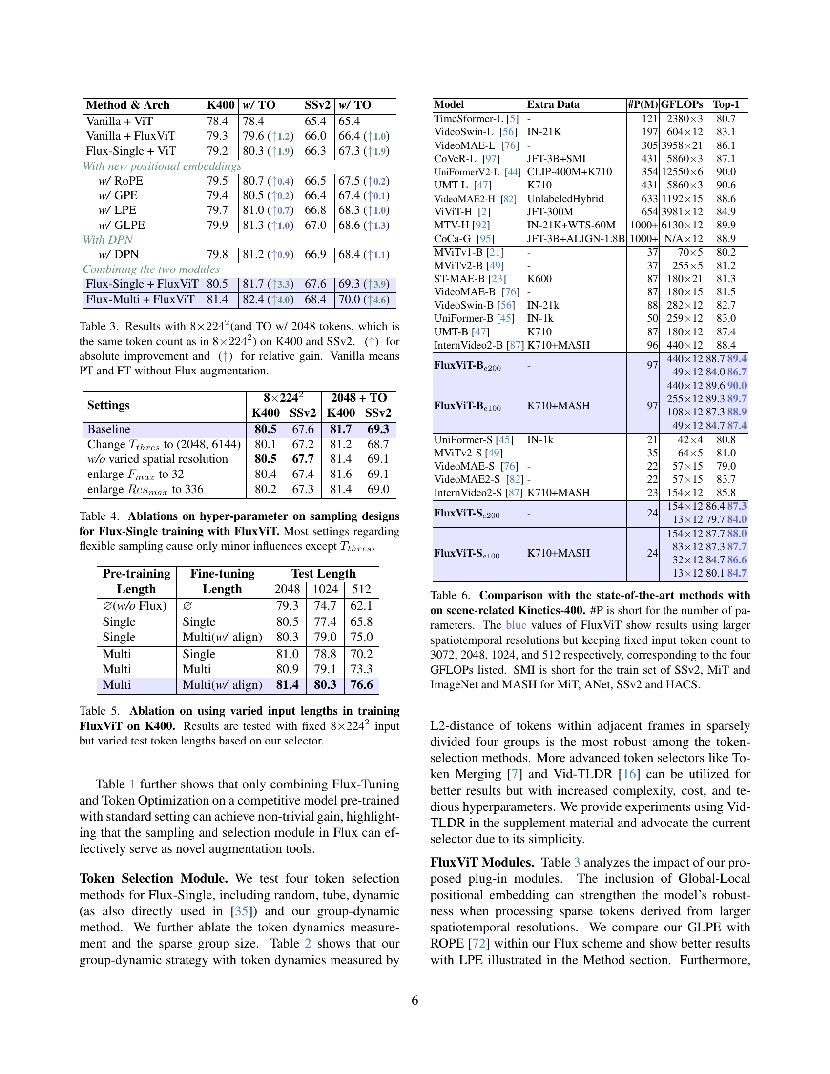
🔼 This table presents the results of applying Flux-Tuning, a novel video augmentation method, directly to the state-of-the-art InternVideo2-S model on the K400 dataset. The experiment evaluates the model’s performance on the K400 dataset using different input sizes (e.g., 2x224², 4x224², etc.) with a fixed token count and compares it to the performance of a directly tuned InternVideo2-S model. The results demonstrate that Flux acts as an advanced augmentation technique, enhancing the performance of the pre-trained model through flexible sampling and token selection, and further improving results through the optimization of the test-time token selection process. Results are reported using a 1clip x 1crop evaluation setting, which shows consistent improvements across input settings.
read the caption
Table 1: Directly use Flux-Tuning with the previsou SOTA InternVideo2-S on K400. Results are reported on K400 using 1clip×\times×1crop. It shows that Flux can be used as an advanced augmentation tool directly in supervised tuning scenario.
In-depth insights#
Flexible Token#
The concept of a “Flexible Token” represents a pivotal shift in how video models are trained and deployed. Traditional methods rely on a fixed number of tokens, sampled from a predetermined grid, which often leads to suboptimal accuracy-computation trade-offs. Flexible tokens aim to address this by allowing the model to adapt to varying computational budgets and downstream task requirements. This adaptability is achieved through techniques such as token selection, where the most informative tokens are prioritized, and flexible sampling, where the sampling grid is adjusted based on the available resources. By embracing flexibility, models can achieve better performance with fewer tokens, leading to deployment-efficient solutions that are suitable for real-world applications with limited computational resources and diverse operational constraints. This represents a move towards more robust and adaptable video understanding systems.
Flux: Key Augment#
Flux fundamentally alters video model training. By introducing flexible sampling and token selection, it allows models to adapt to varying computational budgets, addressing a critical limitation of fixed-grid approaches. This flexibility enhances robustness and efficiency, enabling models to capture more relevant information with fewer tokens. The key insight is that not all tokens are equally important, and a smart selection process can significantly improve performance while reducing computational costs. This augmentation strategy can be integrated into existing frameworks, improving training efficiency and deployment adaptability in real-world applications.
Token Optimize#
Token Optimization, as presented, is a novel perspective focusing on maximizing information gleaned from input tokens given computational constraints. It advocates for intelligently selecting a subset of tokens from videos, rather than relying on a fixed, predefined sampling grid. This approach seeks to address the inherent redundancy in video data and enhance adaptability to varying computational budgets. The core idea revolves around optimizing the choice of input tokens to achieve the best trade-off between computational cost and accuracy. Flexible sampling is promoted, using denser sampling for higher computation and sparser sampling for lower budgets, further enabling spatial and temporal trade-offs. This dynamic adjustment of token selection offers a pathway to more efficient and robust video processing, particularly in resource-constrained deployment scenarios. The approach differs from existing methods, which often apply token reduction techniques after dense sampling. It enhances model generalization by exposing it to a wider range of sparse, masked tokens, improving performance and robustness across diverse settings.
FluxViT: SOTA#
While the paper doesn’t explicitly have a section titled ‘FluxViT: SOTA’, the results presented showcase FluxViT’s state-of-the-art performance across various video understanding tasks. The model achieves competitive accuracy on Kinetics-400, SSv2, and COIN datasets, often surpassing existing methods with significantly reduced computational cost, demonstrating efficient token utilization. Ablation studies validate the effectiveness of Flux’s core components like flexible sampling and the group-dynamic token selector, establishing FluxViT as a highly competitive approach for deployment-efficient video models.
Chat-Centric ViT#
While “Chat-Centric ViT” isn’t a direct heading, we can infer its purpose from the broader context of deployment-efficient video models. It likely refers to adapting Vision Transformers (ViTs) specifically for video understanding within a conversational AI framework. This involves optimizing ViTs for tasks like video captioning, question answering about video content, or enabling a chat assistant to reason about video scenes. Key optimizations might focus on reducing computational cost to enable real-time interaction, such as through token selection strategies as discussed elsewhere in the paper. Furthermore, adapting ViTs for this setting may also require incorporating cross-modal learning approaches to align video features with language embeddings to enable effective interactions. Performance on metrics like MVbench and Dream1k should improve. Finally, it necessitates training strategies emphasizing the relevance and coherence of video-related textual responses to ensure a natural and informative conversational experience.
More visual insights#
More on figures

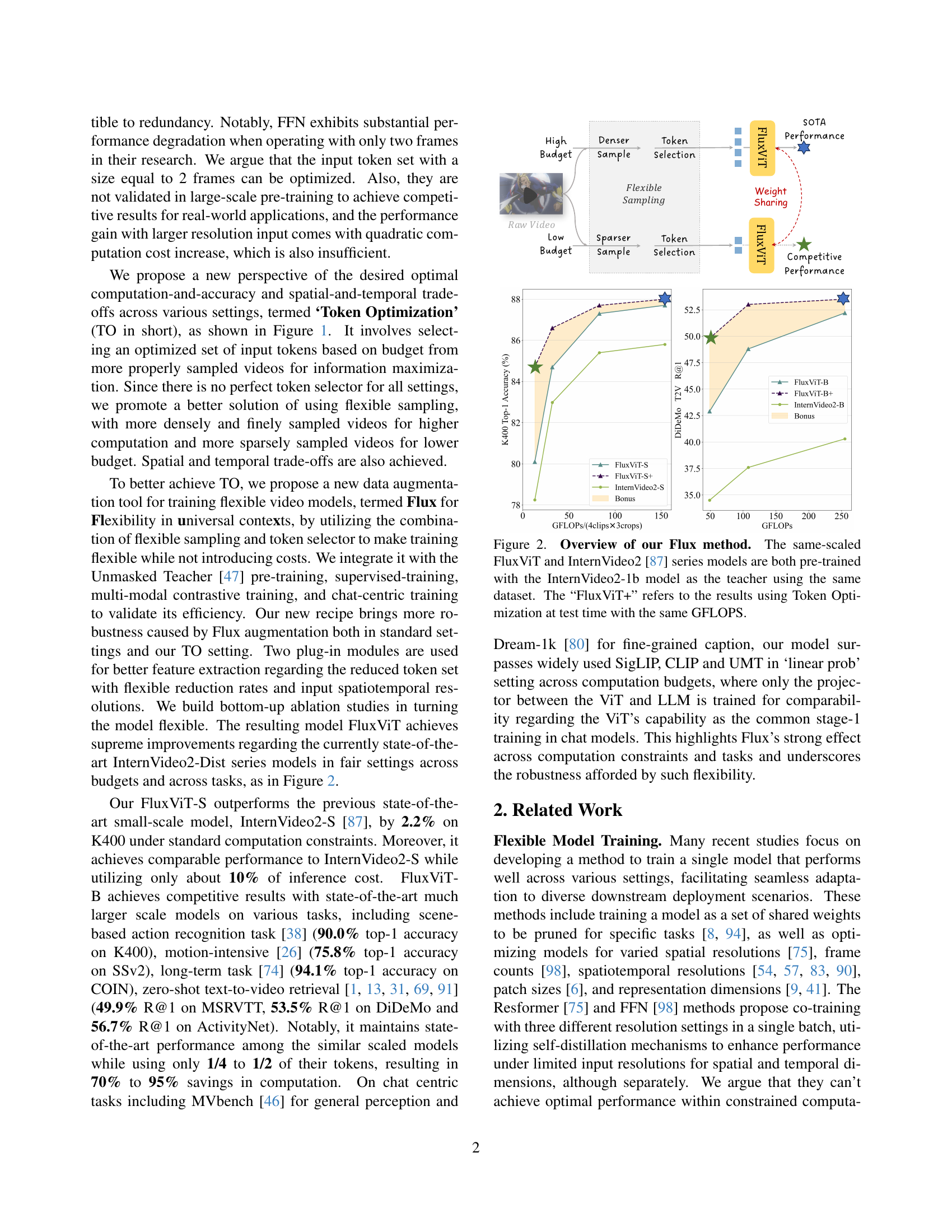
🔼 Figure 2 presents a comparison of the performance between FluxViT and InternVideo2 models. Both models were pre-trained using the same InternVideo2-1b model as a teacher and the same dataset. The key difference is that FluxViT incorporates the proposed Flux method, which enables flexible sampling and token selection. The chart showcases the performance of both models at different computational budgets (GFLOPs). The ‘FluxViT+’ line represents the results when using Token Optimization during the testing phase to optimize the selected input tokens within the same GFLOPs constraint, highlighting the effectiveness of Flux in optimizing video models for resource-constrained settings.
read the caption
Figure 2: Overview of our Flux method. The same-scaled FluxViT and InternVideo2 [87] series models are both pre-trained with the InternVideo2-1b model as the teacher using the same dataset. The “FluxViT+” refers to the results using Token Optimization at test time with the same GFLOPS.

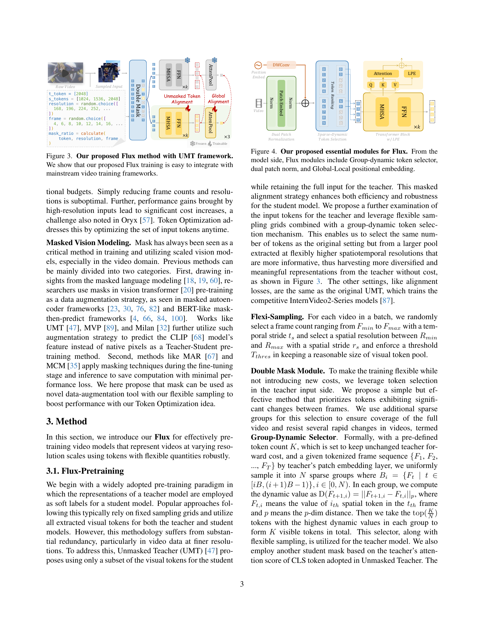
🔼 This figure illustrates how the proposed Flux method integrates with the Unmasked Teacher (UMT) framework for video training. Flux introduces flexible sampling and token selection to address the computational redundancy in standard video models. The diagram shows how a raw video is processed through flexible sampling with varying frame counts and resolutions, followed by token selection to produce a reduced set of tokens. These tokens are then fed into the UMT framework, enabling training of more efficient video models. The figure highlights the ease of integrating Flux into existing video training pipelines.
read the caption
Figure 3: Our proposed Flux method with UMT framework. We show that our proposed Flux training is easy to integrate with mainstream video training frameworks.

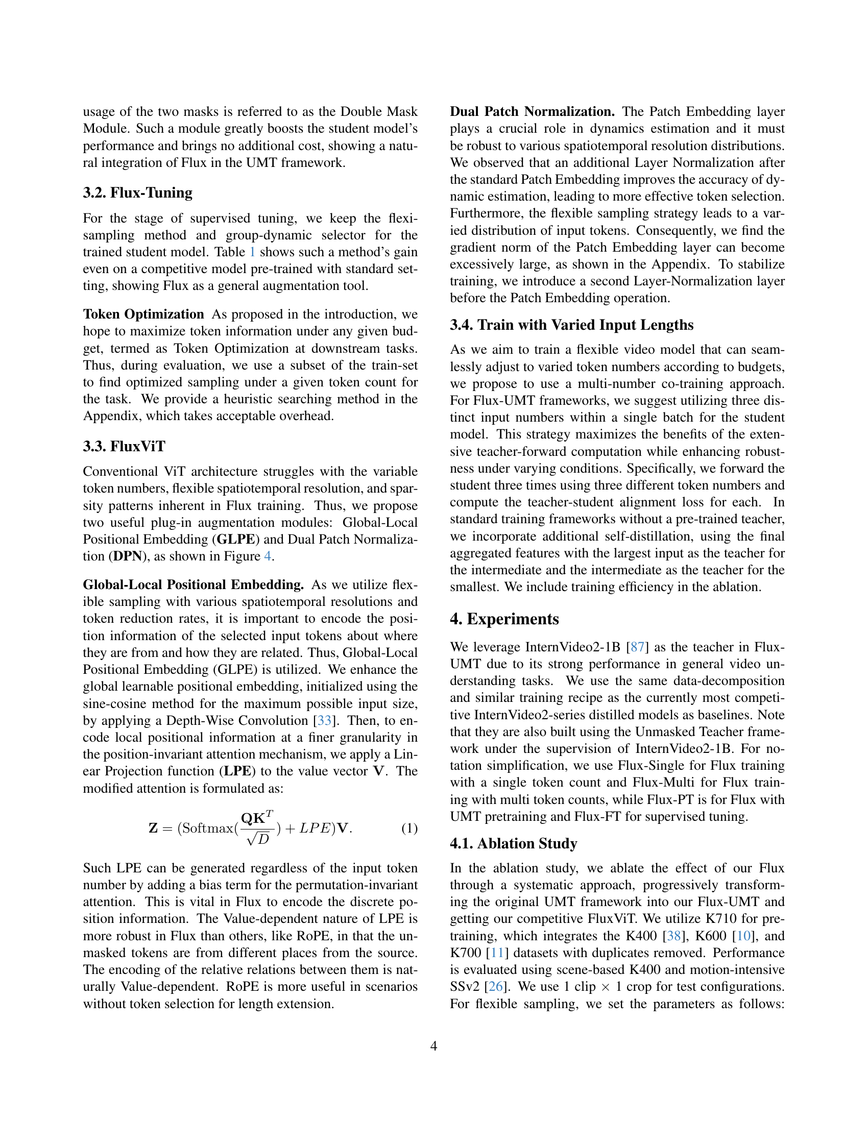
🔼 Figure 4 illustrates the core components of the Flux module, a novel data augmentation technique designed to enhance the flexibility of video models during training. The Flux module consists of three key components: a Group-dynamic token selector which intelligently selects a subset of the most informative tokens from the input video; dual patch normalization which enhances the robustness of the patch embedding process across varying resolutions; and a Global-Local positional embedding method that incorporates both global and fine-grained positional information to handle the variable token lengths and resolutions inherent in the flexible sampling process.
read the caption
Figure 4: Our proposed essential modules for Flux. From the model side, Flux modules include Group-dynamic token selector, dual patch norm, and Global-Local positional embedding.

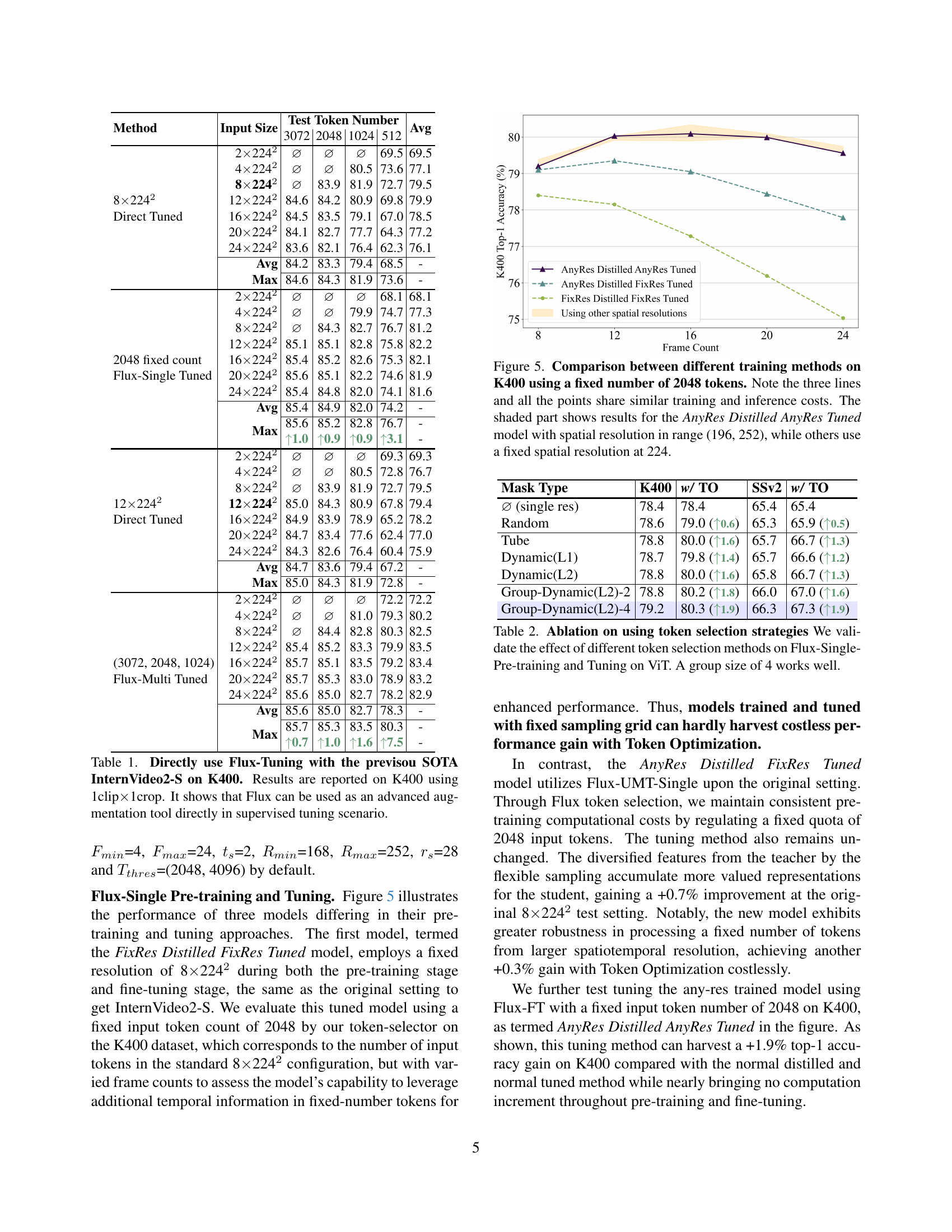
🔼 This figure compares the performance of three different video model training methods on the Kinetics-400 dataset. All methods use a fixed number of 2048 tokens. The x-axis represents the number of frames, and the y-axis represents the top-1 accuracy. The three methods are: 1) FixRes Distilled FixRes Tuned (trained and tested at a fixed spatial resolution of 224); 2) AnyRes Distilled FixRes Tuned (trained at a fixed spatial resolution of 224, but tested at resolutions between 196 and 252); and 3) AnyRes Distilled AnyRes Tuned (trained and tested with spatial resolutions between 196 and 252). The shaded region highlights the performance of the AnyRes Distilled AnyRes Tuned model, demonstrating its superior performance across different frame counts. Notably, all three methods share similar training and inference costs, making this a fair comparison of model training approaches.
read the caption
Figure 5: Comparison between different training methods on K400 using a fixed number of 2048 tokens. Note the three lines and all the points share similar training and inference costs. The shaded part shows results for the AnyRes Distilled AnyRes Tuned model with spatial resolution in range (196, 252), while others use a fixed spatial resolution at 224.

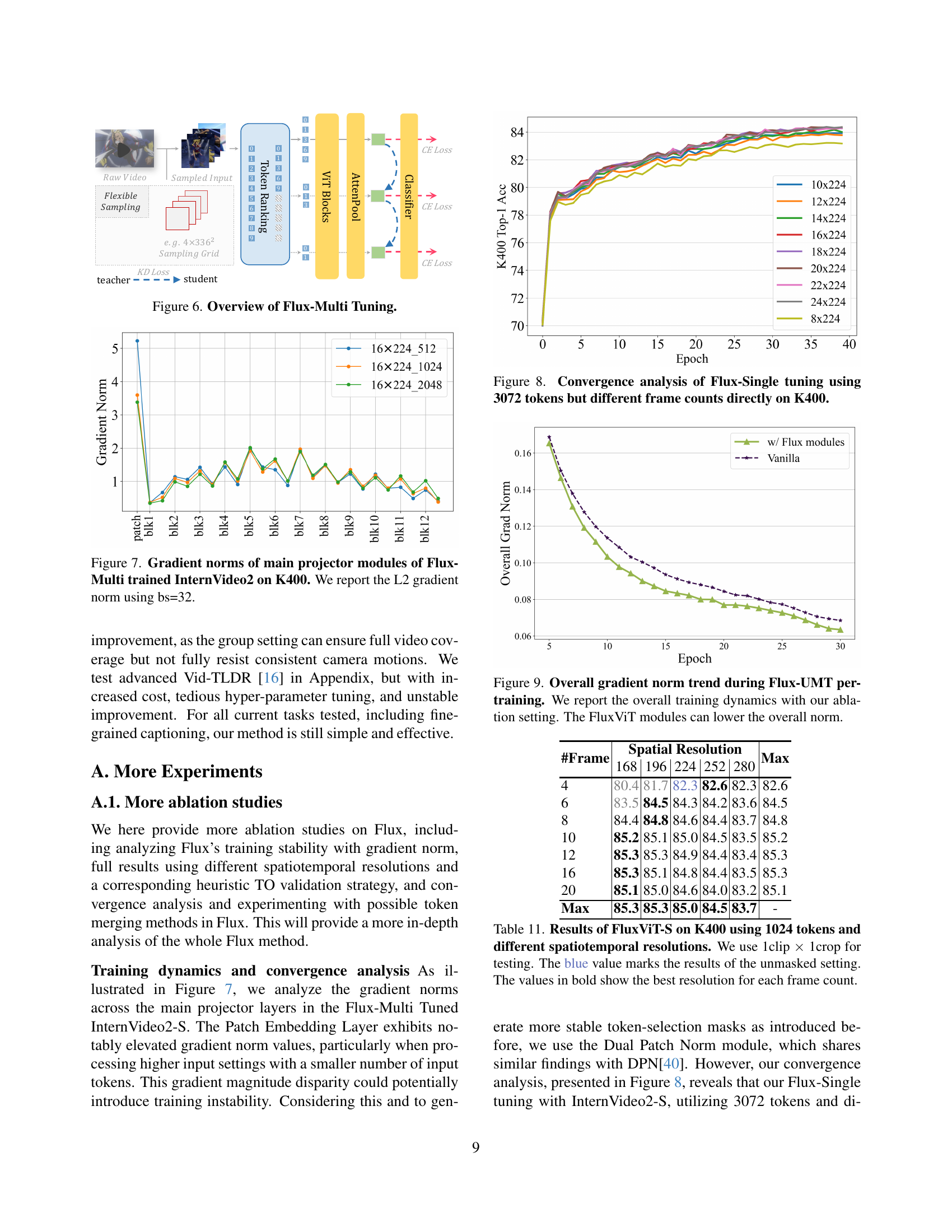
🔼 This figure illustrates the process of Flux-Multi Tuning, a method used to enhance the flexibility and robustness of video models. It shows how multiple token counts are processed concurrently (e.g., 3072, 2048, 1024) within the same training batch. Each token count is processed through the model, and the resulting representations are compared to representations generated from the teacher model using knowledge distillation. This process allows the model to adapt to a wider range of input sizes and computational constraints.
read the caption
Figure 6: Overview of Flux-Multi Tuning.

🔼 This figure visualizes the L2 gradient norms for the main projector modules in the Flux-Multi trained InternVideo2 model, evaluated on the K400 dataset. The batch size (bs) used for the calculation was 32. The plot likely shows the gradient norm across various layers of the network (e.g., different ViT blocks), providing insights into training stability and potential issues like exploding or vanishing gradients. Analyzing gradient norms helps in debugging training processes, assessing the effectiveness of regularization techniques, and understanding the impact of changes in the model architecture, such as those introduced by Flux.
read the caption
Figure 7: Gradient norms of main projector modules of Flux-Multi trained InternVideo2 on K400. We report the L2 gradient norm using bs=32.

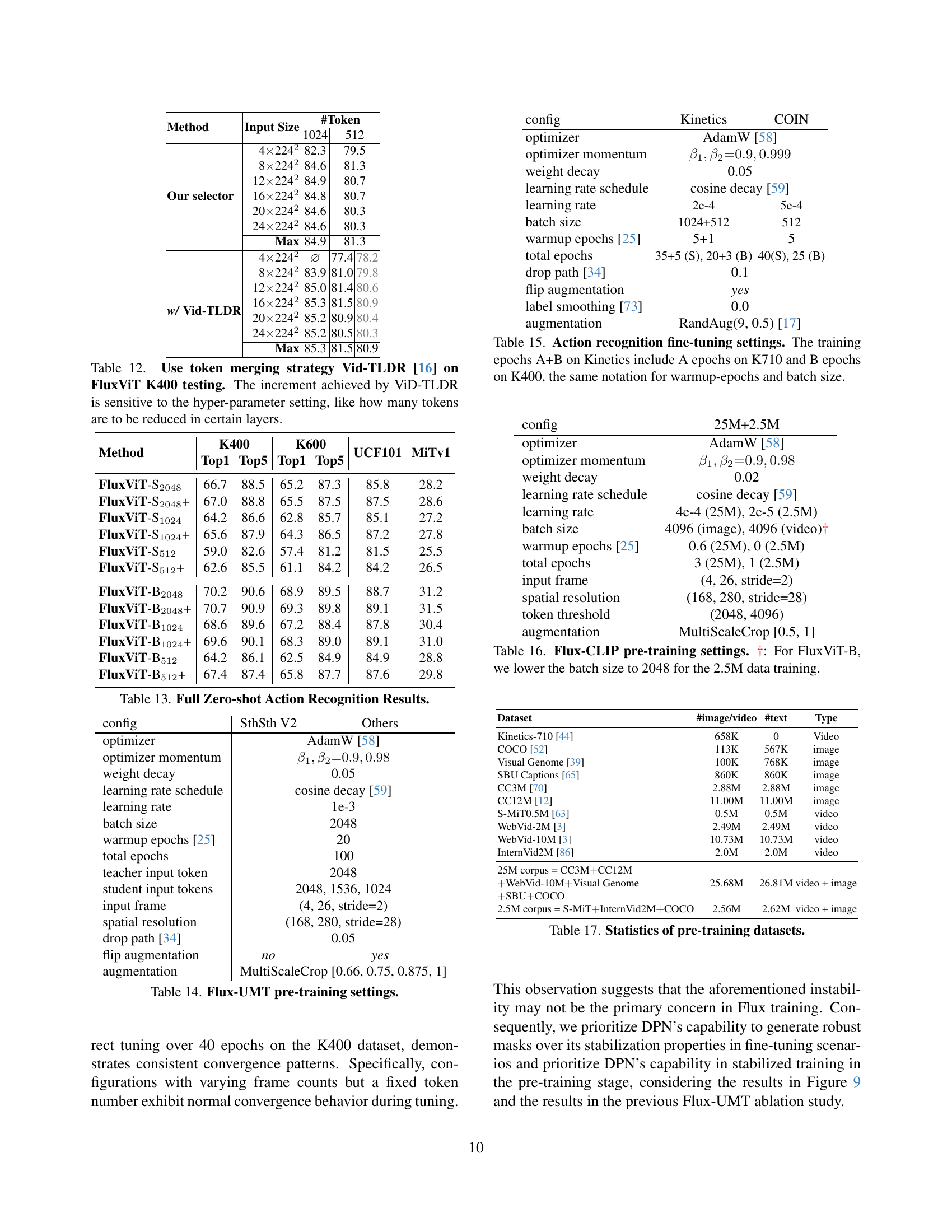
🔼 This figure shows the convergence curves during the fine-tuning stage of the Flux-Single method. The experiment uses a fixed number of 3072 tokens as input for all training runs. However, it varies the number of frames used to generate those tokens, ranging from 10 to 24. The y-axis represents the top-1 accuracy on the K400 dataset, while the x-axis shows the training epoch. The plot visually demonstrates how the model’s performance changes based on different frame counts during training. This helps to analyze the impact of varying the input data’s temporal resolution on the final model accuracy. Different curves represent different number of frames.
read the caption
Figure 8: Convergence analysis of Flux-Single tuning using 3072 tokens but different frame counts directly on K400.

🔼 Figure 9 illustrates the overall gradient norm during the pre-training phase of the Flux-UMT model. The graph plots the gradient norm over training epochs, comparing a standard UMT model to one augmented with the FluxViT modules (Global-Local Positional Embedding and Dual Patch Normalization). The results show that the FluxViT modules contribute to a lower overall gradient norm, indicating improved training stability and potentially better generalization.
read the caption
Figure 9: Overall gradient norm trend during Flux-UMT per-training. We report the overall training dynamics with our ablation setting. The FluxViT modules can lower the overall norm.
More on tables
| Mask Type | K400 | w/ TO | SSv2 | w/ TO |
| (single res) | 78.4 | 78.4 | 65.4 | 65.4 |
| Random | 78.6 | 79.0 (0.6) | 65.3 | 65.9 (0.5) |
| Tube | 78.8 | 80.0 (1.6) | 65.7 | 66.7 (1.3) |
| Dynamic(L1) | 78.7 | 79.8 (1.4) | 65.7 | 66.6 (1.2) |
| Dynamic(L2) | 78.8 | 80.0 (1.6) | 65.8 | 66.7 (1.3) |
| Group-Dynamic(L2)-2 | 78.8 | 80.2 (1.8) | 66.0 | 67.0 (1.6) |
| Group-Dynamic(L2)-4 | 79.2 | 80.3 (1.9) | 66.3 | 67.3 (1.9) |
🔼 This table presents an ablation study evaluating different token selection strategies within the Flux-Single pre-training and tuning method for Vision Transformers (ViTs). The study assesses the impact of various strategies on model performance, comparing random token selection, a tube-based method, and dynamic selection methods using different L1 and L2 norms. The results demonstrate the effectiveness of a group-dynamic selection strategy, specifically with a group size of 4, showing improvements in performance metrics.
read the caption
Table 2: Ablation on using token selection strategies We validate the effect of different token selection methods on Flux-Single-Pre-training and Tuning on ViT. A group size of 4 works well.
| Method & Arch | K400 | w/ TO | SSv2 | w/ TO |
| Vanilla + ViT | 78.4 | 78.4 | 65.4 | 65.4 |
| Vanilla + FluxViT | 79.3 | 79.6 (1.2) | 66.0 | 66.4 (1.0) |
| Flux-Single + ViT | 79.2 | 80.3 (1.9) | 66.3 | 67.3 (1.9) |
| With new positional embeddings | ||||
| w/ RoPE | 79.5 | 80.7 (0.4) | 66.5 | 67.5 (0.2) |
| w/ GPE | 79.4 | 80.5 (0.2) | 66.4 | 67.4 (0.1) |
| w/ LPE | 79.7 | 81.0 (0.7) | 66.8 | 68.3 (1.0) |
| w/ GLPE | 79.9 | 81.3 (1.0) | 67.0 | 68.6 (1.3) |
| With DPN | ||||
| w/ DPN | 79.8 | 81.2 (0.9) | 66.9 | 68.4 (1.1) |
| Combining the two modules | ||||
| Flux-Single + FluxViT | 80.5 | 81.7 (3.3) | 67.6 | 69.3 (3.9) |
| Flux-Multi + FluxViT | 81.4 | 82.4 (4.0) | 68.4 | 70.0 (4.6) |
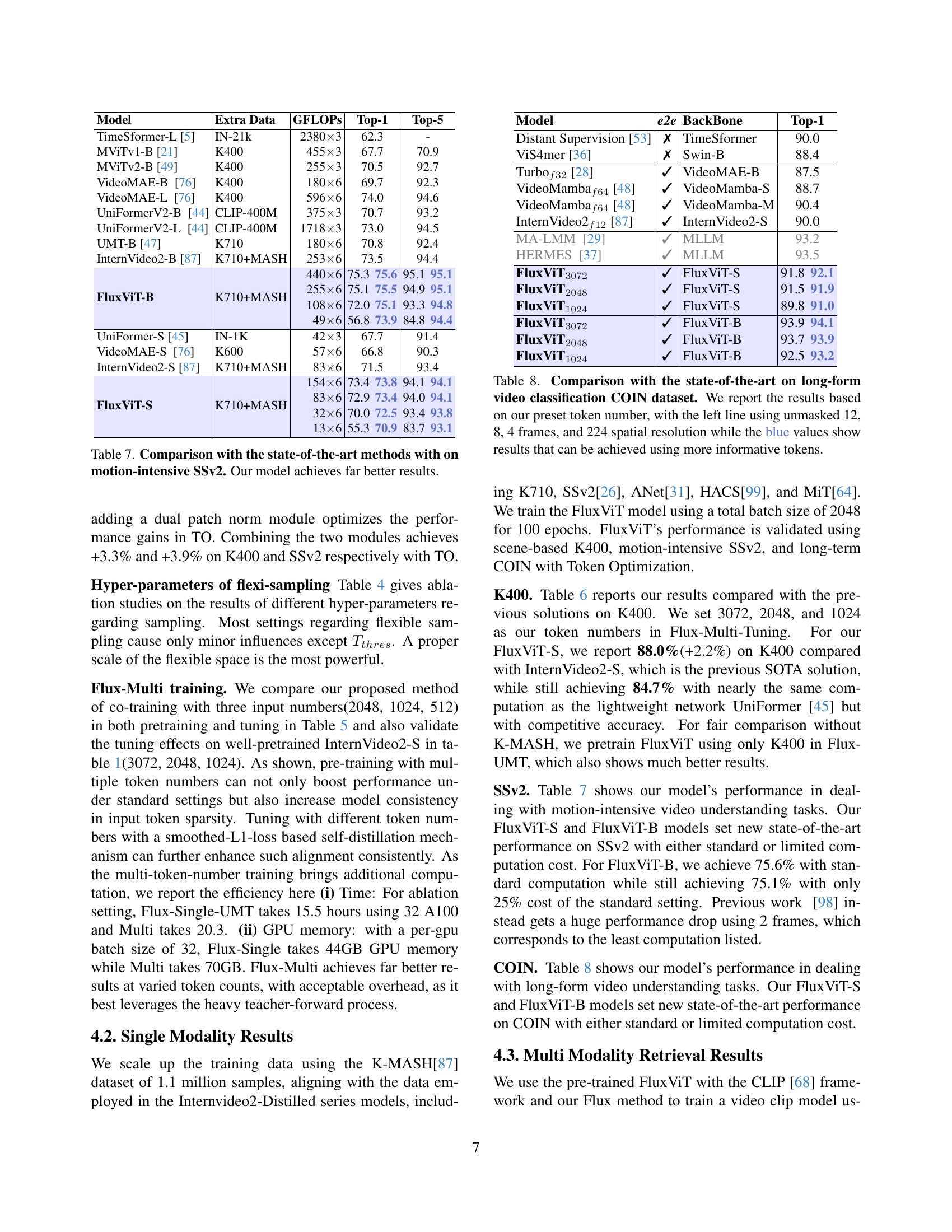
🔼 This table presents a comparison of the performance of various models on the K400 and SSV2 datasets. The models are trained using different methods, including standard training (Vanilla) and training with the proposed Flux method. The table shows the top-1 accuracy for each model, and the absolute and relative improvements achieved by using Flux. The results are presented for models trained with a fixed number of input tokens (2048), equivalent to that produced by a fixed 8x224x224 spatiotemporal grid, for consistent comparison.
read the caption
Table 3: Results with 8×2242absentsuperscript2242\times 224^{2}× 224 start_POSTSUPERSCRIPT 2 end_POSTSUPERSCRIPT(and TO w/ 2048 tokens, which is the same token count as in 8×2242absentsuperscript2242\times 224^{2}× 224 start_POSTSUPERSCRIPT 2 end_POSTSUPERSCRIPT) on K400 and SSv2. (↑↑\uparrow↑) for absolute improvement and (↑↑\uparrow↑) for relative gain. Vanilla means PT and FT without Flux augmentation.
| Settings | 82242 | 2048 + TO | ||
| K400 | SSv2 | K400 | SSv2 | |
| Baseline | 80.5 | 67.6 | 81.7 | 69.3 |
| Change to (2048, 6144) | 80.1 | 67.2 | 81.2 | 68.7 |
| w/o varied spatial resolution | 80.5 | 67.7 | 81.4 | 69.1 |
| enlarge to 32 | 80.4 | 67.4 | 81.6 | 69.1 |
| enlarge to 336 | 80.2 | 67.3 | 81.4 | 69.0 |
🔼 This table presents ablation study results on the hyperparameters used in the flexible sampling process of Flux-Single training with the FluxViT model. The results show the impact of varying several parameters (Fmin, Fmax, ts, Rmin, Rmax, rs, and Tthres) on the model’s performance. It highlights that while many parameters have a minimal effect, the parameter Tthres (a threshold for keeping a reasonable size of the visual token pool) significantly impacts the performance.
read the caption
Table 4: Ablations on hyper-parameter on sampling designs for Flux-Single training with FluxViT. Most settings regarding flexible sampling cause only minor influences except Tthressubscript𝑇𝑡ℎ𝑟𝑒𝑠T_{thres}italic_T start_POSTSUBSCRIPT italic_t italic_h italic_r italic_e italic_s end_POSTSUBSCRIPT.
| Pre-training | Fine-tuning | Test Length | ||||
| Length | Length | 2048 | 1024 | 512 | ||
| (w/o Flux) | 79.3 | 74.7 | 62.1 | |||
| Single | Single | 80.5 | 77.4 | 65.8 | ||
| Single | Multi(w/ align) | 80.3 | 79.0 | 75.0 | ||
| Multi | Single | 81.0 | 78.8 | 70.2 | ||
| Multi | Multi | 80.9 | 79.1 | 73.3 | ||
| Multi | Multi(w/ align) | 81.4 | 80.3 | 76.6 | ||
🔼 This table presents an ablation study on the impact of using varied input lengths during the training of the FluxViT model on the K400 dataset. Specifically, it investigates the effect of varying the number of input tokens at test time while maintaining a fixed input resolution of 8x2242 during training. The table shows the results for different input sizes (2x2242, 4x2242, 8x2242, 12x2242, 16x2242, 20x2242, 24x2242) and various token counts at test time (3072, 2048, 1024, 512). The results are reported in terms of top-1 accuracy on the K400 dataset. This helps to understand how flexible the model is to changes in input length during inference. The table compares the performance of direct tuning (without Flux) and Flux-tuning with both single and multiple input lengths during training.
read the caption
Table 5: Ablation on using varied input lengths in training FluxViT on K400. Results are tested with fixed 8×\times×2242 input but varied test token lengths based on our selector.
| Model | Extra Data | #P(M) | GFLOPs | Top-1 | |
| TimeSformer-L [5] | - | 121 | 23803 | 80.7 | |
| VideoSwin-L [56] | IN-21K | 197 | 60412 | 83.1 | |
| VideoMAE-L [76] | - | 305 | 395821 | 86.1 | |
| CoVeR-L [97] | JFT-3B+SMI | 431 | 58603 | 87.1 | |
| UniFormerV2-L [44] | CLIP-400M+K710 | 354 | 125506 | 90.0 | |
| UMT-L [47] | K710 | 431 | 58603 | 90.6 | |
| VideoMAE2-H [82] | UnlabeledHybrid | 633 | 119215 | 88.6 | |
| ViViT-H [2] | JFT-300M | 654 | 398112 | 84.9 | |
| MTV-H [92] | IN-21K+WTS-60M | 1000+ | 613012 | 89.9 | |
| CoCa-G [95] | JFT-3B+ALIGN-1.8B | 1000+ | N/A12 | 88.9 | |
| MViTv1-B [21] | - | 37 | 705 | 80.2 | |
| MViTv2-B [49] | - | 37 | 2555 | 81.2 | |
| ST-MAE-B [23] | K600 | 87 | 18021 | 81.3 | |
| VideoMAE-B [76] | - | 87 | 18015 | 81.5 | |
| VideoSwin-B [56] | IN-21k | 88 | 28212 | 82.7 | |
| UniFormer-B [45] | IN-1k | 50 | 25912 | 83.0 | |
| UMT-B [47] | K710 | 87 | 18012 | 87.4 | |
| InternVideo2-B [87] | K710+MASH | 96 | 44012 | 88.4 | |
| 44012 | 88.7 | 89.4 | |||
| FluxViT-Be200 | - | 97 | 4912 | 84.0 | 86.7 |
| 44012 | 89.6 | 90.0 | |||
| 25512 | 89.3 | 89.7 | |||
| 10812 | 87.3 | 88.9 | |||
| FluxViT-Be100 | K710+MASH | 97 | 4912 | 84.7 | 87.4 |
| UniFormer-S [45] | IN-1k | 21 | 424 | 80.8 | |
| MViTv2-S [49] | - | 35 | 645 | 81.0 | |
| VideoMAE-S [76] | - | 22 | 5715 | 79.0 | |
| VideoMAE2-S [82] | - | 22 | 5715 | 83.7 | |
| InternVideo2-S [87] | K710+MASH | 23 | 15412 | 85.8 | |
| 15412 | 86.4 | 87.3 | |||
| FluxViT-Se200 | - | 24 | 1312 | 79.7 | 84.0 |
| 15412 | 87.7 | 88.0 | |||
| 8312 | 87.3 | 87.7 | |||
| 3212 | 84.7 | 86.6 | |||
| FluxViT-Se100 | K710+MASH | 24 | 1312 | 80.1 | 84.7 |
🔼 Table 6 presents a comparison of FluxViT’s performance against state-of-the-art models on the scene-related Kinetics-400 dataset. The table highlights the impact of FluxViT’s flexible sampling and token selection strategies by showing results for different model sizes and computational budgets. The key finding is that FluxViT can achieve competitive or superior performance while using significantly fewer tokens than comparable models, demonstrating its efficiency and adaptability. The table includes model name, additional training data used, the number of parameters (#P), GFLOPS (a measure of computational cost), and top-1 accuracy. Blue values for FluxViT indicate results obtained by using higher spatiotemporal resolutions while maintaining a fixed number of input tokens (3072, 2048, 1024, 512), illustrating the model’s flexibility. Abbreviations used: SMI (SSv2, MiT, and ImageNet training data) and MASH (MiT, ANet, SSv2, and HACS training data).
read the caption
Table 6: Comparison with the state-of-the-art methods with on scene-related Kinetics-400. #P is short for the number of parameters. The blue values of FluxViT show results using larger spatiotemporal resolutions but keeping fixed input token count to 3072, 2048, 1024, and 512 respectively, corresponding to the four GFLOPs listed. SMI is short for the train set of SSv2, MiT and ImageNet and MASH for MiT, ANet, SSv2 and HACS.
| Model | Extra Data | GFLOPs | Top-1 | Top-5 | ||
| TimeSformer-L [5] | IN-21k | 23803 | 62.3 | - | ||
| MViTv1-B [21] | K400 | 4553 | 67.7 | 70.9 | ||
| MViTv2-B [49] | K400 | 2553 | 70.5 | 92.7 | ||
| VideoMAE-B [76] | K400 | 1806 | 69.7 | 92.3 | ||
| VideoMAE-L [76] | K400 | 5966 | 74.0 | 94.6 | ||
| UniFormerV2-B [44] | CLIP-400M | 3753 | 70.7 | 93.2 | ||
| UniFormerV2-L [44] | CLIP-400M | 17183 | 73.0 | 94.5 | ||
| UMT-B [47] | K710 | 1806 | 70.8 | 92.4 | ||
| InternVideo2-B [87] | K710+MASH | 2536 | 73.5 | 94.4 | ||
| 4406 | 75.3 | 75.6 | 95.1 | 95.1 | ||
| 2556 | 75.1 | 75.5 | 94.9 | 95.1 | ||
| 1086 | 72.0 | 75.1 | 93.3 | 94.8 | ||
| FluxViT-B | K710+MASH | 496 | 56.8 | 73.9 | 84.8 | 94.4 |
| UniFormer-S [45] | IN-1K | 423 | 67.7 | 91.4 | ||
| VideoMAE-S [76] | K600 | 576 | 66.8 | 90.3 | ||
| InternVideo2-S [87] | K710+MASH | 836 | 71.5 | 93.4 | ||
| 1546 | 73.4 | 73.8 | 94.1 | 94.1 | ||
| 836 | 72.9 | 73.4 | 94.0 | 94.1 | ||
| 326 | 70.0 | 72.5 | 93.4 | 93.8 | ||
| FluxViT-S | K710+MASH | 136 | 55.3 | 70.9 | 83.7 | 93.1 |
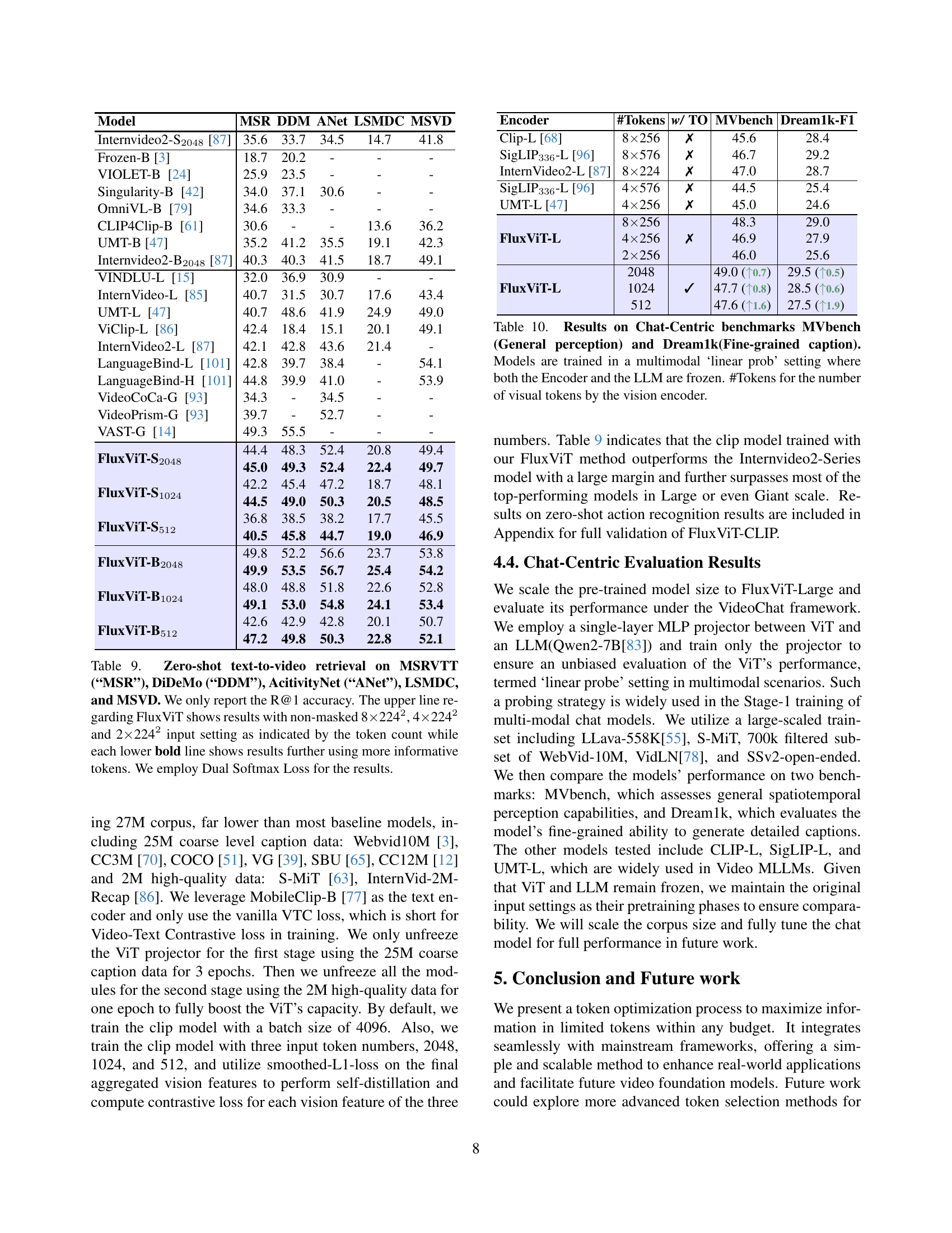
🔼 Table 7 presents a comparison of the proposed FluxViT model’s performance against state-of-the-art methods on the SSv2 dataset, which is specifically designed for motion-intensive video understanding tasks. The table highlights the superior performance of FluxViT, demonstrating its effectiveness in handling challenging video content with significant motion.
read the caption
Table 7: Comparison with the state-of-the-art methods with on motion-intensive SSv2. Our model achieves far better results.
| Model | e2e | BackBone | Top-1 | |
| Distant Supervision [53] | ✗ | TimeSformer | 90.0 | |
| ViS4mer [36] | ✗ | Swin-B | 88.4 | |
| Turbof32 [28] | ✓ | VideoMAE-B | 87.5 | |
| VideoMambaf64 [48] | ✓ | VideoMamba-S | 88.7 | |
| VideoMambaf64 [48] | ✓ | VideoMamba-M | 90.4 | |
| InternVideo2f12 [87] | ✓ | InternVideo2-S | 90.0 | |
| MA-LMM [29] | ✓ | MLLM | 93.2 | |
| HERMES [37] | ✓ | MLLM | 93.5 | |
| FluxViT3072 | ✓ | FluxViT-S | 91.8 | 92.1 |
| FluxViT2048 | ✓ | FluxViT-S | 91.5 | 91.9 |
| FluxViT1024 | ✓ | FluxViT-S | 89.8 | 91.0 |
| FluxViT3072 | ✓ | FluxViT-B | 93.9 | 94.1 |
| FluxViT2048 | ✓ | FluxViT-B | 93.7 | 93.9 |
| FluxViT1024 | ✓ | FluxViT-B | 92.5 | 93.2 |
🔼 Table 8 presents a comparison of the model’s performance on the COIN dataset against state-of-the-art methods for long-form video classification. The results are organized by the number of tokens used and the training strategy. The left column shows results obtained using a standard approach (unmasked 12, 8, and 4 frames at 224 spatial resolution). The blue values represent performance improvements achieved by utilizing a more optimized token selection process, effectively leveraging more informative tokens. This demonstrates the efficacy of the proposed approach in improving performance with the same computational cost.
read the caption
Table 8: Comparison with the state-of-the-art on long-form video classification COIN dataset. We report the results based on our preset token number, with the left line using unmasked 12, 8, 4 frames, and 224 spatial resolution while the blue values show results that can be achieved using more informative tokens.
| Model | MSR | DDM | ANet | LSMDC | MSVD |
| Internvideo2-S2048 [87] | 35.6 | 33.7 | 34.5 | 14.7 | 41.8 |
| Frozen-B [3] | 18.7 | 20.2 | - | - | - |
| VIOLET-B [24] | 25.9 | 23.5 | - | - | - |
| Singularity-B [42] | 34.0 | 37.1 | 30.6 | - | - |
| OmniVL-B [79] | 34.6 | 33.3 | - | - | - |
| CLIP4Clip-B [61] | 30.6 | - | - | 13.6 | 36.2 |
| UMT-B [47] | 35.2 | 41.2 | 35.5 | 19.1 | 42.3 |
| Internvideo2-B2048 [87] | 40.3 | 40.3 | 41.5 | 18.7 | 49.1 |
| VINDLU-L [15] | 32.0 | 36.9 | 30.9 | - | - |
| InternVideo-L [85] | 40.7 | 31.5 | 30.7 | 17.6 | 43.4 |
| UMT-L [47] | 40.7 | 48.6 | 41.9 | 24.9 | 49.0 |
| ViClip-L [86] | 42.4 | 18.4 | 15.1 | 20.1 | 49.1 |
| InternVideo2-L [87] | 42.1 | 42.8 | 43.6 | 21.4 | - |
| LanguageBind-L [101] | 42.8 | 39.7 | 38.4 | - | 54.1 |
| LanguageBind-H [101] | 44.8 | 39.9 | 41.0 | - | 53.9 |
| VideoCoCa-G [93] | 34.3 | - | 34.5 | - | - |
| VideoPrism-G [93] | 39.7 | - | 52.7 | - | - |
| VAST-G [14] | 49.3 | 55.5 | - | - | - |
| 44.4 | 48.3 | 52.4 | 20.8 | 49.4 | |
| FluxViT-S2048 | 45.0 | 49.3 | 52.4 | 22.4 | 49.7 |
| 42.2 | 45.4 | 47.2 | 18.7 | 48.1 | |
| FluxViT-S1024 | 44.5 | 49.0 | 50.3 | 20.5 | 48.5 |
| 36.8 | 38.5 | 38.2 | 17.7 | 45.5 | |
| FluxViT-S512 | 40.5 | 45.8 | 44.7 | 19.0 | 46.9 |
| 49.8 | 52.2 | 56.6 | 23.7 | 53.8 | |
| FluxViT-B2048 | 49.9 | 53.5 | 56.7 | 25.4 | 54.2 |
| 48.0 | 48.8 | 51.8 | 22.6 | 52.8 | |
| FluxViT-B1024 | 49.1 | 53.0 | 54.8 | 24.1 | 53.4 |
| 42.6 | 42.9 | 42.8 | 20.1 | 50.7 | |
| FluxViT-B512 | 47.2 | 49.8 | 50.3 | 22.8 | 52.1 |
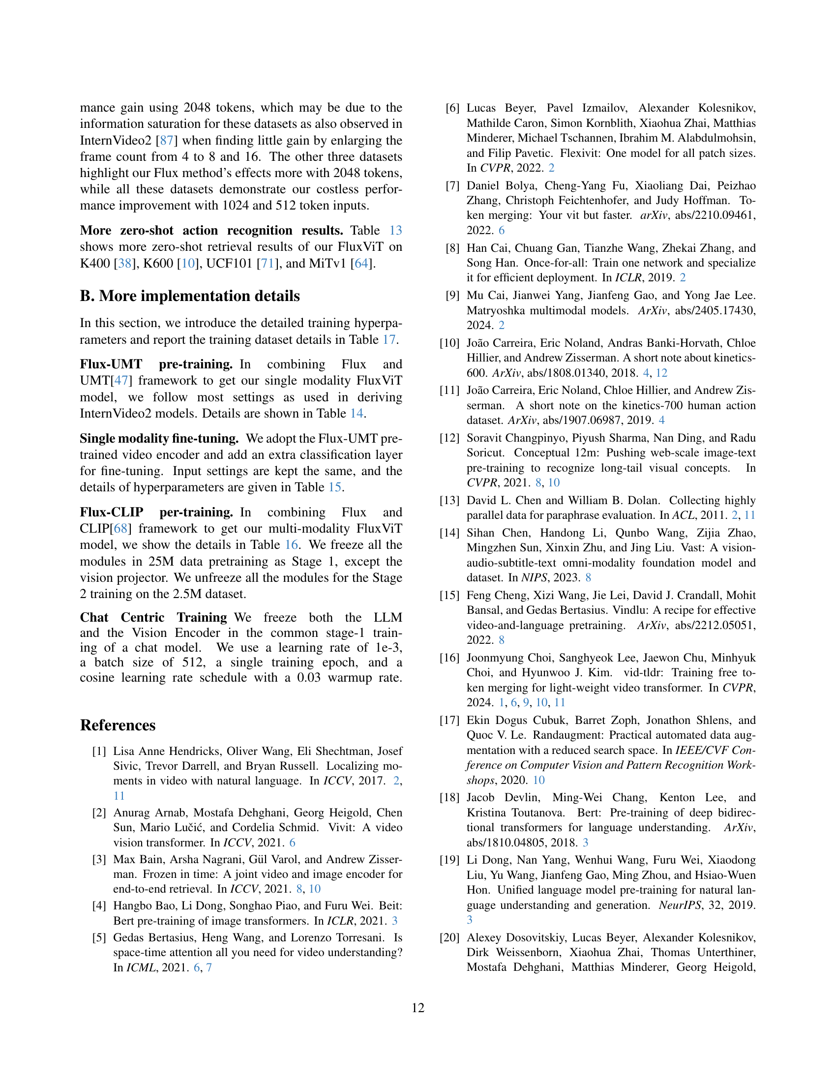
🔼 This table presents zero-shot text-to-video retrieval results on five benchmark datasets: MSRVTT, DiDeMo, ActivityNet, LSMDC, and MSVD. The metric used is R@1 (recall at 1), measuring the accuracy of retrieving the correct video given a text query. The table is structured to compare different variants of the FluxViT model with varying input token numbers (2048, 1024, 512), which correspond to different spatiotemporal resolutions of the input video. For each token count, results are shown for the model using standard training (without masking) and the model using the Flux method’s more informative token selection strategy. The ‘Type’ column indicates whether the task is text-to-video (T2V) or video-to-text (V2T), The dual softmax loss function is employed in all evaluations.
read the caption
Table 9: Zero-shot text-to-video retrieval on MSRVTT (“MSR”), DiDeMo (“DDM”), AcitivityNet (“ANet”), LSMDC, and MSVD. We only report the R@1 accuracy. The upper line regarding FluxViT shows results with non-masked 8×\times×2242, 4×\times×2242 and 2×\times×2242 input setting as indicated by the token count while each lower bold line shows results further using more informative tokens. We employ Dual Softmax Loss for the results.
| Encoder | #Tokens | w/ TO | MVbench | Dream1k-F1 |
| Clip-L [68] | 8256 | ✗ | 45.6 | 28.4 |
| SigLIP336-L [96] | 8576 | ✗ | 46.7 | 29.2 |
| InternVideo2-L [87] | 8224 | ✗ | 47.0 | 28.7 |
| SigLIP336-L [96] | 4576 | ✗ | 44.5 | 25.4 |
| UMT-L [47] | 4256 | ✗ | 45.0 | 24.6 |
| 8256 | 48.3 | 29.0 | ||
| 4256 | 46.9 | 27.9 | ||
| FluxViT-L | 2256 | ✗ | 46.0 | 25.6 |
| 2048 | 49.0 (0.7) | 29.5 (0.5) | ||
| 1024 | 47.7 (0.8) | 28.5 (0.6) | ||
| FluxViT-L | 512 | ✓ | 47.6 (1.6) | 27.5 (1.9) |
🔼 Table 10 presents the performance of various models on two chat-centric benchmark datasets: MVbench (evaluating general perception capabilities) and Dream1k (assessing fine-grained captioning abilities). A key aspect of this experiment is that both the vision encoder (the model being evaluated) and the language model (LLM) remain frozen during training; only a projection layer between them is trained. This setup, referred to as the ’linear prob’ setting, isolates the performance of the vision encoder. The ‘#Tokens’ column indicates the number of visual tokens processed by the vision encoder in each model.
read the caption
Table 10: Results on Chat-Centric benchmarks MVbench (General perception) and Dream1k(Fine-grained caption). Models are trained in a multimodal ‘linear prob’ setting where both the Encoder and the LLM are frozen. #Tokens for the number of visual tokens by the vision encoder.
| #Frame | Spatial Resolution | Max | ||||
| 168 | 196 | 224 | 252 | 280 | ||
| 4 | 80.4 | 81.7 | 82.3 | 82.6 | 82.3 | 82.6 |
| 6 | 83.5 | 84.5 | 84.3 | 84.2 | 83.6 | 84.5 |
| 8 | 84.4 | 84.8 | 84.6 | 84.4 | 83.7 | 84.8 |
| 10 | 85.2 | 85.1 | 85.0 | 84.5 | 83.5 | 85.2 |
| 12 | 85.3 | 85.3 | 84.9 | 84.4 | 83.4 | 85.3 |
| 16 | 85.3 | 85.1 | 84.8 | 84.4 | 83.5 | 85.3 |
| 20 | 85.1 | 85.0 | 84.6 | 84.0 | 83.2 | 85.1 |
| Max | 85.3 | 85.3 | 85.0 | 84.5 | 83.7 | - |
🔼 This table presents the performance of the FluxViT-S model on the K400 dataset. It investigates the impact of varying spatiotemporal resolutions (frame counts and spatial resolutions) while keeping the number of input tokens constant at 1024. The results highlight the optimal balance between frame counts and resolution for achieving the best performance. Each row shows the top-1 accuracy for different settings, with the best accuracy for each frame count shown in bold. The results using the standard, unmasked setting (without the Flux module) are also included in blue for comparison.
read the caption
Table 11: Results of FluxViT-S on K400 using 1024 tokens and different spatiotemporal resolutions. We use 1clip ×\times× 1crop for testing. The blue value marks the results of the unmasked setting. The values in bold show the best resolution for each frame count.
| Method | Input Size | #Token | ||
| 1024 | 512 | |||
| Our selector | 42242 | 82.3 | 79.5 | |
| 82242 | 84.6 | 81.3 | ||
| 122242 | 84.9 | 80.7 | ||
| 162242 | 84.8 | 80.7 | ||
| 202242 | 84.6 | 80.3 | ||
| 242242 | 84.6 | 80.3 | ||
| Max | 84.9 | 81.3 | ||
| w/ Vid-TLDR | 42242 | 77.4 | 78.2 | |
| 82242 | 83.9 | 81.0 | 79.8 | |
| 122242 | 85.0 | 81.4 | 80.6 | |
| 162242 | 85.3 | 81.5 | 80.9 | |
| 202242 | 85.2 | 80.9 | 80.4 | |
| 242242 | 85.2 | 80.5 | 80.3 | |
| Max | 85.3 | 81.5 | 80.9 | |
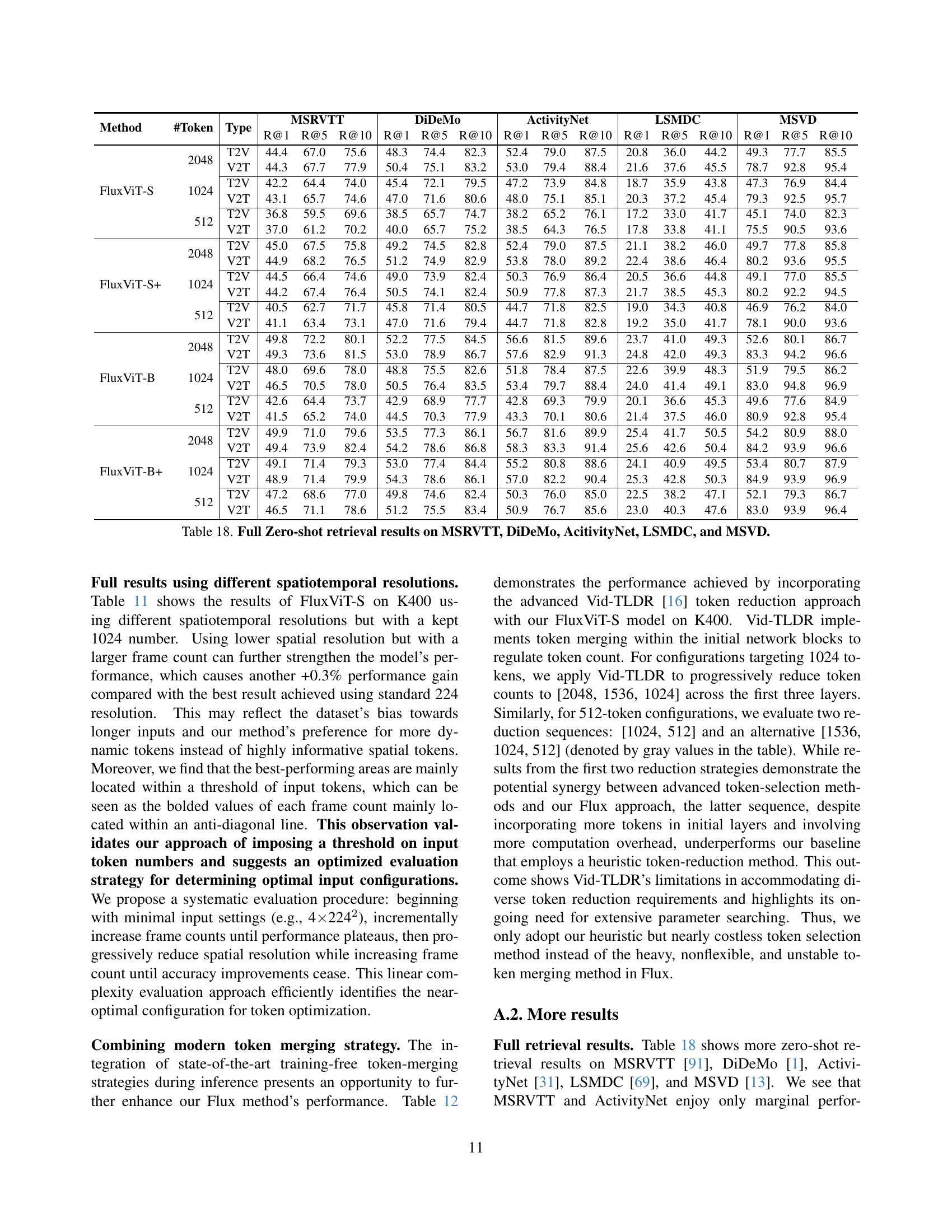
🔼 Table 12 presents an ablation study on the impact of integrating the Vid-TLDR token merging technique [16] within the FluxViT model, specifically during testing on the K400 dataset. The primary goal is to evaluate the effect of different token reduction strategies on the model’s performance. The table compares the top-1 accuracy of FluxViT with varying input spatial and temporal resolutions (indicated by the number of tokens). It showcases that the performance gains obtained by using Vid-TLDR are significantly influenced by the specific hyperparameters employed (particularly the number of tokens reduced in specific layers of the network). This highlights the sensitivity and complexity of adjusting the Vid-TLDR technique for optimal performance.
read the caption
Table 12: Use token merging strategy Vid-TLDR [16] on FluxViT K400 testing. The increment achieved by ViD-TLDR is sensitive to the hyper-parameter setting, like how many tokens are to be reduced in certain layers.
| config | SthSth V2 | Others |
| optimizer | AdamW [58] | |
| optimizer momentum | ||
| weight decay | 0.05 | |
| learning rate schedule | cosine decay [59] | |
| learning rate | 1e-3 | |
| batch size | 2048 | |
| warmup epochs [25] | 20 | |
| total epochs | 100 | |
| teacher input token | 2048 | |
| student input tokens | 2048, 1536, 1024 | |
| input frame | (4, 26, stride=2) | |
| spatial resolution | (168, 280, stride=28) | |
| drop path [34] | 0.05 | |
| flip augmentation | no | yes |
| augmentation | MultiScaleCrop [0.66, 0.75, 0.875, 1] | |
🔼 This table presents the results of zero-shot action recognition experiments. It shows the performance of the FluxViT model, with various configurations (different numbers of input tokens and whether or not advanced Flux modules were used), on several standard action recognition datasets (UCF101 and MiTv1). The results are displayed as Top-1 and Top-5 accuracy rates, providing a comprehensive comparison of the model’s performance across different settings.
read the caption
Table 13: Full Zero-shot Action Recognition Results.
| config | Kinetics | COIN |
| optimizer | AdamW [58] | |
| optimizer momentum | ||
| weight decay | 0.05 | |
| learning rate schedule | cosine decay [59] | |
| learning rate | 2e-4 | 5e-4 |
| batch size | 1024+512 | 512 |
| warmup epochs [25] | 5+1 | 5 |
| total epochs | 35+5 (S), 20+3 (B) | 40(S), 25 (B) |
| drop path [34] | 0.1 | |
| flip augmentation | yes | |
| label smoothing [73] | 0.0 | |
| augmentation | RandAug(9, 0.5) [17] | |
🔼 This table details the hyperparameters used for pre-training the video models using the Unmasked Teacher (UMT) framework with the proposed Flux method. It includes settings for the optimizer, weight decay, learning rate schedule and its initial value, batch size, warm-up epochs, total training epochs, dropout rate, data augmentation techniques, and other relevant parameters. These settings are crucial for achieving robust and efficient pre-training of the video models, especially when using the flexible sampling strategy introduced by the Flux method.
read the caption
Table 14: Flux-UMT pre-training settings.
| config | 25M+2.5M |
| optimizer | AdamW [58] |
| optimizer momentum | |
| weight decay | 0.02 |
| learning rate schedule | cosine decay [59] |
| learning rate | 4e-4 (25M), 2e-5 (2.5M) |
| batch size | 4096 (image), 4096 (video) |
| warmup epochs [25] | 0.6 (25M), 0 (2.5M) |
| total epochs | 3 (25M), 1 (2.5M) |
| input frame | (4, 26, stride=2) |
| spatial resolution | (168, 280, stride=28) |
| token threshold | (2048, 4096) |
| augmentation | MultiScaleCrop [0.5, 1] |
🔼 Table 15 details the hyperparameters used for fine-tuning the model on the action recognition task. Specifically, it shows the optimizer used (AdamW), optimizer momentum, weight decay, learning rate schedule (cosine decay), learning rate, batch size, warmup epochs, total training epochs, dropout rate, data augmentation techniques used (flip augmentation and RandAugment), and label smoothing. The training epochs are broken down into two phases: A epochs on the Kinetics-710 dataset and B epochs on the Kinetics-400 dataset. Warmup epochs and batch sizes follow the same A/B breakdown.
read the caption
Table 15: Action recognition fine-tuning settings. The training epochs A+B on Kinetics include A epochs on K710 and B epochs on K400, the same notation for warmup-epochs and batch size.
| Dataset | #image/video | #text | Type |
| Kinetics-710 [44] | 658K | 0 | Video |
| COCO [52] | 113K | 567K | image |
| Visual Genome [39] | 100K | 768K | image |
| SBU Captions [65] | 860K | 860K | image |
| CC3M [70] | 2.88M | 2.88M | image |
| CC12M [12] | 11.00M | 11.00M | image |
| S-MiT0.5M [63] | 0.5M | 0.5M | video |
| WebVid-2M [3] | 2.49M | 2.49M | video |
| WebVid-10M [3] | 10.73M | 10.73M | video |
| InternVid2M [86] | 2.0M | 2.0M | video |
| 25M corpus = CC3MCC12M | 25.68M | 26.81M | video + image |
| WebVid-10MVisual Genome | |||
| SBUCOCO | |||
| 2.5M corpus = S-MiTInternVid2MCOCO | 2.56M | 2.62M | video + image |
🔼 This table details the hyperparameters used during the pre-training phase of the Flux-CLIP model. It outlines the optimizer used (AdamW), its momentum, weight decay, learning rate schedule, learning rate itself, batch size, warmup epochs, total training epochs, dropout rate, data augmentation techniques (flip augmentation and MultiScaleCrop), and the specific handling of batch size for the FluxViT-B model during training with the 2.5M dataset. The note clarifies that the batch size was reduced to 2048 for FluxViT-B model when training with the 2.5M dataset.
read the caption
Table 16: Flux-CLIP pre-training settings. ††{\dagger}†: For FluxViT-B, we lower the batch size to 2048 for the 2.5M data training.
Full paper#