TL;DR#
Generating realistic world simulations is challenging, especially bridging the gap between synthetic and real environments. Existing methods often lack precise control over different aspects of the generated world, hindering their use in applications like robotics & autonomous driving.
To tackle these issues, this paper introduces a novel conditional world generation model. It uses multiple spatial control inputs (segmentation, depth, edge) and applies adaptive weighting. This enables precise control and is customizable. The model is highly controllable and finds use in world-to-world transfers and can achieve real-time world generation through an inference scaling strategy.
Key Takeaways#
Why does it matter?#
This research on adaptable world generation is significant, offering potential for various applications like Sim2Real and robotics. By allowing weighted control over diverse modalities, it paves the way for creating more realistic and controllable simulations. The study’s real-time generation achievement and open-source availability can accelerate developments in the field.
Visual Insights#
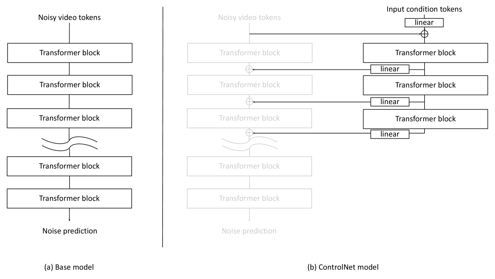
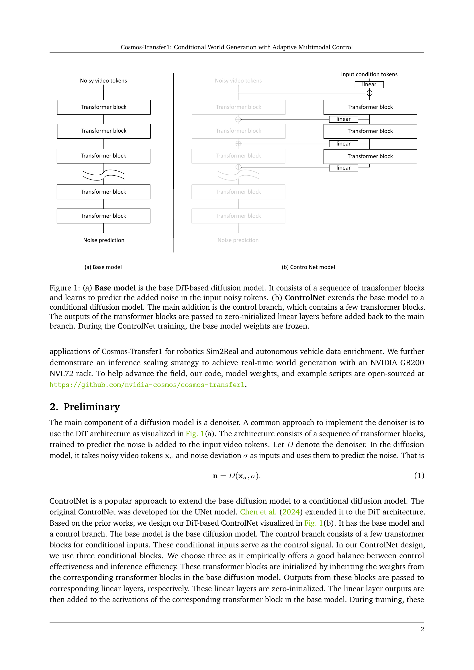
🔼 Figure 1 illustrates the architecture of the Cosmos-Transfer1 model. Panel (a) shows the base diffusion model, which is a sequence of transformer blocks that predict the noise added to the input video tokens during the diffusion process. Panel (b) shows the ControlNet model, which is an extension of the base model. It adds a control branch consisting of several transformer blocks. The output of each control block is fed into a zero-initialized linear layer and then added to the corresponding block in the main branch. The weights of the base model are frozen during the training of the ControlNet.
read the caption
Figure 1: (a) Base model is the base DiT-based diffusion model. It consists of a sequence of transformer blocks and learns to predict the added noise in the input noisy tokens. (b) ControlNet extends the base model to a conditional diffusion model. The main addition is the control branch, which contains a few transformer blocks. The outputs of the transformer blocks are passed to zero-initialized linear layers before added back to the main branch. During the ControlNet training, the base model weights are frozen.
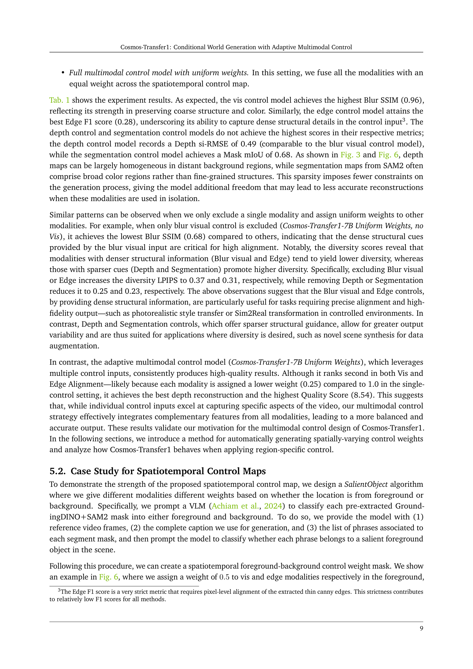
| Model | Vis Alignment | Edge Alignment | Depth Alignment | Segmentation Alignment | Diversity | Overall Quality |
| Blur SSIM | Edge F1 | Depth si-RMSE | Mask mIoU | Diversity LPIPS | Quality Score | |
| Cosmos-Transfer1-7B [Vis] | 0.96 | 0.16 | 0.49 | 0.72 | 0.19 | 5.94 |
| Cosmos-Transfer1-7B [Edge] | 0.77 | 0.28 | 0.53 | 0.71 | 0.28 | 5.48 |
| Cosmos-Transfer1-7B [Depth] | 0.71 | 0.14 | 0.49 | 0.70 | 0.39 | 6.51 |
| Cosmos-Transfer1-7B [Seg] | 0.66 | 0.11 | 0.75 | 0.68 | 0.42 | 6.30 |
| Cosmos-Transfer1-7B Uniform Weights, no Vis | 0.68 | 0.13 | 0.57 | 0.67 | 0.37 | 8.02 |
| Cosmos-Transfer1-7B Uniform Weights, no Edge | 0.81 | 0.10 | 0.53 | 0.66 | 0.31 | 7.68 |
| Cosmos-Transfer1-7B Uniform Weights, no Depth | 0.83 | 0.15 | 0.52 | 0.69 | 0.25 | 7.49 |
| Cosmos-Transfer1-7B Uniform Weights, no Seg | 0.84 | 0.15 | 0.43 | 0.70 | 0.23 | 7.83 |
| Cosmos-Transfer1-7B Uniform Weights | 0.87 | 0.20 | 0.47 | 0.72 | 0.22 | 8.54 |
🔼 This table presents a quantitative comparison of different Cosmos-Transfer1 model configurations on the TransferBench dataset. It contrasts the performance of models using only a single control modality (e.g., visual, edge, depth, segmentation) against those utilizing multiple modalities with uniform weighting. The ‘Cosmos-Transfer1-7B, Uniform Weights’ row represents the model employing all four modalities equally (each weighted at 0.25). Other multimodal rows show results when one modality is excluded. The table evaluates each configuration using metrics such as Blur SSIM, Edge F1, Depth si-RMSE, Mask mIoU, Diversity LPIPS, and an overall Quality Score. Best performing results for each metric are highlighted in bold, while second-best results are underlined.
read the caption
Table 1: Quantitative evaluation on TransferBench for various Cosmos-Transfer1 configurations. We compare single control models (each conditioned on a single modality) with multimodal variants that use spatially uniform weights. For the multimodal cases, “Cosmos-Transfer1-7B, Uniform Weights” denotes the full model that integrates all four control modalities (each weighted at 0.25), while variants such as “Cosmos-Transfer1-7B, Uniform Weights, No Vis” exclude a specific modality (here, the blur visual control), with the remaining modalities retaining equal weights. Best results are in bold; second-best are underlined.
In-depth insights#
Adaptive Control#
Adaptive control dynamically adjusts a system’s parameters to maintain optimal performance amidst changing conditions or uncertainties. It contrasts with fixed control strategies, offering greater robustness. Key methods include model reference adaptive control (MRAC), which aims to match the system’s behavior to a desired reference model, and self-tuning regulators (STR), where the controller parameters are estimated and updated online. Adaptive control is crucial in applications with significant parameter variations, such as aerospace, robotics, and process control. Challenges involve ensuring stability and convergence of the adaptive algorithms, as well as dealing with disturbances and unmodeled dynamics. Recent advances focus on robust adaptive control techniques, incorporating learning-based methods to improve adaptability and performance in complex environments. The goal is to create systems that learn and adjust automatically.
Multimodal Fusion#
While “Multimodal Fusion” isn’t explicitly discussed as a heading, the paper heavily implies its importance through the introduced “Cosmos-Transfer1” model. The paper leverages multiple modalities like segmentation, depth, and edge to generate world simulations, hinting at an inherent fusion process. Effective fusion would mean the model intelligently combines information from various sources. Adaptive weighting, a key feature, suggests a sophisticated fusion strategy where the influence of each modality varies spatially and temporally. The model has an ability to learn to prioritize depth cues for geometry preservation or edge information for fine-grained details. The success of the model indicates the importance of the multimodal fusion, specifically the interplay between different signals and the benefit on control and overall generation quality. A study on how well the modalities aligns with each other is very crucial, especially with the diversity of modalities (depth, segmentation), it needs to be aligned in a way that ensures the model can leverage each modality. An appropriate loss function or metric to measure the alignment between these modalities is very beneficial for training.
Sim2Real Bridge#
Sim2Real emerges as a pivotal theme, addressing the challenge of transferring models trained in simulated environments to real-world applications. The research recognizes the domain gap between synthetic and real data, necessitating innovative methods. Generative AI models are explored to bridge this gap by refining simulator outputs, enhancing realism, and preserving task-relevant properties. The paper introduces a diffusion-based conditional world model with adaptive weighting scheme, enabling highly controllable world generation and improved generation quality. By leveraging modalities, the model effectively preserves scene structure and addresses visual fidelity. The approach leverages NVIDIA Omniverse with physically-based sensor simulation and is effective to enhance the visual diversity of simulated scenes. It offers a promising avenue for improving the robustness and generalization of models trained in simulation for real-world robotic and autonomous driving tasks. With the adaptive weighting scheme, Cosmos-Transfer1 ensures key elements in the simulation are retained when transferring the simulation to the real world.
Real-Time Gen.#
Given the limited context of just the phrase “Real-Time Gen,”, one can infer that the research paper likely addresses the challenge of achieving real-time or near real-time generation of content, potentially in the context of video or image synthesis. This implies a focus on optimizing the generation process to minimize latency, which is crucial for interactive applications or scenarios requiring immediate feedback. The paper might delve into specific architectural choices, such as model compression techniques or specialized hardware acceleration (e.g., using GPUs or specialized ASICs), to achieve the desired performance. Data parallelism and model parallelism are potentially used for scaling up the generation process. The success of real-time generation is heavily influenced by the trade-off between generation speed and quality, requiring careful consideration of algorithmic complexity and resource allocation. The research could also explore novel methods for accelerating the generation process, such as exploiting sparsity in the model or employing approximate computation techniques.
AI+Physical World#
AI’s intersection with the physical world marks a transformative shift, enabling digital systems to interact with and understand real-world environments. This convergence fuels advancements in robotics, autonomous vehicles, and augmented reality, blurring the lines between virtual and physical domains. Generative AI models, particularly those conditioned on multimodal inputs like images, depth maps, and semantic segmentations, are instrumental in bridging this gap, allowing for the creation of realistic simulations and enabling AI agents to learn and operate effectively in complex physical settings. Challenges include ensuring robustness to noisy sensor data, maintaining physical plausibility in generated content, and addressing safety concerns in real-world deployments. Future directions involve exploring novel sensor modalities, developing more efficient and interpretable models, and establishing robust evaluation metrics for AI systems operating in the physical world.
More visual insights#
More on figures
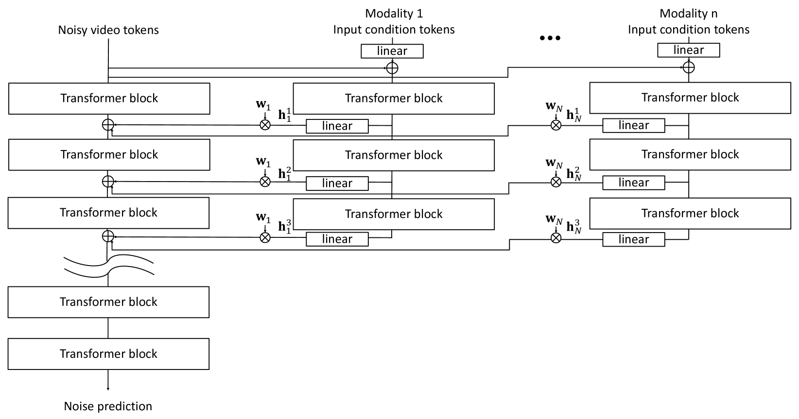
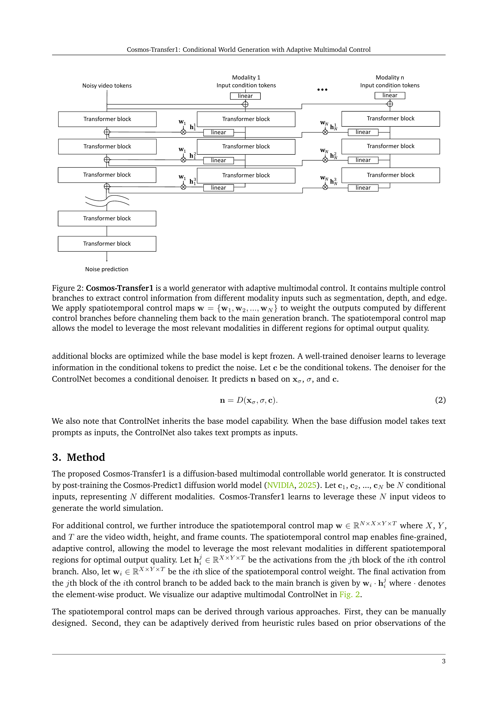
🔼 Cosmos-Transfer1 uses multiple control branches to process different input modalities (segmentation, depth, and edge). A spatiotemporal control map assigns weights to each modality’s output at each spatial location and time step, allowing the model to emphasize certain modalities in specific areas. This adaptive weighting scheme enables fine-grained control over world generation, maximizing output quality by using the most relevant information for each region. The weighted outputs of the control branches are combined and fed into the main generation branch.
read the caption
Figure 2: Cosmos-Transfer1 is a world generator with adaptive multimodal control. It contains multiple control branches to extract control information from different modality inputs such as segmentation, depth, and edge. We apply spatiotemporal control maps 𝐰={𝐰1,𝐰2,…,𝐰N}𝐰subscript𝐰1subscript𝐰2…subscript𝐰𝑁\mathbf{w}=\{\mathbf{w}_{1},\mathbf{w}_{2},...,\mathbf{w}_{N}\}bold_w = { bold_w start_POSTSUBSCRIPT 1 end_POSTSUBSCRIPT , bold_w start_POSTSUBSCRIPT 2 end_POSTSUBSCRIPT , … , bold_w start_POSTSUBSCRIPT italic_N end_POSTSUBSCRIPT } to weight the outputs computed by different control branches before channeling them back to the main generation branch. The spatiotemporal control map allows the model to leverage the most relevant modalities in different regions for optimal output quality.
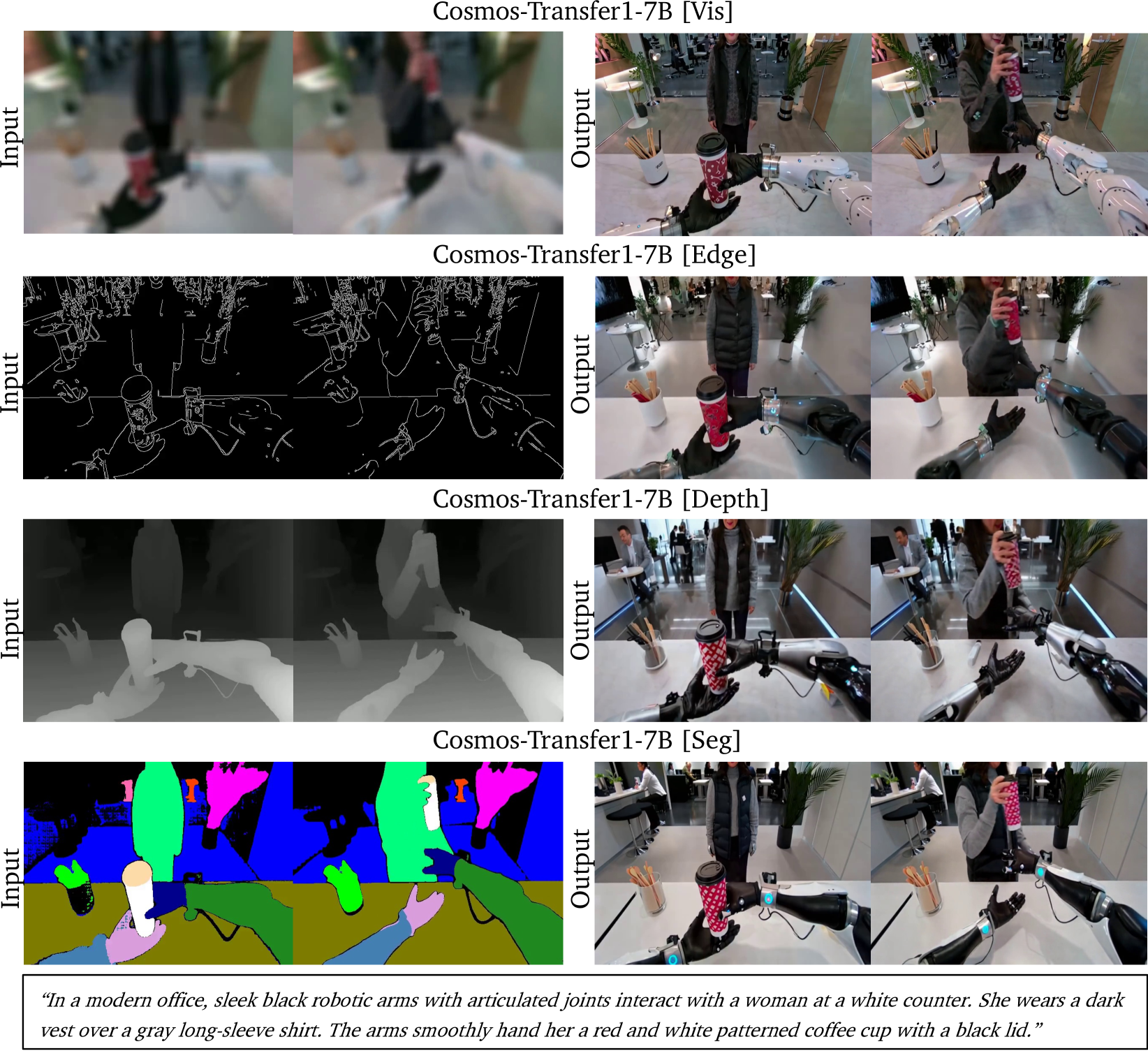
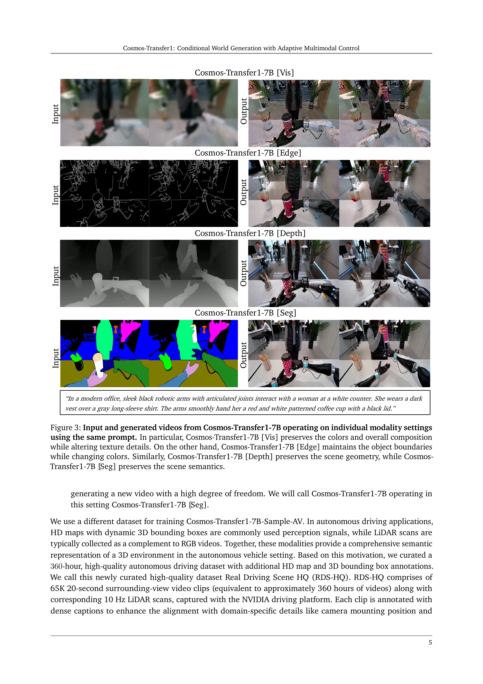
🔼 This figure shows the input and output videos generated by the Cosmos-Transfer1-7B model under various settings. The model was given the same text prompt for each condition. The four conditions tested show how each individual modality (visual, edge, depth, and segmentation) affects the final output. Cosmos-Transfer1-7B [Vis] primarily preserves the overall colors and composition of the input video, while modifying texture and detail. Cosmos-Transfer1-7B [Edge] maintains the main object boundaries, but modifies colors and textures more significantly. Cosmos-Transfer1-7B [Depth] focuses on maintaining the overall 3D structure and geometry of the scene, allowing other aspects to vary more freely. Finally, Cosmos-Transfer1-7B [Seg] prioritizes the preservation of semantic information, preserving scene structure and main object categories, and allowing other aspects to vary more freely.
read the caption
Figure 3: Input and generated videos from Cosmos-Transfer1-7B operating on individual modality settings using the same prompt. In particular, Cosmos-Transfer1-7B [Vis] preserves the colors and overall composition while altering texture details. On the other hand, Cosmos-Transfer1-7B [Edge] maintains the object boundaries while changing colors. Similarly, Cosmos-Transfer1-7B [Depth] preserves the scene geometry, while Cosmos-Transfer1-7B [Seg] preserves the scene semantics.
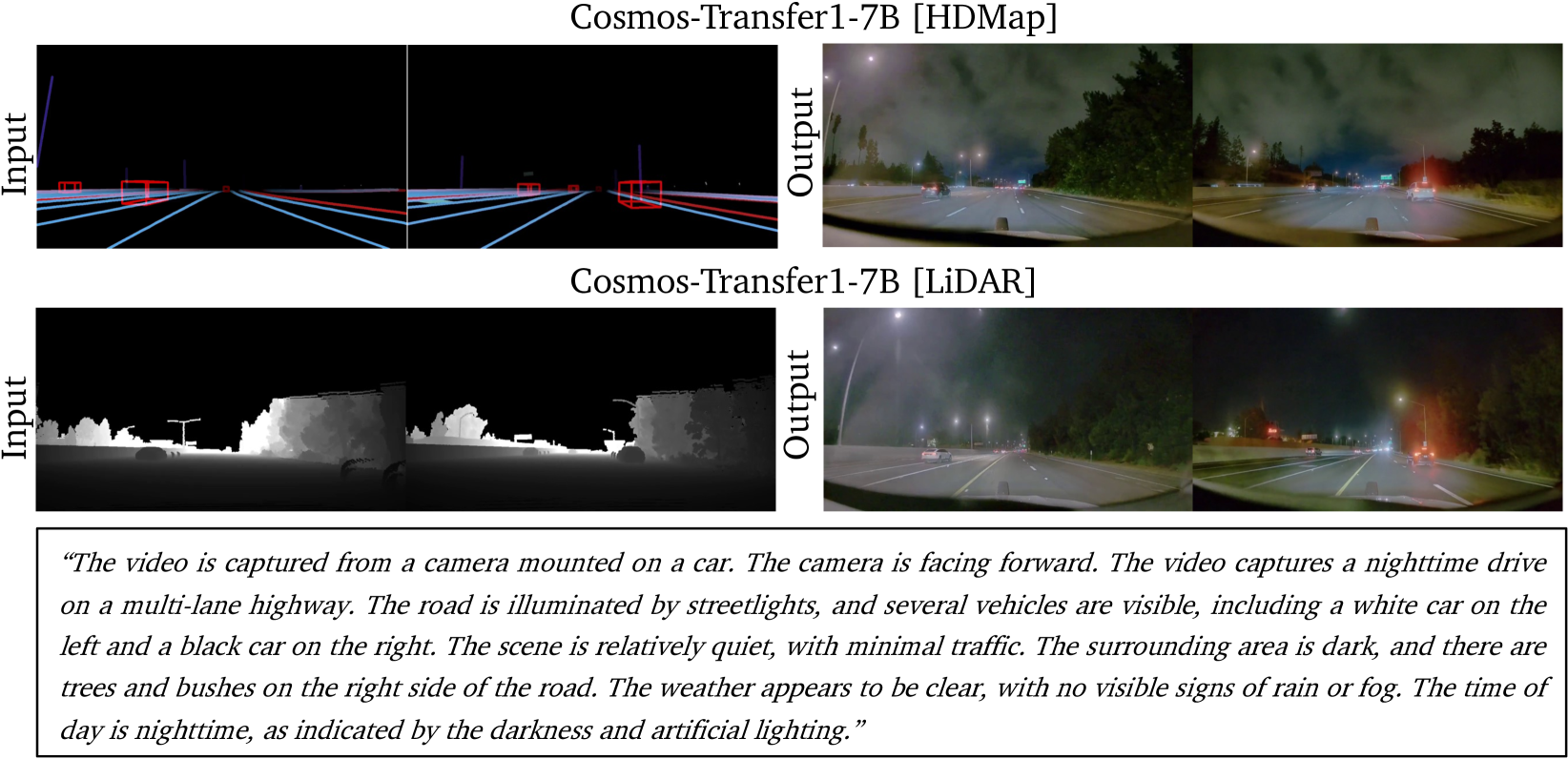
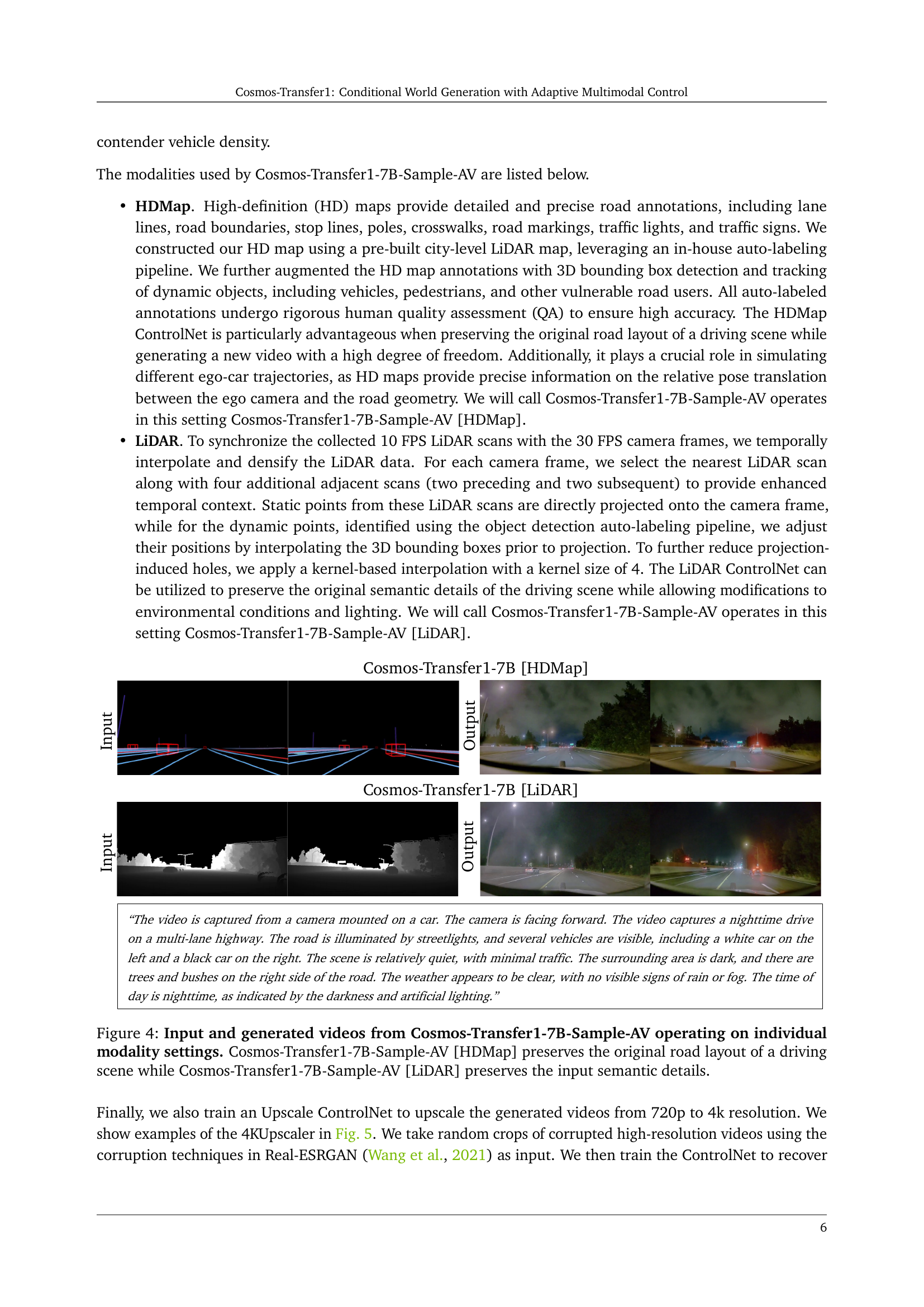
🔼 Figure 4 presents a comparison of input and output videos generated using two different versions of the Cosmos-Transfer1-7B-Sample-AV model, each conditioned on a single modality: HDMap and LiDAR. The left column shows the input videos. The Cosmos-Transfer1-7B-Sample-AV model with HDMap as input successfully preserves the road layout and key structural features of the driving scene. The model with LiDAR as input accurately preserves semantic details like the presence and positioning of vehicles, although some details of the road layout might not be as precise.
read the caption
Figure 4: Input and generated videos from Cosmos-Transfer1-7B-Sample-AV operating on individual modality settings. Cosmos-Transfer1-7B-Sample-AV [HDMap] preserves the original road layout of a driving scene while Cosmos-Transfer1-7B-Sample-AV [LiDAR] preserves the input semantic details.
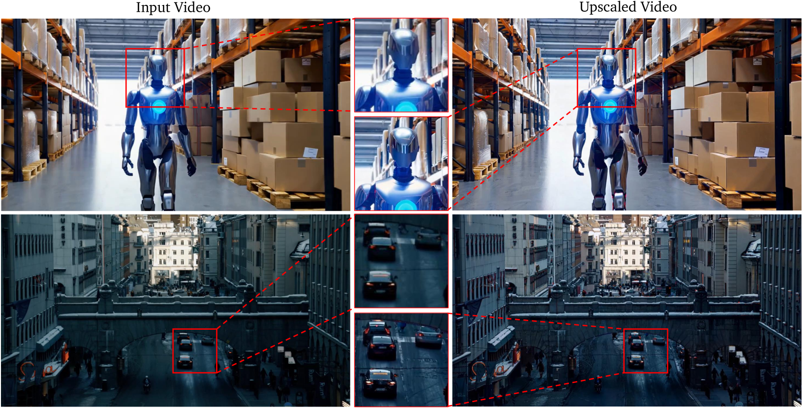
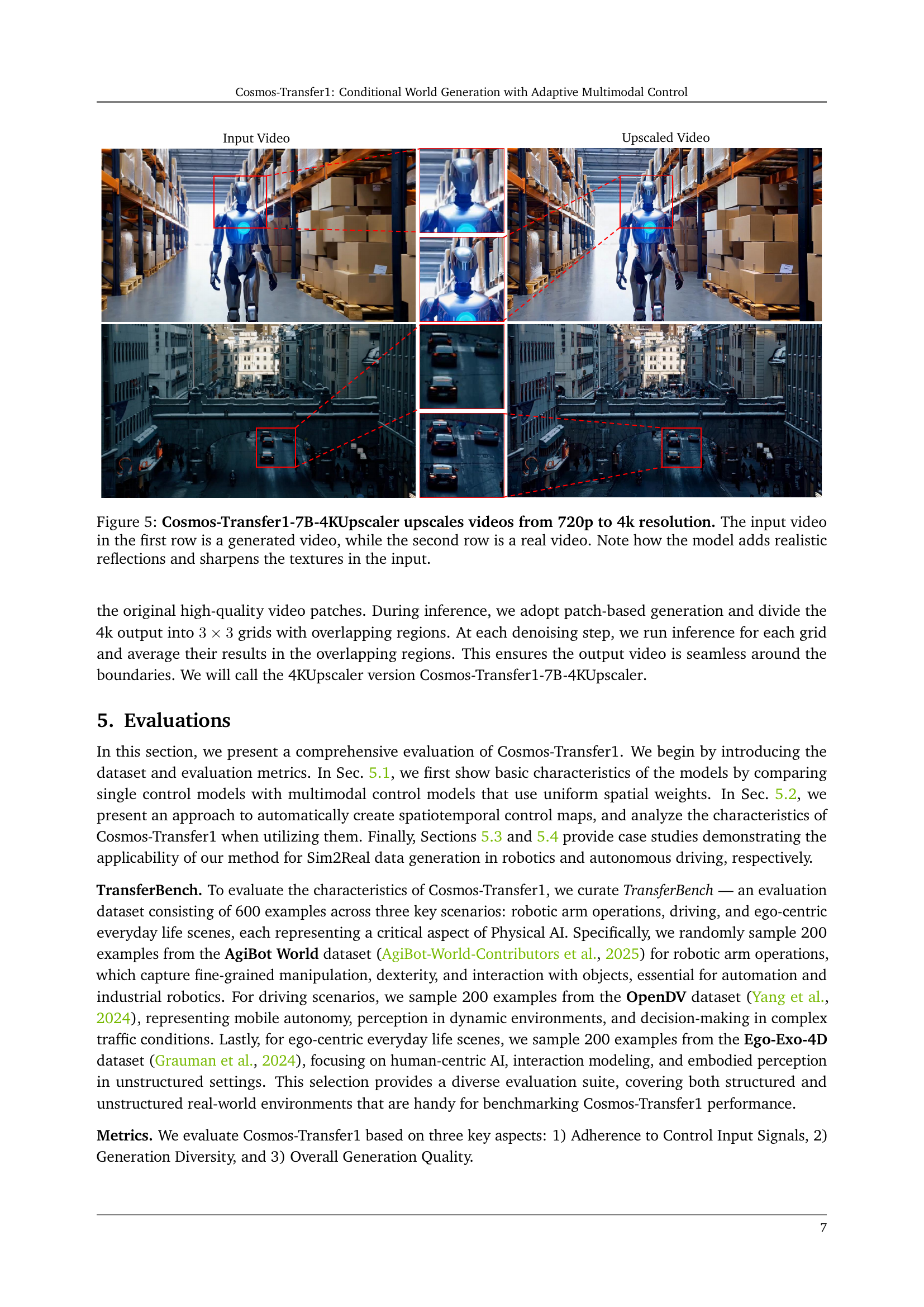
🔼 This figure demonstrates the capability of Cosmos-Transfer1-7B-4KUpscaler to enhance video resolution. The model takes a 720p input video (generated by the model in the top row, and a real video in the bottom row) and upscales it to 4K resolution. The upscaling process not only increases the resolution but also improves the visual quality by adding realistic reflections and sharpening textures, making the generated 4k video more realistic and detailed.
read the caption
Figure 5: Cosmos-Transfer1-7B-4KUpscaler upscales videos from 720p to 4k resolution. The input video in the first row is a generated video, while the second row is a real video. Note how the model adds realistic reflections and sharpens the textures in the input.
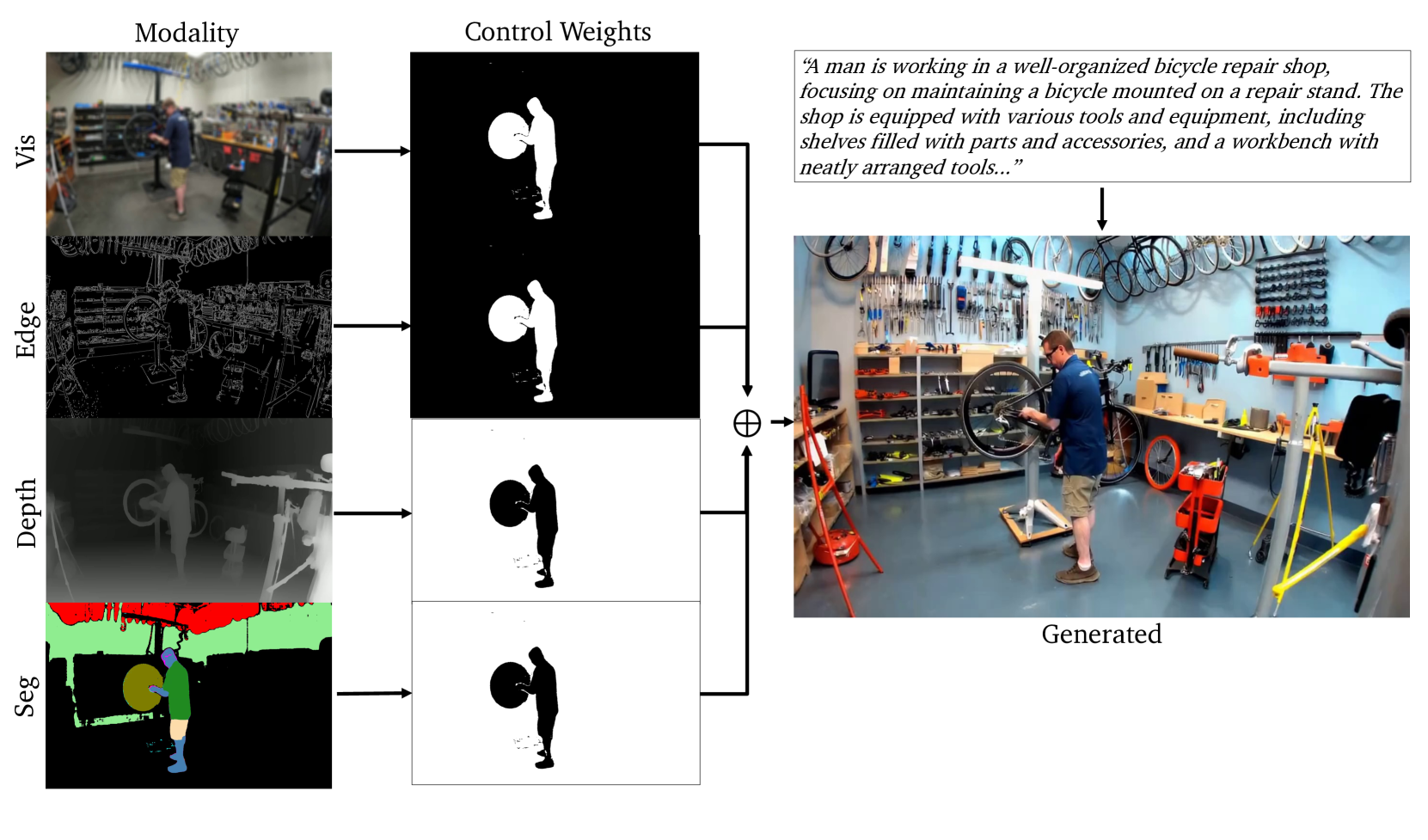
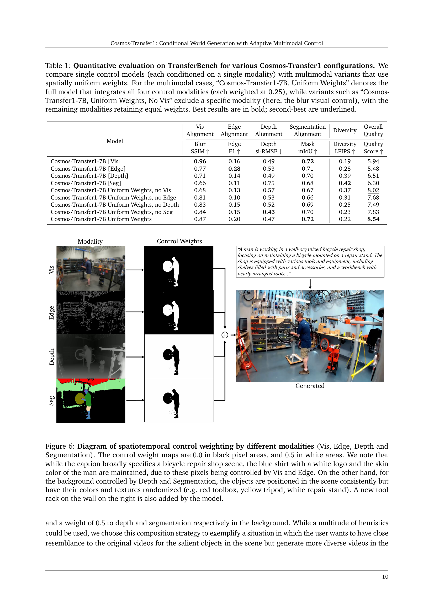
🔼 Figure 6 illustrates the concept of adaptive multimodal control in Cosmos-Transfer1. The image shows spatiotemporal control weight maps applied to different modalities (visual, edge, depth, and segmentation). Black pixels represent a weight of 0, meaning no influence from that modality, while white pixels have a weight of 0.5, indicating moderate influence. The example focuses on a scene described as a bicycle repair shop. The foreground, controlled primarily by visual and edge information, retains details like the man’s blue shirt and skin tone. The background, controlled by depth and segmentation, shows objects in consistent positions but with randomized colors and textures (e.g., a red toolbox instead of a realistic one). Notably, the model even adds a new tool rack to the background, demonstrating its ability to generate novel elements.
read the caption
Figure 6: Diagram of spatiotemporal control weighting by different modalities (Vis, Edge, Depth and Segmentation). The control weight maps are 0.00.00.00.0 in black pixel areas, and 0.50.50.50.5 in white areas. We note that while the caption broadly specifies a bicycle repair shop scene, the blue shirt with a white logo and the skin color of the man are maintained, due to these pixels being controlled by Vis and Edge. On the other hand, for the background controlled by Depth and Segmentation, the objects are positioned in the scene consistently but have their colors and textures randomized (e.g. red toolbox, yellow tripod, white repair stand). A new tool rack on the wall on the right is also added by the model.
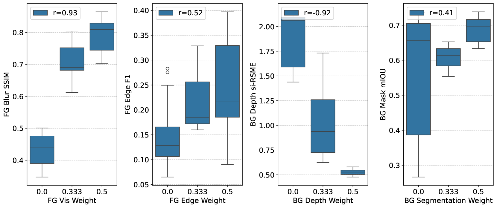
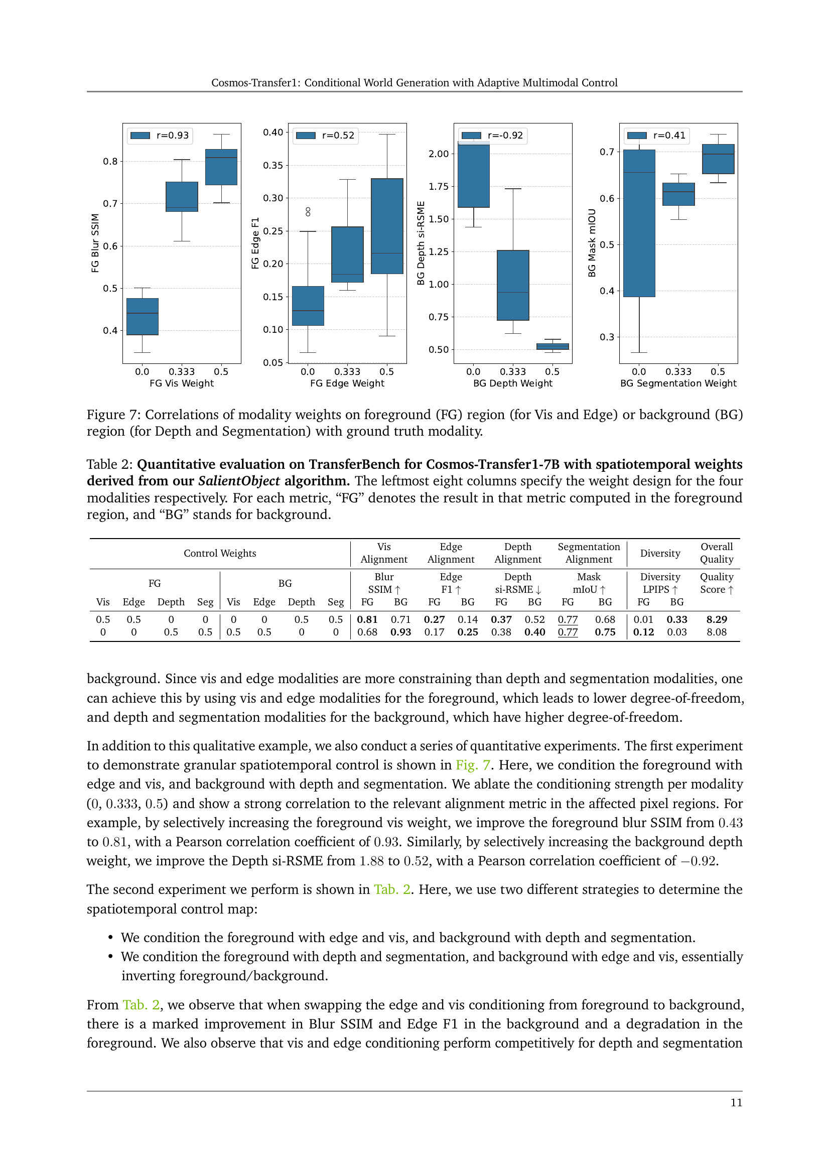
🔼 Figure 7 displays the correlation analysis between the control weights assigned to various modalities (Visual, Edge, Depth, and Segmentation) within the foreground and background regions of generated videos and the corresponding ground truth modalities. Separate graphs illustrate these correlations. The x-axis represents the weight assigned to each modality, while the y-axis shows the alignment score measured by different metrics specific to each modality (e.g., Blur SSIM for Visual). The results reveal the influence of foreground and background weight settings on the final video quality and alignment with control inputs. The positive correlations indicate that increasing the weight of certain modalities, especially in the appropriate regions, improves alignment with the ground truth. This suggests that the model’s ability to adhere to control signals depends significantly on how the control weights are distributed spatially.
read the caption
Figure 7: Correlations of modality weights on foreground (FG) region (for Vis and Edge) or background (BG) region (for Depth and Segmentation) with ground truth modality.

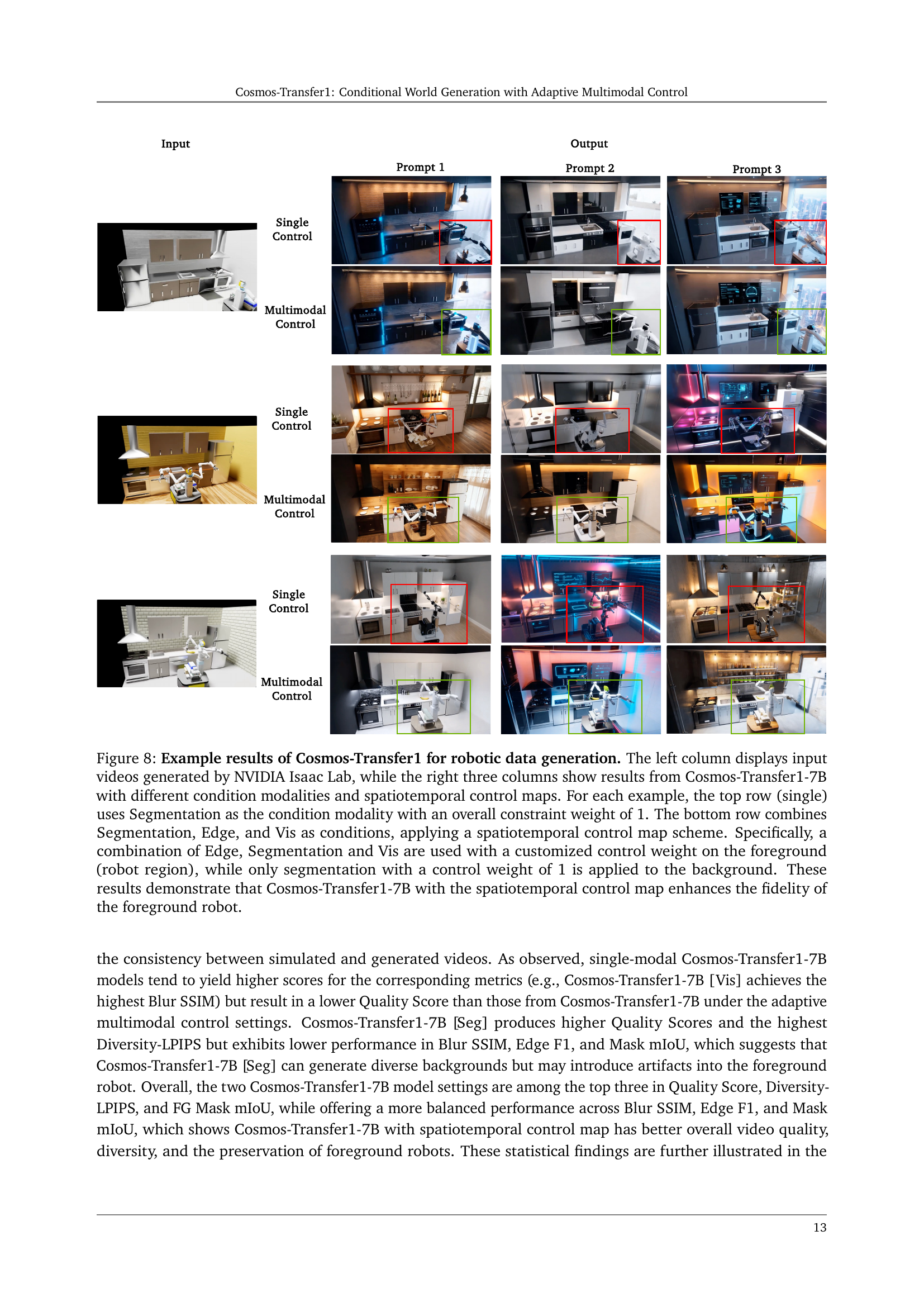
🔼 This figure showcases the results of Cosmos-Transfer1, a model for generating robotic manipulation videos. The leftmost column shows videos from NVIDIA Isaac Lab as input. The remaining columns present outputs from Cosmos-Transfer1-7B under various conditions. Each row represents a single scenario. The top row uses only segmentation as a condition with a weight of 1. The bottom row uses a combination of segmentation, edge, and visual information, employing a spatiotemporal control map that assigns custom weights to the foreground (robot) and background, assigning a weight of 1 only to the background. This comparison highlights how the spatiotemporal control map improves the fidelity of the robot in the foreground by leveraging multiple input modalities.
read the caption
Figure 8: Example results of Cosmos-Transfer1 for robotic data generation. The left column displays input videos generated by NVIDIA Isaac Lab, while the right three columns show results from Cosmos-Transfer1-7B with different condition modalities and spatiotemporal control maps. For each example, the top row (single) uses Segmentation as the condition modality with an overall constraint weight of 1. The bottom row combines Segmentation, Edge, and Vis as conditions, applying a spatiotemporal control map scheme. Specifically, a combination of Edge, Segmentation and Vis are used with a customized control weight on the foreground (robot region), while only segmentation with a control weight of 1 is applied to the background. These results demonstrate that Cosmos-Transfer1-7B with the spatiotemporal control map enhances the fidelity of the foreground robot.

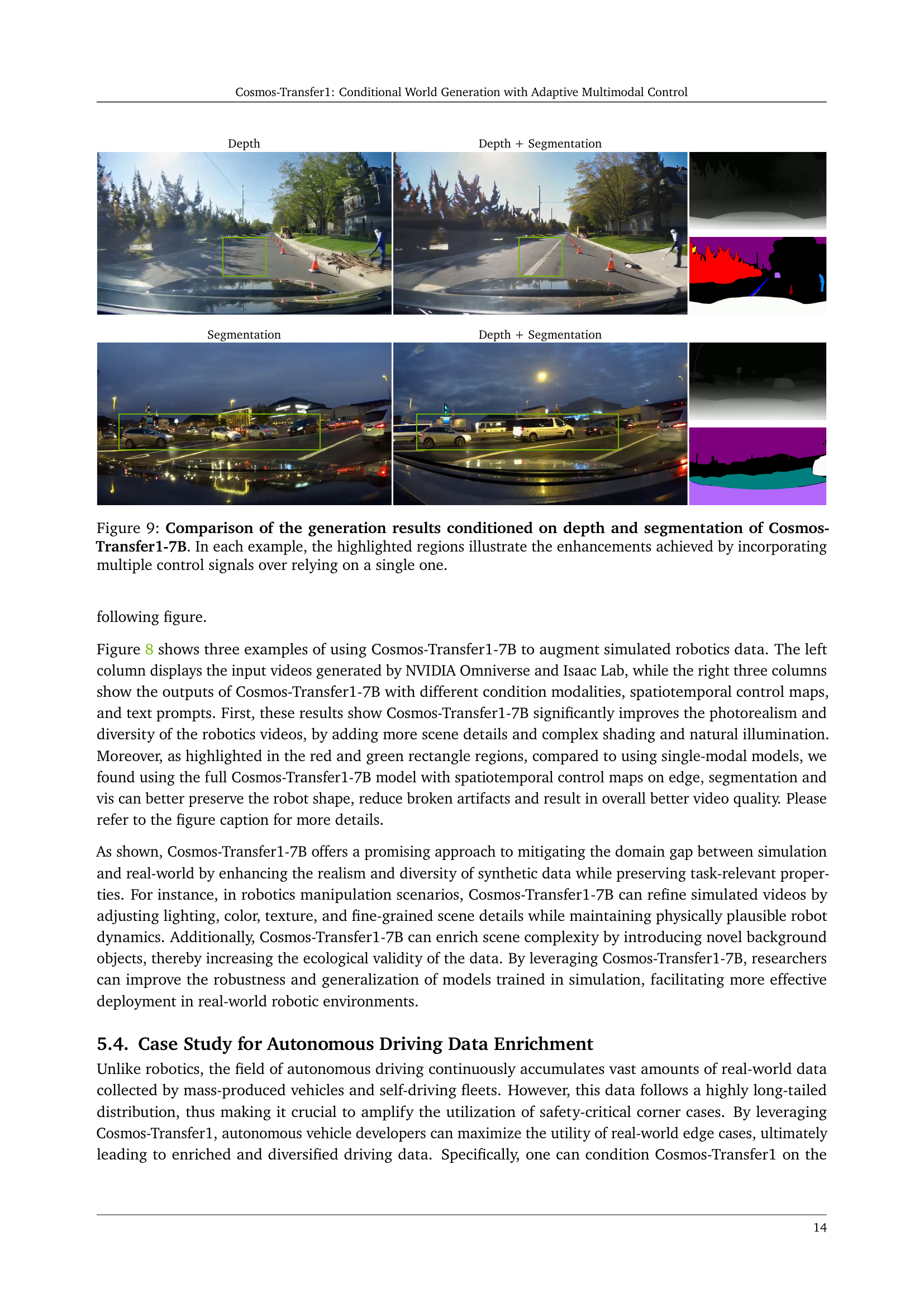
🔼 Figure 9 displays a comparison between the video generation results obtained using Cosmos-Transfer1-7B, a diffusion-based model, with either depth or segmentation as the sole condition and when both are used simultaneously. The highlighted regions in each example showcase the superior generation quality when both depth and segmentation are used as inputs, demonstrating the improvements and additional details that result from incorporating multiple control signals. The figure visually emphasizes the increased realism and accuracy in those regions.
read the caption
Figure 9: Comparison of the generation results conditioned on depth and segmentation of Cosmos-Transfer1-7B. In each example, the highlighted regions illustrate the enhancements achieved by incorporating multiple control signals over relying on a single one.

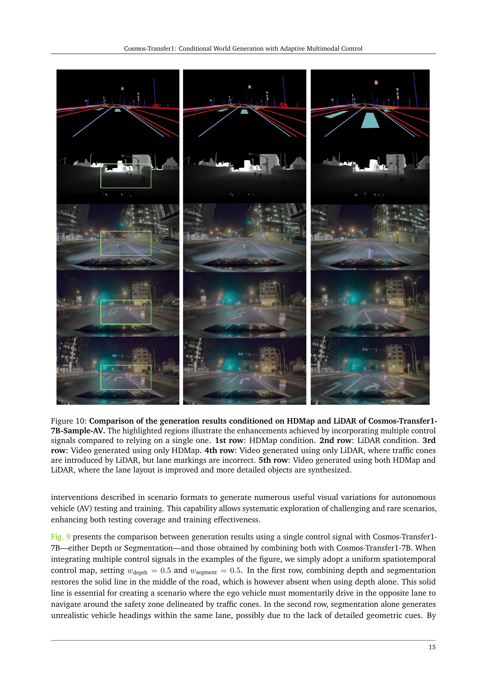
🔼 Figure 10 demonstrates the impact of using both HDMap and LiDAR data as control signals for Cosmos-Transfer1-7B-Sample-AV, a world generation model. The figure shows five rows of images. The first row displays video frames generated using only HDMap data as a control signal. The second row showcases frames generated using only LiDAR data. The third and fourth rows highlight the limitations of using just one data source. The HDMap-only example (row 3) lacks fine details and accurate representations of objects, especially moving vehicles. The LiDAR-only example (row 4) accurately shows traffic cones, but the lane markings are incorrect. The fifth row presents the results when using both HDMap and LiDAR. This combination allows the model to create a more accurate and detailed scene, improving lane markings and object details.
read the caption
Figure 10: Comparison of the generation results conditioned on HDMap and LiDAR of Cosmos-Transfer1-7B-Sample-AV. The highlighted regions illustrate the enhancements achieved by incorporating multiple control signals compared to relying on a single one. 1st row: HDMap condition. 2nd row: LiDAR condition. 3rd row: Video generated using only HDMap. 4th row: Video generated using only LiDAR, where traffic cones are introduced by LiDAR, but lane markings are incorrect. 5th row: Video generated using both HDMap and LiDAR, where the lane layout is improved and more detailed objects are synthesized.

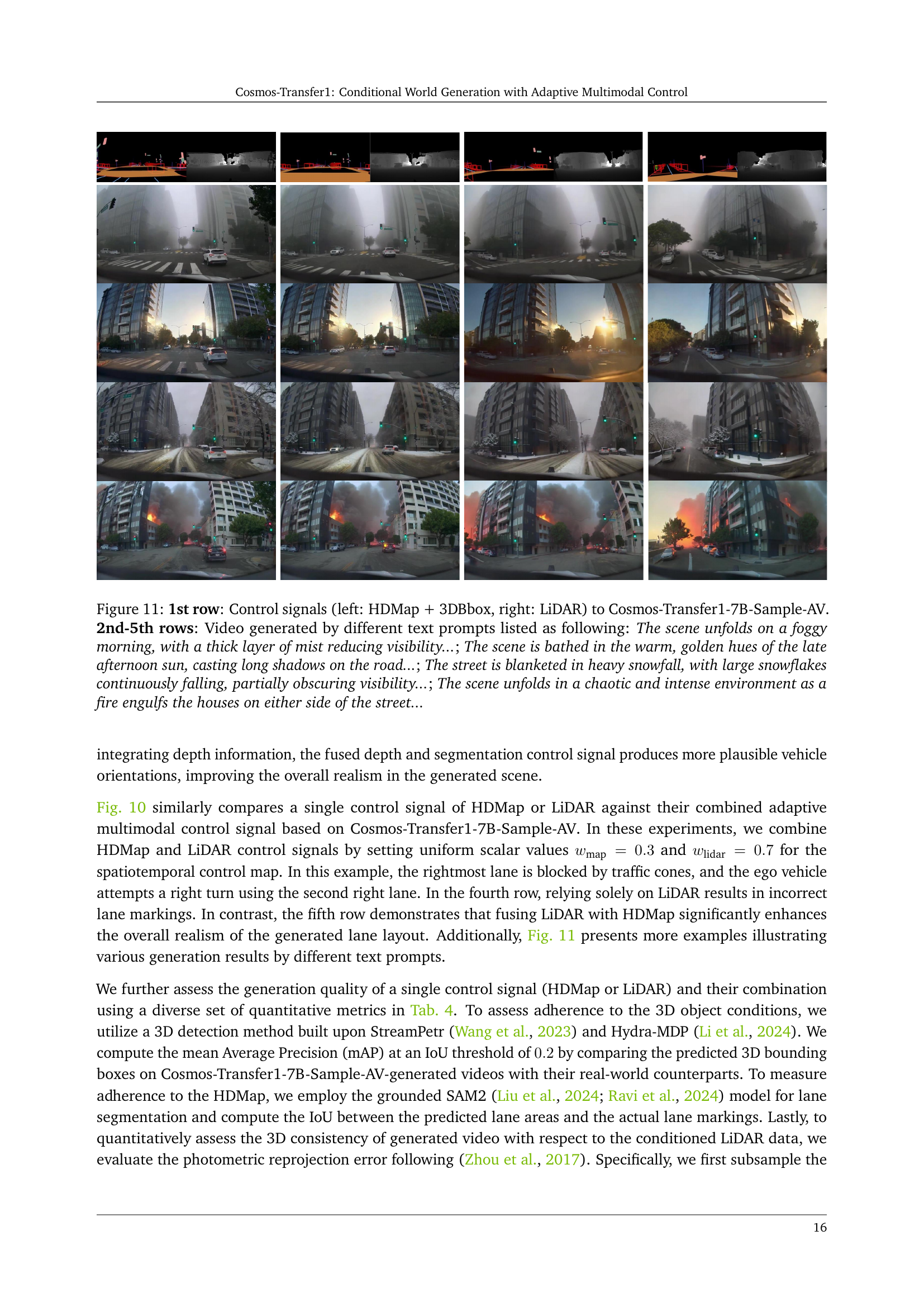
🔼 Figure 11 showcases the capabilities of Cosmos-Transfer1-7B-Sample-AV, a model designed for autonomous driving applications, in generating diverse driving scenarios. The first row displays the input control signals: a high-definition map (HDMap) combined with 3D bounding boxes, and LiDAR data. The subsequent rows (2nd-5th) present videos generated by the model using four different text prompts. These prompts describe varying weather conditions and times of day: a foggy morning, a sunny afternoon, a snowy day, and a scene with a fire. Each generated video demonstrates the model’s ability to create realistic and diverse driving scenes based on both the control signals and the textual descriptions.
read the caption
Figure 11: 1st row: Control signals (left: HDMap + 3DBbox, right: LiDAR) to Cosmos-Transfer1-7B-Sample-AV. 2nd-5th rows: Video generated by different text prompts listed as following: The scene unfolds on a foggy morning, with a thick layer of mist reducing visibility…; The scene is bathed in the warm, golden hues of the late afternoon sun, casting long shadows on the road…; The street is blanketed in heavy snowfall, with large snowflakes continuously falling, partially obscuring visibility…; The scene unfolds in a chaotic and intense environment as a fire engulfs the houses on either side of the street…

🔼 Figure 12 demonstrates the capability of Cosmos-Transfer1-7B to generate diverse urban driving scenes based on LiDAR data simulated by NVIDIA Omniverse. The first row shows the input LiDAR data, while the subsequent rows (2nd-5th) present video outputs generated using different textual prompts, each describing a specific time of day, weather condition, or environment (e.g., golden hour, nighttime, heavy rainfall, jungle-style urban environment). This showcases the model’s ability to adapt its output based on varying textual descriptions while maintaining the scene’s underlying structure as informed by the input LiDAR data. The results highlight Cosmos-Transfer1-7B’s versatility in creating realistic and diverse driving scenarios for applications like autonomous vehicle training and simulation.
read the caption
Figure 12: 1st row: LiDAR simulated by NVIDIA Omniverse as the control signal to Cosmos-Transfer1-7B. 2nd-5th rows: Videos generated by different text prompts listed as following: The video showcases an urban driving scene during the golden hour…; The video portrays a nighttime driving scene in an urban environment…; The video captures an urban driving scene under heavy rainfall…; The video depicts a thrilling driving scene in a jungle-style urban environment…
More on tables
| Control Weights | Vis Alignment | Edge Alignment | Depth Alignment | Segmentation Alignment | Diversity | Overall Quality | ||||||||||||
| FG | BG | Blur SSIM | Edge F1 | Depth si-RSME | Mask mIoU | Diversity LPIPS | Quality Score | |||||||||||
| Vis | Edge | Depth | Seg | Vis | Edge | Depth | Seg | FG | BG | FG | BG | FG | BG | FG | BG | FG | BG | |
| 0.5 | 0.5 | 0 | 0 | 0 | 0 | 0.5 | 0.5 | 0.81 | 0.71 | 0.27 | 0.14 | 0.37 | 0.52 | 0.77 | 0.68 | 0.01 | 0.33 | 8.29 |
| 0 | 0 | 0.5 | 0.5 | 0.5 | 0.5 | 0 | 0 | 0.68 | 0.93 | 0.17 | 0.25 | 0.38 | 0.40 | 0.77 | 0.75 | 0.12 | 0.03 | 8.08 |
🔼 Table 2 presents a quantitative analysis of the Cosmos-Transfer1-7B model’s performance on the TransferBench dataset when using spatiotemporal weights derived from the SalientObject algorithm. The table compares the model’s performance across different metrics (Blur SSIM, Edge F1, Depth si-RMSE, Mask mIoU, Diversity LPIPS, and Quality Score) when various weighting schemes are applied to the foreground and background regions of the image. The first eight columns indicate the specific weight assigned to each of the four modalities (Vis, Edge, Depth, Segmentation) in both foreground and background regions. The remaining columns show the resulting performance metrics for each region. This detailed breakdown allows for a nuanced understanding of how different weighting strategies impact the model’s ability to adhere to control signals and generate high-quality, diverse outputs.
read the caption
Table 2: Quantitative evaluation on TransferBench for Cosmos-Transfer1-7B with spatiotemporal weights derived from our SalientObject algorithm. The leftmost eight columns specify the weight design for the four modalities respectively. For each metric, “FG” denotes the result in that metric computed in the foreground region, and “BG” stands for background.
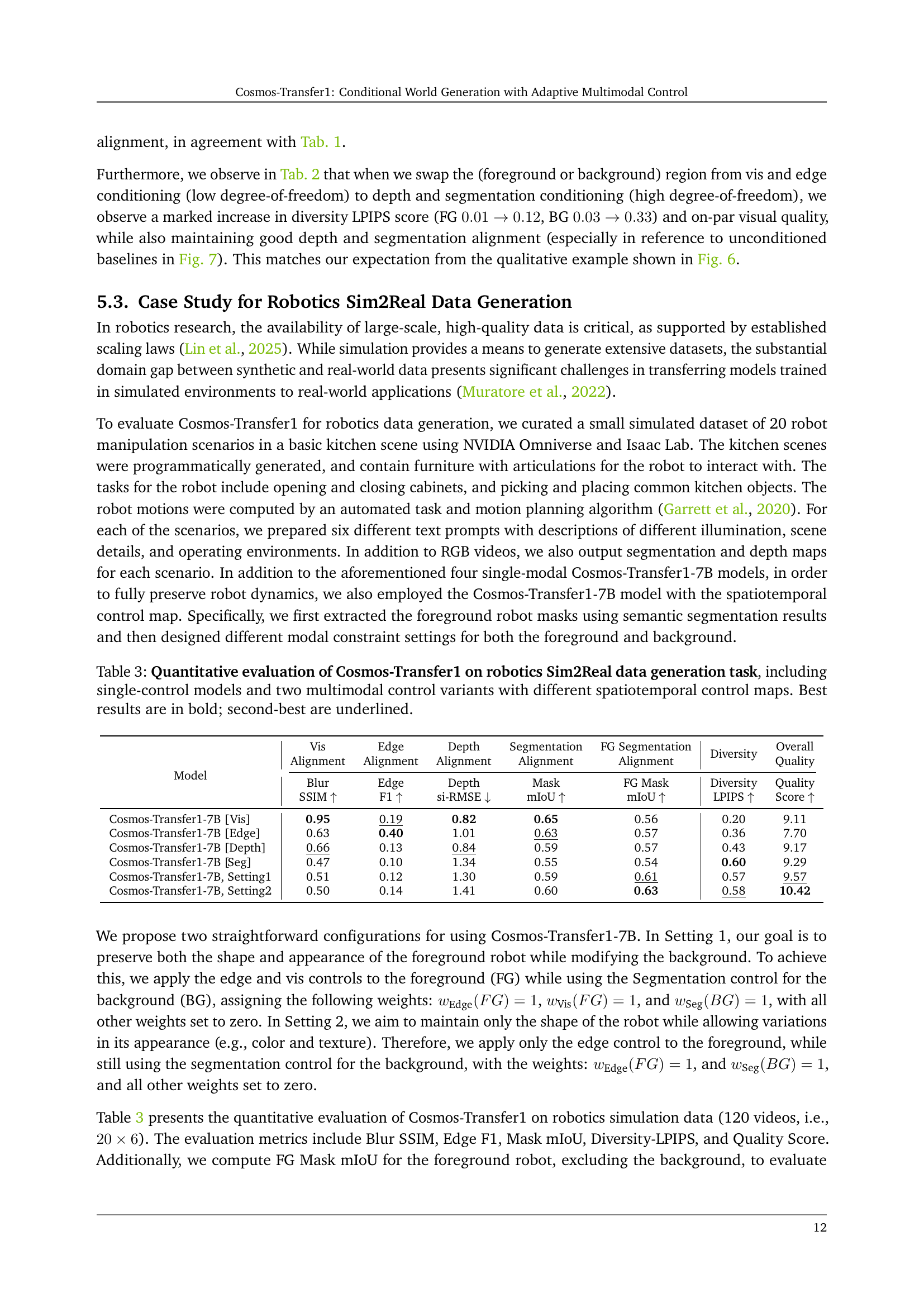
| Model | Vis Alignment | Edge Alignment | Depth Alignment | Segmentation Alignment | FG Segmentation Alignment | Diversity | Overall Quality |
| Blur SSIM | Edge F1 | Depth si-RMSE | Mask mIoU | FG Mask mIoU | Diversity LPIPS | Quality Score | |
| Cosmos-Transfer1-7B [Vis] | 0.95 | 0.19 | 0.82 | 0.65 | 0.56 | 0.20 | 9.11 |
| Cosmos-Transfer1-7B [Edge] | 0.63 | 0.40 | 1.01 | 0.63 | 0.57 | 0.36 | 7.70 |
| Cosmos-Transfer1-7B [Depth] | 0.66 | 0.13 | 0.84 | 0.59 | 0.57 | 0.43 | 9.17 |
| Cosmos-Transfer1-7B [Seg] | 0.47 | 0.10 | 1.34 | 0.55 | 0.54 | 0.60 | 9.29 |
| Cosmos-Transfer1-7B, Setting1 | 0.51 | 0.12 | 1.30 | 0.59 | 0.61 | 0.57 | 9.57 |
| Cosmos-Transfer1-7B, Setting2 | 0.50 | 0.14 | 1.41 | 0.60 | 0.63 | 0.58 | 10.42 |
🔼 This table presents a quantitative comparison of different Cosmos-Transfer1 model variations on a Sim2Real robotics data generation task. It assesses the performance of single-modality control models (using only one input type like visual, edge, depth, or segmentation) against two multimodal control models that leverage combinations of these inputs. The multimodal models use distinct spatiotemporal control maps to differentially weight the input modalities. The table evaluates performance using metrics such as Blur SSIM, Edge F1, Depth si-RMSE, Mask mIoU, and Diversity LPIPS, as well as an overall Quality score. Best and second-best results are highlighted for easier interpretation. The purpose is to demonstrate the impact of using multiple modalities and adaptive weighting schemes for improved realism and control in generating simulated robotics data.
read the caption
Table 3: Quantitative evaluation of Cosmos-Transfer1 on robotics Sim2Real data generation task, including single-control models and two multimodal control variants with different spatiotemporal control maps. Best results are in bold; second-best are underlined.
| Method | 3D-Bbox mAP | Lane mIoU | Reprojection Err. |
| Cosmos-Transfer1-7B-Sample-AV [HDMap] | 41.89 | 50.37 | 9.46 |
| Cosmos-Transfer1-7B-Sample-AV [LiDAR] | 46.50 | 48.19 | 8.60 |
| Cosmos-Transfer1-7B-Sample-AV | 44.66 | 51.55 | 8.67 |
🔼 Table 4 presents a quantitative comparison of the Cosmos-Transfer1-7B-Sample-AV model’s performance on autonomous driving video generation. It evaluates three different model configurations: using only HDMap as a control signal, using only LiDAR as a control signal, and using both HDMap and LiDAR as combined control signals. The evaluation metrics include 3D bounding box mean Average Precision (mAP), lane mean Intersection over Union (mIoU), and photometric reprojection error. This allows assessing how well the generated videos align with the control signals and the overall quality of the generated data for autonomous driving applications. The best results for each metric across all model configurations are highlighted in bold.
read the caption
Table 4: Quantitative evaluation of Cosmos-Transfer1-7B-Sample-AV on the autonomous driving video generation task. We compare the results of both single-control models and multimodal control variant over various metrics. Best results are in bold.
| Number of GPUs | 1 | 4 | 8 | 16 | 32 | 64 |
| Diffusion only | 141.0 s | 39.3 s | 20.1 s | 10.3 s | 5.4 s | 3.5 s |
| End-to-end | 141.7 s | 40.0 s | 20.8 s | 11.0 s | 6.1 s | 4.2 s |
🔼 This table presents the computation time required to generate a 5-second video using the Cosmos-Transfer1-7B model under various levels of parallelism. It demonstrates the significant speedup achievable by increasing the number of GPUs used for processing. The results highlight the scalability of the model and its ability to achieve real-time generation speeds when utilizing a sufficient number of GPUs (specifically, 64 B200 GPUs). The table compares the diffusion-only computation time against the end-to-end runtime (including all aspects of video generation).
read the caption
Table 5: Computation time for generating a 5-second video with Cosmos-Transfer1-7B under different parallelism settings. End-to-end runtime dips below 5 seconds when scaled up to 64 B200 GPUs and reach real-time generation throughput.
Full paper#
